Performance of Turbulence Models in Simulating Wind Loads on Photovoltaics Modules

Abstract

The performance of five conventional turbulence models, commonly used in the wind industry, are examined in predicting the complex wake of an infinite span thin normal flat plate with large pressure gradients at Reynolds number of 1200. This body represents a large array of Photovoltaics modules, where two edges of the plate dominate the flow. This study provided a benchmark for capabilities of conventional turbulence models that are commonly used for wind forecasting in the wind energy industry. The results obtained from Reynolds Averaged Navier-Stokes (RANS) $k-\epsilon$, Reynolds Normalization Group (RNG) $k-\epsilon$, RANS $k-\omega$ Shear Stress Transport (SST) and Reynolds Stress Model (RSM) were compared with existing Direct Numerical Simulations (DNS). The mean flow features and unsteady wake characteristics were used as testing criteria amongst these models. All turbulence models over-predicted the mean recirculation length and under-predicted the mean drag coefficient. The major differences between numerical results in predicting the mean recirculation length, mean drag and velocity gradients, leading to deficits in turbulence kinetic energy production and diffusion, hint at major difficulties in modeling velocity gradients and thus turbulence energy transport terms, by traditional turbulence models. Unsteadiness of flow physics and nature of eddy viscosity approximations are potential reasons. This hints at the deficiencies of these models to predict complex flows with large pressure gradients, which are commonly observed in wind and solar farms. The under-prediction of wind loads on PV modules and over-estimation of the recirculation length behind them significantly affects the efficiency and operational feasibility of solar energy systems.

1. Introduction

The flow structures formed behind bluff bodies generate a recirculating flow region that is referred to as the “wake”. This phenomenon has been extensively examined both numerically [1,2,3,4,5] and experimentally [6,7,8]. Flat plates are one of the simplest geometries that produce a fundamental wake for testing turbulence models and numerical schemes [5]. Moreover, flat plates represent the geometrical shape of Photovoltaic (PV) modules, the market for which is increasingly growing. Accurate simulation of wind flows over PV modules is a key part in optimizing PV systems, especially rooftop-mounted PV modules in urban areas. Wind loads can cause damages to PV panel and thus data monitoring is critical [9]. The complex and multi-directional nature of the wind in such environment makes it difficult to predict the resultant wake behind sharp-edge bluff bodies, such as buildings, PV modules and terrains [10]. Furthermore, correct prediction of wind flow in complex terrains, where large pressure gradients are expected, is crucial in improving the performance of wind farms, safe placement of PV modules due to wind loads and modeling the wake of buildings in urban communities. For example, accurate prediction of wind loads on PV modules is especially relevant at high latitudes where solar panels need to be rather tilted in order to work efficiently. The high angle between the panels and the rooftops results in large aerodynamic forces on solar panels, which in turn causes a structural safety issue that require strengthening of the roof. In these situations, the installation cost of the system can get as high as ≈50% of the PV system [11]. Therefore, the implications of using an appropriate means for predicting wind loads and wind flow forecasting in general, is enormous in the renewable energy industry. Moreover, accurate prediction of the wake formed behind PV modules and wind loads on large arrays play a crucial role in architecture of solar farms and large-scale solar energy system implementation in urban communities. Here, we focus on using the wake of a flat plate as a simple and fundamental flow to examine the performance of five turbulence models in predicting critical wake features. Thus, we provide a benchmark on the accuracy and applicability of these models in predicting the flow in complex settings and large pressure gradient environment.

The wind loads on PV modules can be estimated by numerical simulations based on Direct Numerical Simulations (DNS) [2,12,13], LES [5,14,15] and Reynolds Averaged Navier-Stokes (RANS) [16,17,18,19,20], or by experiments [8,21,22,23]. PV modules are often represented by thin flat plates, with a certain value of aspect ratio ($AR$) defined as the ratio of the plate height to width. The studies on the wake of thin flat plates have mainly focused on analyzing the changes in the flow topology and wake structures and flow characteristics such as recirculation length, drag and vortex shedding frequency. Most experimental studies are restricted to high Reynolds numbers of $Re=U_{\infty }h/\nu ={10}^4-{10}^5$, where $U_{\infty }$ is the freestream velocity, h is the plate height and $\nu$ is the fluid viscosity. DNS studies are mostly limited to low $Re$s ($\le 3\times {10}^3$) due to the extensive computational costs at higher $Re$. Numerical studies based on LES, however, enable increasing the $Re$ to moderate to high ranges (${10}^3-1.5\times {10}^5$). Moreover, studies using RANS models extend the range of $Re$ by modeling complex features of the flow instead of solving for them as in the case of LES and DNS [19]. Despite the simple geometry of a flat plate, when it comes to comparing numerical and experimental results, the literature highlights crucial discrepancies in predicting accurately the wake properties. This lack of agreement amongst experimental and numerical studies has been attributed to wind tunnel scaling issues for the former [24] or strong $Re$ effects, boundary conditions, turbulence modeling and computational domain size for the latter [5]. Therefore, it is important to have a benchmark on how different numerical tools, that is, turbulence models, perform in predicting such complex flows despite the simple geometry of a sharp-edge flat plate.

The studies of wind loading on PV modules can be classified into two categories: roof-mounted and ground-mounted PV panels. Both categories can be subjected to wind-related structural failures, especially when the system experiences multi-directional and turbulent wind flow during extreme wind events. Beside the influence of incident wind angles of attack, the tilt angles of PV panels can also affect the lift and drag forces (pressure distributions) under wind loading on the panels surface. These studies included numerical [17,18,19,20] and experimental [21,22,25,26] investigations of the wind load based on the flow around PV panels for different angles of attack ($0^{\circ }$ to ${180}^{\circ }$) and different tilt angles of PV panels. Based on unsteady RANS simulations of the wind load around a ground-mounted PV module with ${25}^{\circ }$ panel tilt angle and different incident wind directions ($0^{\circ }$ to ${180}^{\circ }$ at ${45}^{\circ }$ increments), Jubayer and Hangan [19] found that the maximum wind loading (drag, lift and overturning moments) were localized near the leading edge of the panel for all incident wind directions. The critical wind directions were $0^{\circ }$ and ${180}^{\circ }$ for the maximum drag and maximum uplift respectively; and ${45}^{\circ }$ and ${135}^{\circ }$ for the maximum overturning moments, which the authors attributed to the asymmetric properties of the flow (wake structures and mean pressure distributions) along the panel centreline. Jubayer and Hangan [19] also compared numerical results with wind tunnel measurements by Abiola-Ogedengbe et al. [22] and reported an agreement within 46%. The experimental results of Abiola-Ogedengbe et al. [22] encompassed the same effects on the wind loading for critical wind angles of attack and the asymmetry of pressure distributions along the wake streamwise centerline for tilt angles of ${45}^{\circ }$ and ${135}^{\circ }$. Furthermore, Abiola-Ogedengbe et al. [22] reported that surface pressure on the PV module surface increased with the panel tilt angles, while Stathopoulos et al. [25] stated that the influence of panel inclination can be significant only for critical incident wind angles of attacks. In addition to study of the influence of wind direction and panel inclination on PV module wind loads, Bitsuamlak et al. [27], Shademan et al. [18] and Warsido et al. [21] also studied the effect of spacing parameters on wind loading and the resulting sheltering effects over an array of solar panels. These studies suggested that the sheltering effect caused by upwind PV panels reduced the wind loads on downwind PV panels when they were arranged in tandem.

The first reliable numerical study of the flow around normal flat plates was by Jahromi et al. [28] based on two-dimensional simulations. Hemmati et al. [29] performed a detailed three-dimensional DNS study to investigate the wake of a normal flat plate for a range of aspect ratios, including the infinite span plate, at $Re$$\ge 1200$. Their study showed that wake characteristics changed for different aspect ratios: $AR=3.2$, representing a typical array of solar panels (scaled); $AR=1.6$ representing a single solar panel; infinite span panel, representing a large array or bounded array of solar collectors. More recently, Hemmati et al. [5] expanded their study by evaluating the source of discrepancy between LES and DNS simulations for this flow. Fifteen simulations with varying grid resolution, computational domain size and boundary conditions were performed to investigate their effect in the wake dynamics and also the differences amongst existing numerical and experimental studies. They validated their DNS results at $Re=1200$ with experimental and numerical studies corresponding to $Re\ge$ 1000. This led to the conclusion that the discrepancies observed in the literature at $Re<$ 1000 regarding flow features such as pressure distribution on the plate leeward face are induced by strong $Re$ effects. Furthermore, it was shown that LES method over-predicted the mean drag coefficient and under-predicted the mean recirculation length. This deviation was related to the inability of LES model to capture negative production of the turbulence kinetic energy (k) in a small region immediately behind the body.

Tian et al. [15] used LES to study flow normal to a flat plate at $Re=10\times {10}^5$. The study included two different cases; one in which the plate had rounded off corners based on the curvature of a radius $r=0.01h$ (where h is the plate height) and the other based on a radius $r=0.005h$. The results showed unsteadiness in the flow pattern, which switched between high and low drag regimes. This switch was more frequent for the case with sharper corners, hence indicating that sharp corners increase the mean drag on the plate and the kinetic energy in the near wake. Another LES study [30] investigated the flow around a flat plate at $Re=750$. Two different flow angles were examined: normal plate and plate inclined at ${45}^{\circ }$. This study concluded that the present methodology could be used in engineering applications to predict the effect of wind gust on the wake of sharp-edge bluff bodies despite differences with existing DNS and experimental results.

The wake of an infinite span thin flat plate is unsteady with a low frequency secondary flow [8,29,31]. The effect of the secondary flow on wake dynamics is complex and leads to three different periods of vortex shedding. During the period of low-drag, labeled as Regime L (for Low Amplitude) by Hemmati et al. [29] and Najjar and Balachandar [31], the recirculation region is elongated due to extension of the shear layer, the vortex shedding is suppressed and drag values decrease. The wake loses its coherence and the vortex roll-up is moved away from the panel. The shorter-periods of higher-drag (Regime H—for High Amplitude—based on References [29,31]), occurs when the extended shear layers collapse and force the structures to move towards the panel. This shortens the recirculation region, enhances the pressure drop and magnifies the drag coefficient. Once the secondary effects are propagated out of the near wake region, the wake returns to its natural state with a moderate drag value (Regime M—for Moderate Amplitude—according to Reference [29]). The complexity of the wake of infinite span flat plates despite its simple geometry makes it an interesting bluff body to investigate, particularly regarding the performance of turbulence models.

RANS models have been used to predict wind loads on solar panels in a number of studies. Particularly, these studies focused on ground-mounted panels [32,33] and rooftop-mounted panels [34]. The comparisons were high-level validation-based analysis with experimental results and they lacked extensive review of the simulation results. For example, Roy et al. [35] compared Detached Eddy Simulation (DES) and RANS models in simulating the wake of a square cylinder at $Re=2.4\times {10}^4$. Their findings suggested that RANS models have major difficulties in capturing the correct mean recirculation length. Moreover, it was identified that RANS models severely under-predicted the turbulence production. Although there is substantial literature on RANS models and their overall behavior for different flows, there are no major studies, to the authors knowledge, that focus on the performance of RANS models in predicting complex wakes with large pressure gradients in comparison to DNS simulations. Such conditions are common in wind forecasting over complex terrains, which is crucial in wind energy industry.

This paper aims at providing detail information on performance of steady and unsteady RANS models in evaluating the wake dynamics of normal thin flat plates with infinite span. The study focuses on determining main wake characteristics, such as mean recirculation length, drag coefficient, pressure distributions and profiles of velocity and stresses for each turbulence model. The results are compared with DNS results of Hemmati et al. [5,29]. This study is to serve as a benchmark in identifying the limitations of conventional steady and unsteady RANS models in accurately predicting the wake of sharp-edge bodies and complex terrains with large pressure gradients. The problem description is presented in Section 2, followed by the results and comparison of the model performances in Section 3. A summary of the main findings are reported in Section 4.

2. Problem Description

This study investigated the performance of different RANS and Unsteady-RANS (URANS) models on predicting the characteristics of a uniform flow around a normal thin flat plate with infinite span. This geometry corresponds to a large array (36 modules) of panels placed normal to the flow. The angle of inclination for the modules was selected as normal to horizontal axis for two reasons: (1) to examine the performance of RANS and URANS models in predicting a complex wake involving secondary flows (low frequency incidents) that lead to large unsteady variations and large pressure-gradients [31] and (2) the most critical design criteria with respect to wind loading and drag. Thus, this platform provides insight into the performance of RANS models in design of infrastructure for PV modules installations.

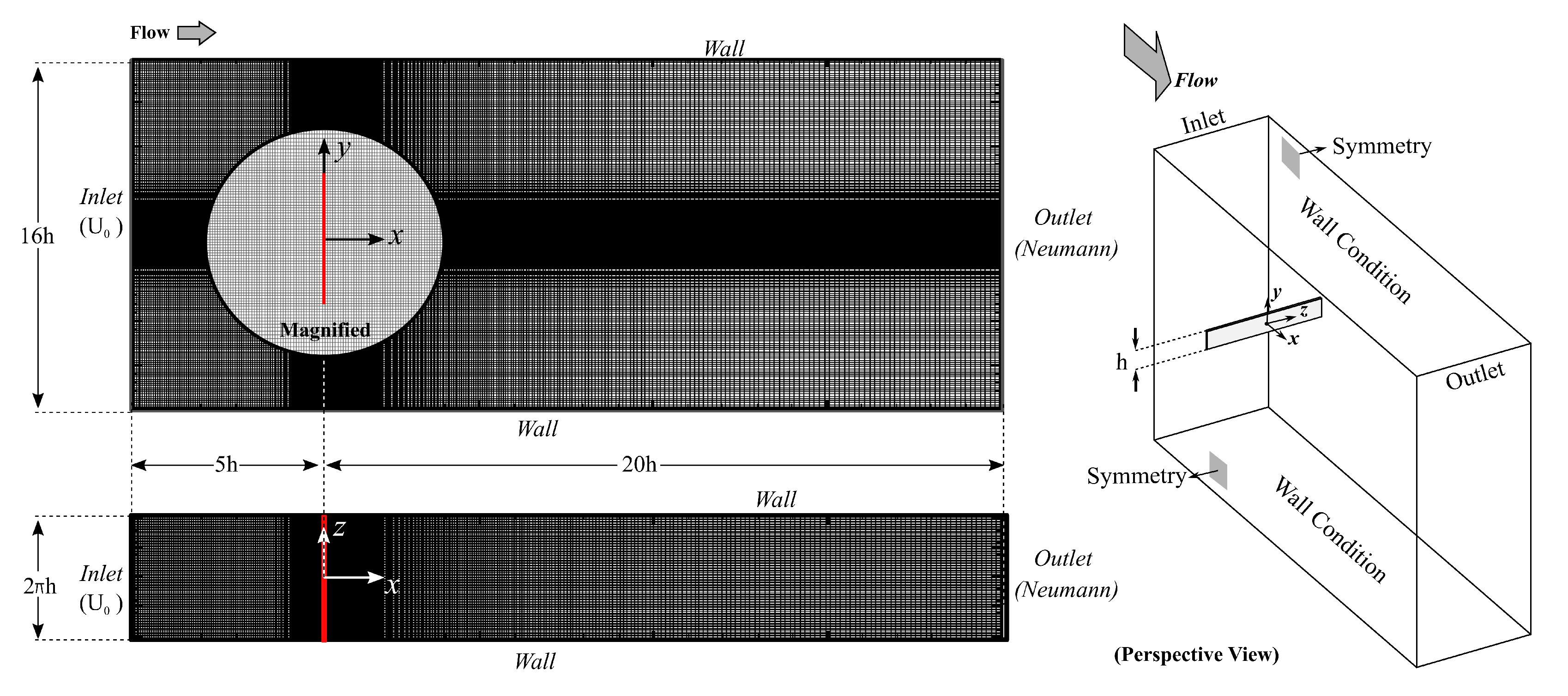
The computational domain for the present simulations is defined in a three-dimensional Cartesian coordinate system, which is shown in Figure 1, with a rigid stationary thin flat plate located at the origin. The x-axis is in the streamwise direction, y-axis in the chordwise direction and z-axis in the spanwise direction. The rigid flat plate has a height of h and its thickness is that of the smallest spatial grid.

The computational domain was designed following Najjar and Balachandar [31] and Hemmati et al. [29], in which the domain extended from $-5h$ to $+25h$ in the streamwise ($x-$) direction with the plate located at the origin, from $-8h$ to $+8h$ in the chordwise ($y-$) direction and $-\pi h$ to $\pi h$ in the spanwise ($z-$) direction. The streamwise distance between the plate and outlet boundary allows for flow re-development (recovery) after the wake region. The inlet boundary is located $5h$ upstream of the plate, which is sufficient to prevent artificial acceleration of the flow [5]. The recommended spanwise size is $2\pi h$, which allows capturing three-dimensional features of the flow [2] and the plate is extended across the entire span of the domain.

An in-homogeneous spatial grid compiled of unstructured hexahedron elements (Figure 1) is used for these simulations. The computational grid is refined in area of interest to accurately capture major wake phenomena such as vortex structures and shear layers that are dominated by large velocity and pressure gradients. Thus, the finest elements are placed around the plate and in the near wake. Furthermore, the plate thickness was that of the smallest element in the x-direction, in order to represent a thin flat plate without any reattachment effects in the flow. The non-uniformity of the grid followed strict guidelines to avoid large element skewness and grid quality issues. Moreover, the grid quality was ensured to be sufficiently high by checking main grid parameters such as orthogonal angle, expansion factor and aspect ratio. For the unsteady case, the temporal grid was set such that the maximum Courant number (CFL) does not exceed 0.48.

The RANS and URANS equations [36] are computed using five different turbulence models—(SIM-1) Standard $k-\epsilon$, (SIM-2) SST $k-\omega$, (SIM-3) RNG $k-\epsilon$, (SIM-4) BSL RSM and (SIM-5) Unsteady $k-\epsilon$. The details of the turbulence modeling formulations for the aforementioned models can be found in References [37,38,39,40]. The discretization of Navier Stokes equations is based on a finite-volume approach. ANSYS CFX was used as the main solver. High resolution schemes, which are second-order accurate and bounded are used for advection fluxes, viscous terms and turbulence numerics. The convergence criteria for the simulations was defined by the residual momentum root mean square value, which was set to ${10}^{-6}$. The simulations were completed using 6 CPUs and 64 GB of memory.

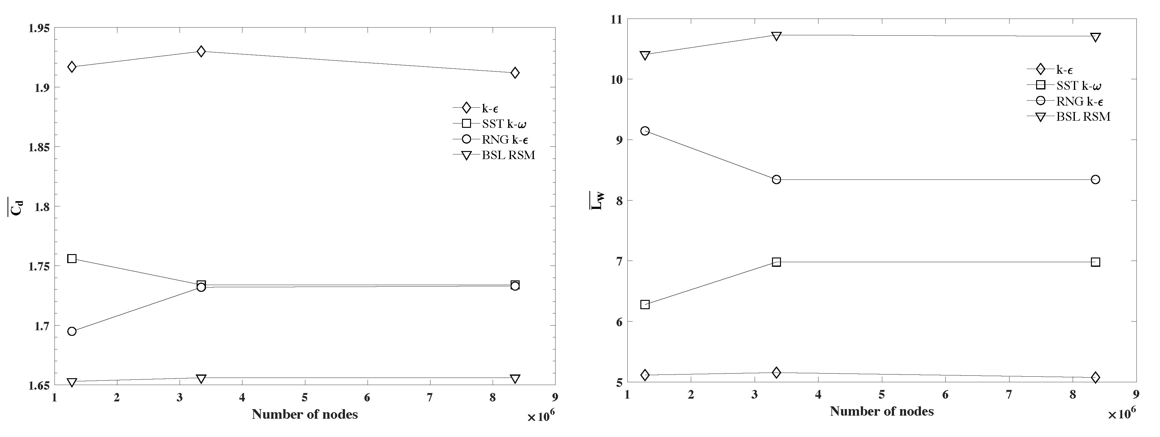
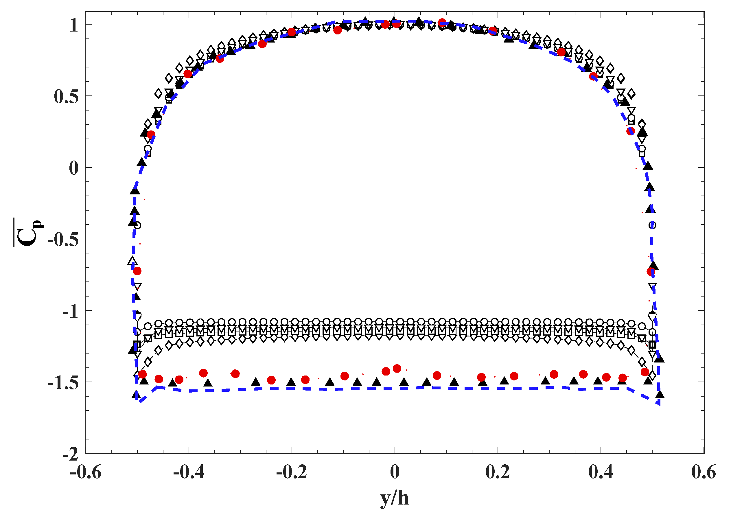
Grid Independence Analysis

A quantitative grid independence analysis from twelve simulations was completed to confirm the results are grid-independent. Three different grids with the same in-homogeneous grid distribution and quality were designed for this analysis: Grid 1 with $1.27\times {10}^6$ elements, Grid 2 with $3.34\times {10}^6$ elements and Grid 3 with $8.36\times {10}^6$ elements. The mesh-sensitivity study was based on two parameters, the mean drag coefficient ($\overline{C_d}$) that is mainly dominated by the pressure differences and the mean recirculation length ($\overline{L_w}$). The results from the mesh independence analysis for each turbulence model are displayed in Figure 2.

The differences of both $\overline{C_d}$ and $\overline{L_w}$ obtained by the finest grids was less than $1\%$, which allowed us to consider the intermediate grid (Grid 2) as the appropriate grid for the simulations. Since we use the same grid distribution as that of Hemmati et al. [5] and based on an their extensive grid and boundary condition sensitivity analysis, the observed differences of ≤1% constitutes grid-independence for these simulations.

3. Results & Discussion

The performance of four steady models are first examined in terms of their prediction of global flow variables, wake profiles and streamlines. This is followed by examining the performance of unsteady RANS models in comparison to DNS results and those of steady models.

3.1. Steady RANS Models

We begin by examining the time-averaged (mean) wake topology computed by four turbulence models. First, we consider the streamlines depicted in Figure 3, which shows the overall structure of the flow field. All models succeeded in predicting the overall features of the mean wake, such as flow separation and shear layer roll-up at the edges, leading to the formation of a large recirculation region in the near wake of the plate. The mean streamlines were symmetric to the wake centreline and exhibited two parallel vortices rotating in the opposite direction. This is comparable to the mean wake shown by Hemmati et al. [5]. However, the recirculation region is over predicted in length and in width by all models, although SIM-4 (RSM model) provides the most deviation from the DNS results. The enlarged recirculation region coincides with an over-prediction of the angle of separation at the plate edges. Previously, Hemmati et al. [5] showed that the mean recirculation length is over-predicted by Large-Eddy-Simulations, which they attributed to the limitations imposed by the implementation of Eddy Viscosity and Boussinesq approximations. A similar behavior in predicting the mean streamlines are also seen here for all the simulations, which are based on similar implementations of Eddy Viscosity and Boussinesq approximations.

A quantitative analysis of main wake properties, such as the mean recirculation length, mean drag coefficient and profiles of mean surface pressure coefficients, showed significant differences compared to the reference DNS.

Table 1. Comparing the mean drag coefficient and recirculation length for different turbulence model, with the Direct Numerical Simulation (DNS) results at similar Reynolds number ($Re=1200$).

Case	Method	$\overline{{\mathit{C}}_{\mathit{d}}}$	$\overline{{\mathit{L}}_{\mathit{w}}}/\mathit{h}$
SIM-1	Standard k-$\epsilon$	1.93	5.15
SIM-2	SST k-$\omega$	1.73	6.98
SIM-3	RNG k-$\epsilon$	1.73	8.34
SIM-4	BSL RSM	1.66	10.73
Hemmati et al. [5]	DNS	2.13	2.65

compares global (integral) flow variables amongst the four turbulence models. One noticeable difference is on the prediction of mean drag coefficient. All models under-predicted the mean drag coefficient, with SIM-4 giving the least accurate prediction and SIM-1 giving the closest value compared to DNS. The SST k-$\omega$ model in SIM-2 was second, followed by the RNG k-$\epsilon$ model in SIM-3.

As observed previously from the streamline plots in Figure 3, neither of the RANS models accurately predicted correct extent of the recirculation zone in the near wake (see Table 1). The mean recirculation length was largely overestimated by all models, with SIM-4 giving the highest overestimation. Amongst these models, the RSM model (SIM-4) gave the largest difference compared to DNS, while the standard k-$\epsilon$ model (SIM-1) performed better, even though there were significant differences with DNS results. This lack of accuracy is also related to the differences observed in prediction of pressure. There is, intuitively, a correlation between correct prediction of the mean recirculation length, mean drag and mean surface pressure, which are sensitive to the predicted location of the recirculation vortex centres based on the relation identified in source terms of the Poisson equation (for more details see Hemmati et al. [41]). Thus, this relates to the correct prediction of the velocity and pressure gradients in the wake.

Amongst the models themselves, the predictions of windward surface pressure on the plate (Figure 4) are similar, where smaller gradients are expected. The minor differences observed in comparison to DNS results evidently contribute to the under-prediction of mean drag and it can be attributed to inaccurate prediction of the angle of separation at sharp-edges of the plate leading to inaccurate prediction of gradients in the shear layer. The major deviation, however, appeared in the base pressure, on the leeward face of the plate, which is responsible for the extreme under-prediction of mean drag. This can also be identified as an indicator that the back surface pressure distributions are highly sensitive to complex and unsteady changes in the wake topology.

The profiles of turbulence kinetic energy and mean velocity are compared amongst the models along the wake centreline in Figure 5. The mean streamwise velocity ($\overline{u}$) showed similar trend along the wake centreline (Figure 5), which included overestimation of the mean recirculation length. The stagnation point was located closed to the plate for DNS, which resulted in a shorter recirculation length. SIM-4 provided the largest deviation from the DNS and SIM-1 the closest flow prediction to the DNS. Furthermore, the wake predicted by SIM-1 exhibited a larger velocity deficit in the recirculation region behind the plate compared to other RANS models. This was consistent with the observations of Roy et al. [35] for square cylinders. The turbulence kinetic energy ($k=0.5(\overline{u^{\prime 2}}+\overline{v^{\prime 2}}+\overline{w^{\prime 2}})$ where $u^{\prime }$, $v^{\prime }$ and $w^{\prime }$ are random components of velocity) was larger in stagnation region in close proximity of the plate in SIM-1, even though k remained far lower than those observed from DNS (Figure 5). In fact, the DNS study predicted the magnitude of turbulent kinetic energy in the vortex zone more than three times that of the steady RANS models. The wake velocity deficits from the eddy viscosity models resulted in elongated recirculation distances, smaller mean velocity and lower turbulent kinetic energy, where peak values reached farther into the wake compared to DNS.

The simulations presented so far are based on steady RANS models that do not properly capture the flow unsteadiness by the virtue of their formulations. Since they also fall short in accurately predicting the mean wake, it can be argued that the unresolved flow unsteadiness significantly impacts the mean flow field. This is specially true for the wake of a normal infinite span thin flat plate, which is identified as extensively complex with underlying secondary (low-frequency) features [8,29,31]. Thus, the significant unsteadiness of the wake of sharp-edge bluff bodies with large pressure gradients, such as flat plates, require an unsteady model to correctly predict both the mean and instantaneous flow fields. This hypothesis is examined by modeling the wake using Unsteady-RANS k$-\epsilon$ model (SIM-5) and comparing it with steady RANS k$-\epsilon$ model (SIM-1) and DNS.

3.2. Unsteady RANS Model

The unsteady RANS analysis in SIM-5 was carried out using Grid 2 (Figure 1) based on the unsteady $k-\epsilon$ model. The total simulation time was correlated with the statistical convergence in the turbulent field. Thus, statistical convergence was reached after 50 vortex shedding cycles.

Figure 6 shows the streamline plot of the wake central $xy-$plane from SIM-5. Slight improvements in predicting the mean recirculation distance was observed in comparison to the previous streamline plots for SIM-1 in Figure 3a. For example, the vortex cores were closer to the plate and the stagnation region was specified within a shorter distance ($\overline{L_w}=4.47h$), compared to the previous mean recirculation length of $5.15h$. Moreover, the shorter mean recirculation region coincided with higher vorticity of the detached structures, which led to an augmentation of mean drag by almost 9% (for SIM-5, $\overline{C_d}=2.1$). Since wake structures are closer to the plate, the viscous forces acting on the plate are magnified due to their correlation with larger velocity gradients caused by the higher vorticity structures. Thus, the unsteady $k-\epsilon$ model computed a relatively larger $\overline{C_d}$. The value of the mean drag coefficient calculated by the unsteady $k-\epsilon$ agrees well with the result reported in the literature [5,12,32]. Thus, the unsteady $k-\epsilon$ model has relatively succeeded in predicting the mean drag by allowing unsteady behavior of the flow. However, there were still large differences with respect to prediction of the turbulence field in close proximity of the plate. The reported recirculation region remains largely overestimated in length and width compared to existing results in literature. This suggests that the previously hypothesized effect of unsteady flow on mean wake prediction with respect to the estimation of mean recirculation length may be partially valid with the correct prediction of the mean drag only. The limitations of steady RANS models in accurately predicting the unsteady wake of a flat plate is further analyzed by comparing the wake features for steady and unsteady RANS models and the DNS.

The profiles of mean streamwise velocity ($\overline{u}$) are compared in Figure 7. Although SIM-5 predicted a shorter recirculation length and the overall trend agrees with the DNS but velocity substantially increases rather quickly to that of the freestream. The velocity deficit remains smaller than the DNS but similar to SIM-1. The turbulent kinetic energy along the centerline is also shown in Figure 7. The results from SIM-5 tends to behave similar to the DNS. However, turbulence kinetic energy remains underestimated compared to the DNS. The dislocation of the maximum k follows the overestimation of the mean recirculation length.

The differences in the wake features were further analyzed by examining the profiles of mean velocities and wake turbulence characteristics at $x=5h$ and $x=8h$ in Figure 8 and Figure 9. As observed in previous sections, neither the steady nor unsteady RANS models had accurately predicted the near wake features compared to DNS. The mean streamwise velocity outside the base vortex region ($x=8h$) was overestimated by SIM-5 and significantly under-predicted by steady simulations of SIM-1. At $x=5h$, which is outside the recirculation area for SIM-5, both models largely underestimated the mean streamwise velocity deficits, while SIM-1 computed the nearest prediction for the chordwise velocity compared to DNS.

Distributions of turbulent kinetic energy at $x=5h$ and $x=8h$ are compared in Figure 10. The profiles exhibited major differences in the predictions obtained by DNS compared to SIM-1 and SIM-5. The values of k from DNS was higher in magnitude than those calculated by Steady and Unsteady RANS models. However, it should be emphasized that these large deviations in prediction of turbulence were expected since the mean recirculation length ($\overline{L_w}$) was severely overestimated by both RANS models. These large differences also appeared in the profiles of chordwise Reynolds normal stress (Figure 11). The maximum value of $\overline{v^{\prime 2}}$ was severely underestimate by both SIM-1 and SIM-5, while the profile of these values did not compared well with those obtained by DNS. This further confirms the limitations of RANS models in accurately predicting the unsteady characteristics of the wake, which consequently affects the mean flow field results.

The turbulence dissipation ($\epsilon$) and production ($P_k$) along the wake centreline are compared between SIM-5, SIM-1 and the DNS in Figure 12. Since the models predict different mean recirculation sizes, we have normalized x with the mean recirculation length ($\overline{L_w}$) for each case. Moreover, the production results from DNS are scaled by ${10}^3$ to enable a proper comparison. There are several interesting observations that attribute to the differences observed amongst these simulations. First, the computed turbulence production is significantly smaller for SIM-1 and SIM-5 compared to DNS by four orders of magnitude at its peak. This is consistent with the findings of Roy et al. [35], which showed under-predicted turbulence production by RANS models in the wake of a square cylinder. Second, the eddy viscosity models in SIM-1 and SIM-5 allow for negative production values, which was not the case for LES simulations of Hemmati et al. [5]. However, this did not address the difficulties of these models in accurately simulating the wake. Third, the general behavior of $P_k$ is different for SIM-1 and SIM-5 compared to DNS. The peak at SIM-1 appears prior to the stagnation point, whereas SIM-5 and DNS observe the peak downstream of the stagnation point. However, the peak at SIM-5 is moved farther downstream the stagnation point by ≈0.2$\overline{L_w}$ compared to DNS. In contrast to the production term, the dissipation of turbulence was not substantially underestimated by SIM-1 and SIM-5. The maximum dissipation in the vicinity of the plate was higher in magnitude for the steady case, even though it remained lower compared to DNS. Farther downstream the plate, SIM-5 had the closest prediction of the dissipation rate compared to DNS. The relatively similar values of dissipation despite severe differences in production term hints at major differences in turbulence diffusion, based on variations observed in the flow field. This implies that the wake in SIM-1 and SIM-5 is highly dissipative and thus, the velocity gradients are likely suppressed.

The distribution of steamwise velocity gradient along the wake centerline is compared for the three cases in Figure 13. The velocity gradients for SIM-1 and SIM-5 were suppressed in the vicinity of the plate, where pressure gradients are also largest. However, SIM-5 appears to recover outside of the recirculation region, where pressure gradients are smaller. This explains that the differences observed in the eddy viscosity models of SIM-1 and SIM-5 are almost exclusively due to the inaccurate prediction of the velocity gradients in the near wake region. This was also observed as a potential cause of differences in LES and DNS results by Hemmat et al. [5].

The results have shown that neither the steady nor unsteady conventional RANS models can accurately capture the unsteady wake of an infinite span thin flat plate compared to DNS. The possible explanations for the observed limitations may be attributed to the computational grid or the complexity of three-dimensional wake features. However, since all the simulations in this study used the same optimized grid as well as the reference DNS study, which allowed a fair comparison between results, this possibility was not likely the source of deviations. Despite its simple geometry, the instantaneous wake of an infinite span flat plate is dominated by low frequency secondary features that induce three different periods of vortex shading [29]. Previous studies [8,29,31] have revealed that the presence of secondary instabilities in the vortex shedding significantly enhances the vortex generation and detachment length, leading to major changes in the wake topology and vortex dynamics. Thus, the results so far provide evidence that steady and unsteady RANS models do not accurately capture these secondary features of the flow and this consequently affected the mean flow field results.

4. Conclusions

The performance of steady and unsteady RANS models was studied in simulating the near wake of an array of PV modules, represented by normal thin flat plate with infinite span. The results obtained from the RANS models, which are based on eddy viscosity approximation, were compared to a companion DNS [29].

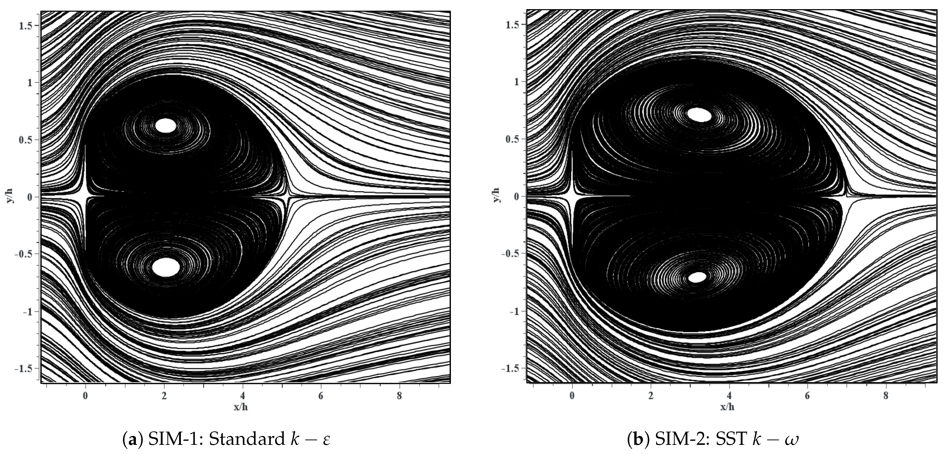
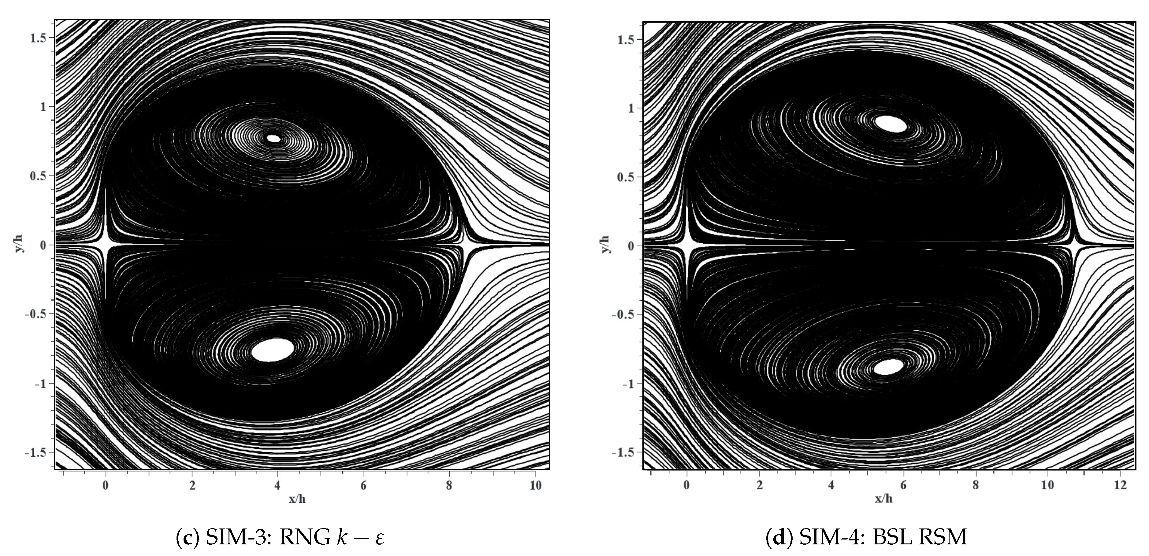
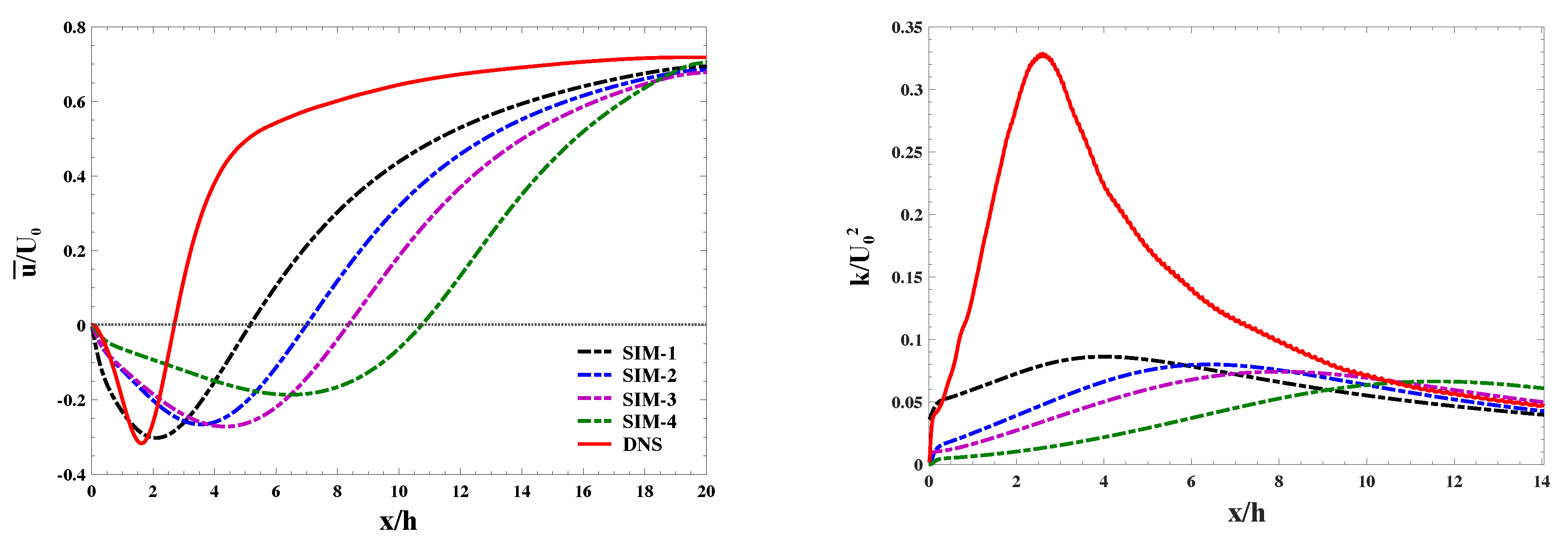
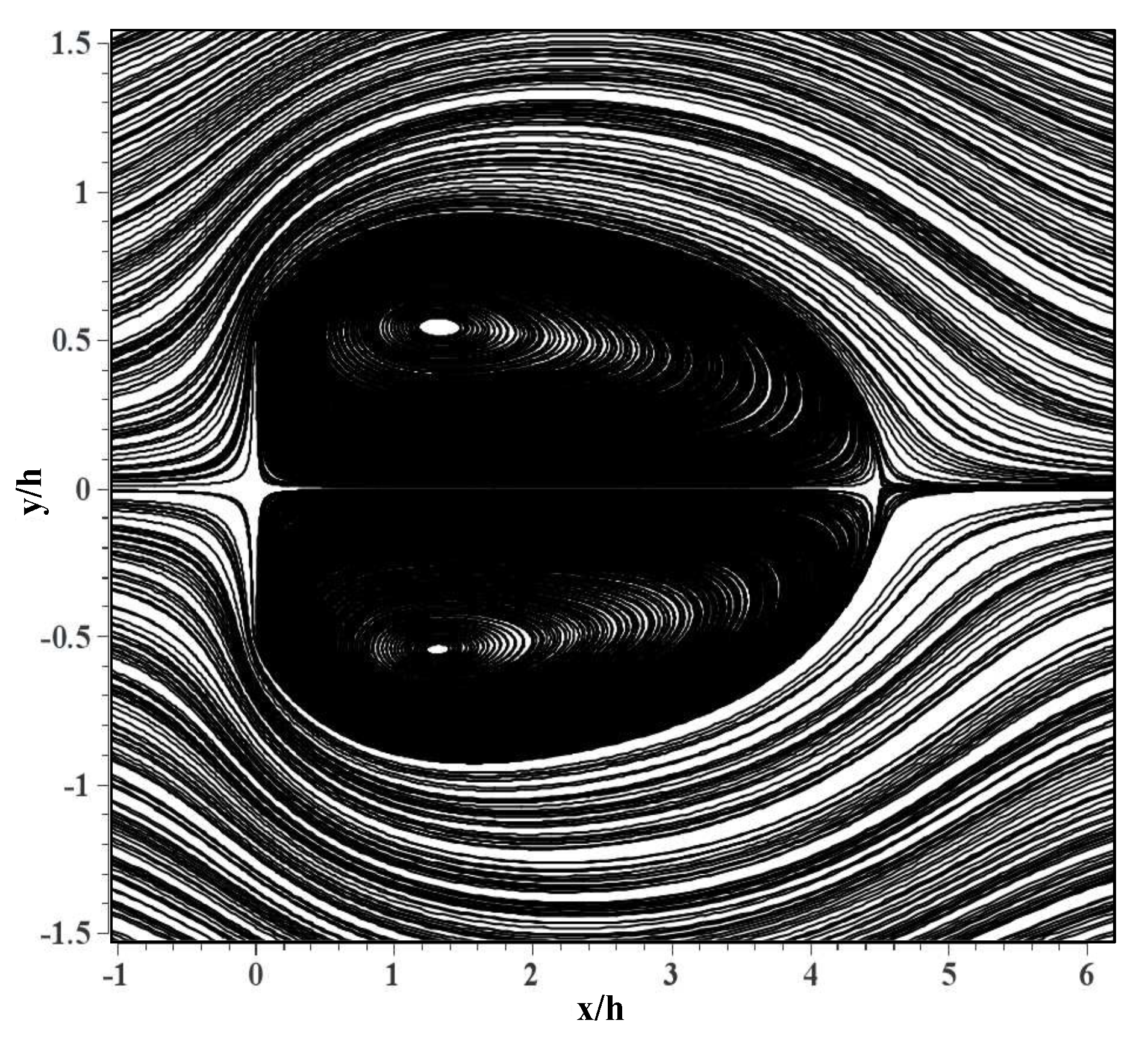
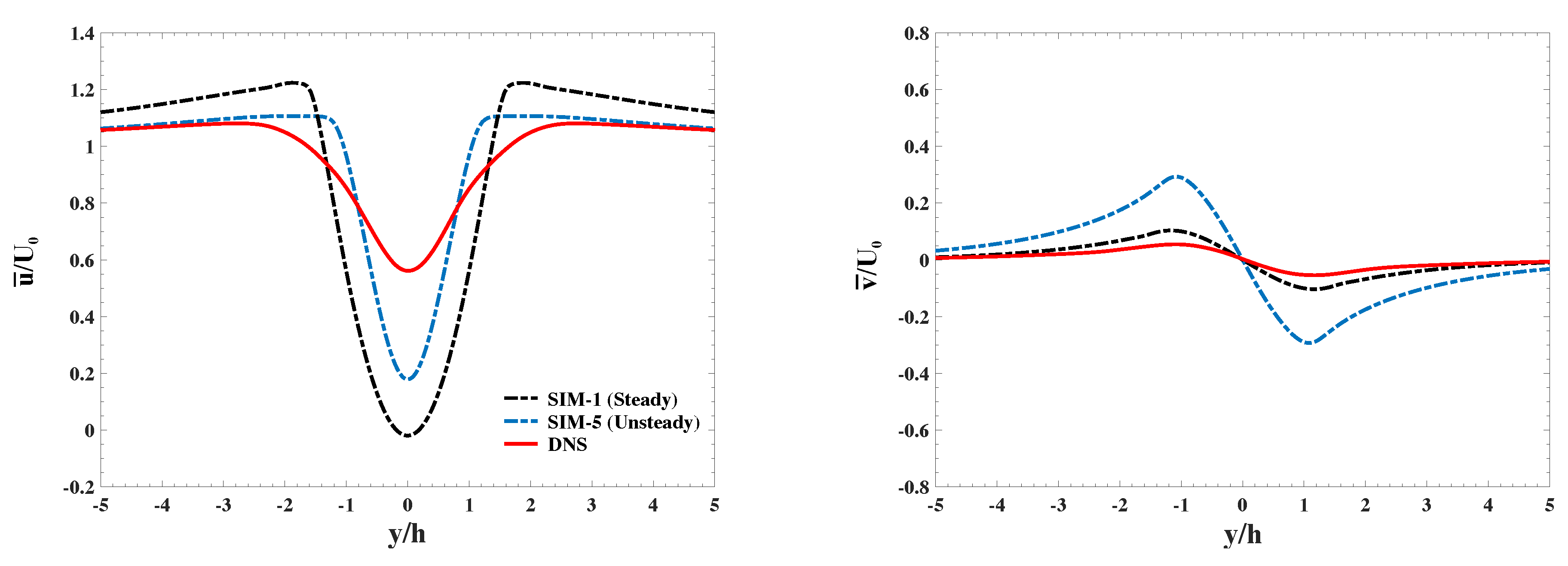
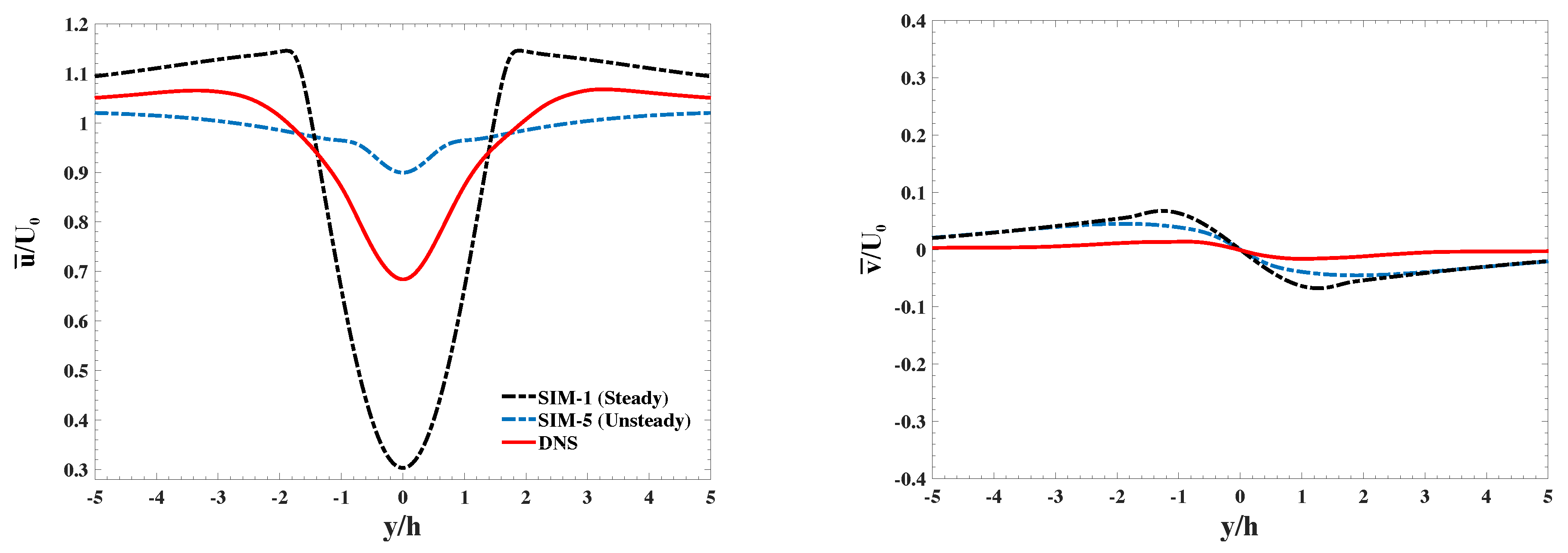
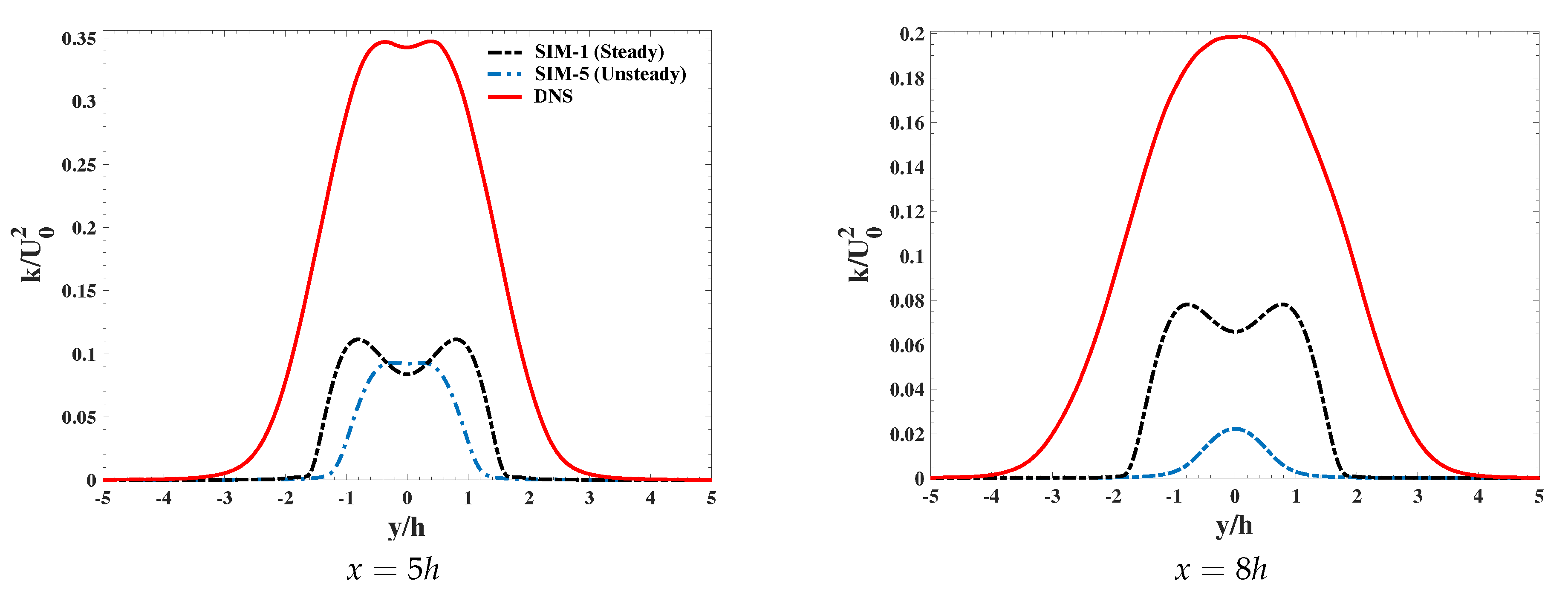
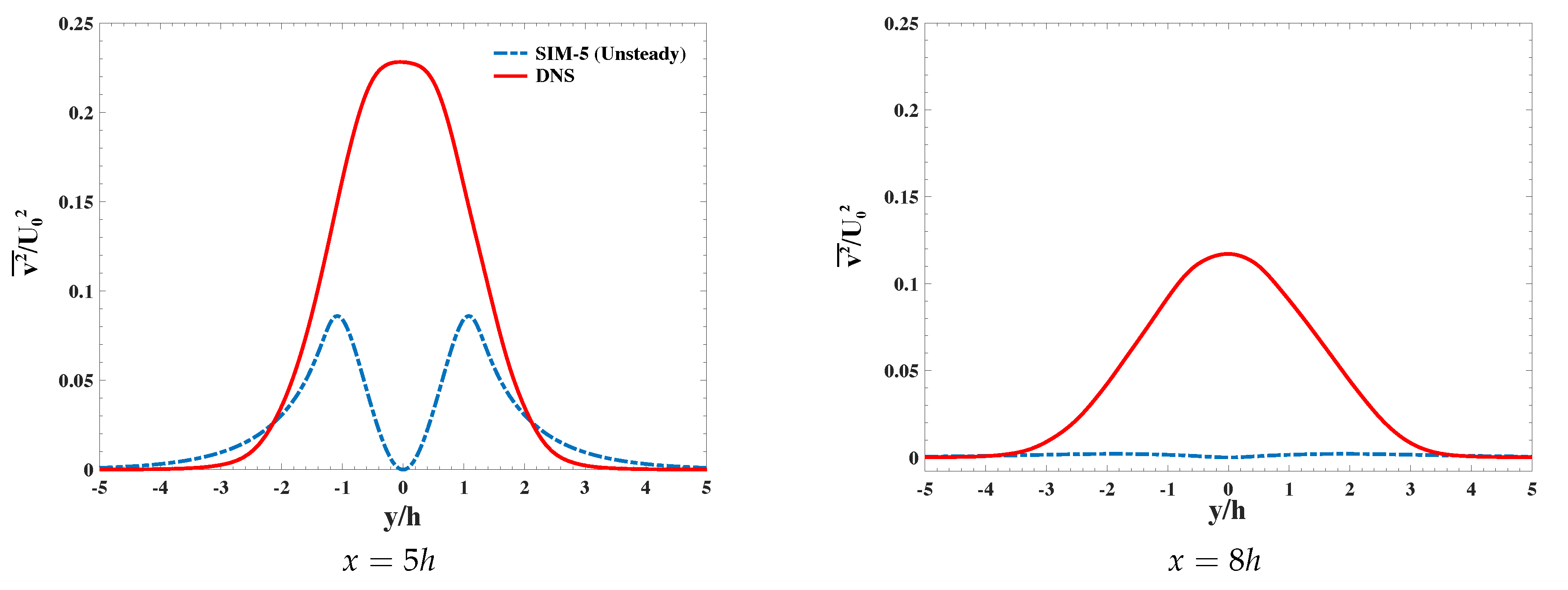
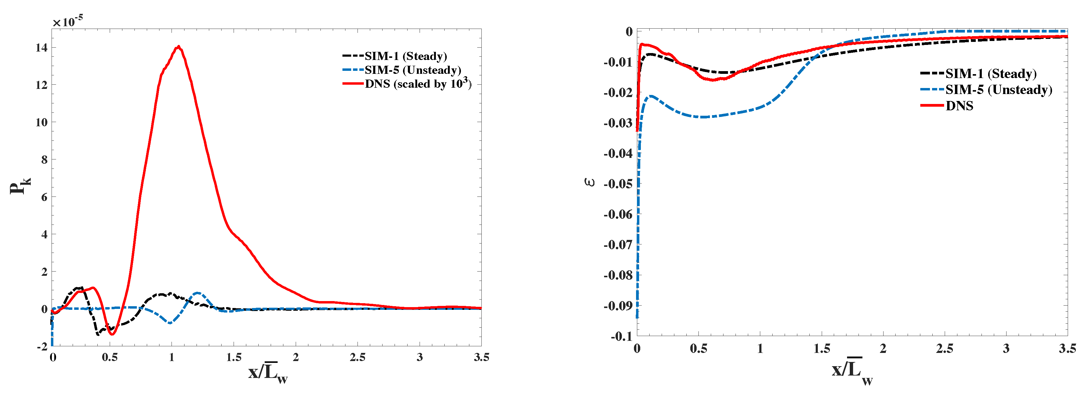
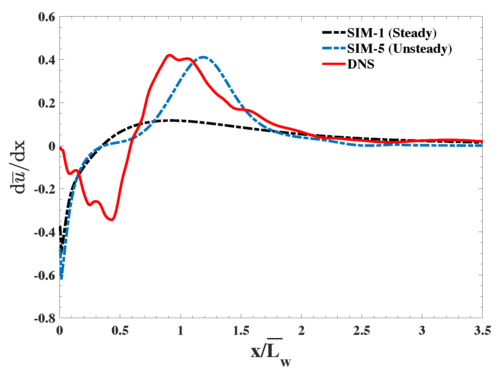
The results from steady RANS models revealed the challenges of different models in predicting the wake feature of an infinite span thin flat plate. Comparing the results with DNS, the similarity appeared in the prediction of global features of the mean flow with a symmetric recirculatory region. However, the shear layer roll up at the edges (flow streamline angles) and the recirculation length were not accurately modeled compared to DNS. Amongst the models tested here, RNG $k-\epsilon$ model performed the worst in predicting mean wake features, whereas the Standard $k-\epsilon$ model provided the closest results to DNS. Thus, this study provided benchmark results indicating the limitations and inaccuracies of steady RANS models in predicting mean flow features due to large pressure gradients, similar to those of complex terrains in wind forecasting. These difficulties were partly attributed to the underlying linear Eddy Viscosity approximation in these models and partly to unsteady nature of the vortex shedding process.

The initial hypothesis that properly capturing the unsteady features of the wake assists in accurate modeling of the flow was also tested using Unsteady RANS $k-\epsilon$ model. Even though improvements were identified in the prediction of mean drag (${\overline{C}}_D=2.1$ compared to 2.13 from DNS), the reported mean recirculation length was overestimated in length and width compared to DNS. However, the results were significantly improved compared to the steady RANS model predictions. Moreover, the turbulence kinetic energy, which was higher than the one predicted by the steady case, remained lower than that of the DNS. Thus, the initial hypothesis was only partially confirmed with more accurate prediction of mean drag, which is attributed to accurate modeling of the pressure field, significant improvements in predicting the mean recirculation length and the wake velocity field. However, there are still significant deviations from DNS results that may hint at the limitations of linear eddy viscosity approximation in modeling complex wakes with major unsteady features. The production of turbulence was severely underestimated by all models, compared to the DNS, while the dissipation was relatively similar. The deficiencies of traditional RANS models in accurate estimation of velocity gradients in the wake of infinite span flat plates are attributed to the limitations of linear eddy viscosity approximation and the steady-based nature of RANS formulations in modeling the highly unsteady vortex shedding process behind flat plates.

These results illustrate that conventional RANS models are not sufficiently accurate in predicting the wind loads on arrays of PV modules. Moreover, they fall short in accurately simulating high pressure-gradient wakes that are commonly observed behind buildings in urban wind engineering applications and wind flow over complex terrains in rural communities. Thus, improvements to RANS formulations and special treatments of the models per case basis, are needed to accurately model wind loads on PV modules and arrays of solar panels. Improvements to RANS formulations, such as non-linear eddy viscosity models, enable better architecture of effective solar farms and large-scale solar energy systems.

References

1. Murakami, S. Comparison of various turbulence models applied to a bluff body. J. Wind Eng. Ind. Aerodyn. 1993, 46–47, 21–36. [Google Scholar] [CrossRef]
2. Najjar, F.M. Direct Numerical Simulation of Separated and Separated-Reattaching Flows on Massively Parallel Processing Computers. Ph.D. Thesis, University of Illinois at Urbana, Champaign, IL, USA, 1994. [Google Scholar]
3. Rodi, W. Comparison of LES and RANS calculations of the flow around bluff bodies. J. Wind Eng. Ind. Aerodyn. 1997, 69, 55–75. [Google Scholar] [CrossRef]
4. Tsuchiya, M.; Murakami, S.; Mochida, A.; Kondo, K.; Ishida, Y. Development of a new k-ε model for flow and pressure fields around bluff body. J. Wind Eng. Ind. Aerodyn. 1997, 67–68, 169–182. [Google Scholar] [CrossRef]
5. Hemmati, A.; Wood, D.H.; Martinuzzi, R.J. On simulating the flow past a normal thin flat plate. J. Wind Eng. Ind. Aerodyn. 2018, 174, 170–187. [Google Scholar] [CrossRef]
6. Von Kármán, T. Úber den Mechanismus des Widerstandes, den ein bewegter Kórper in einer Flússigkeit erfáhrt. Góttinger Nachrichter 1911, 55, 509–517. [Google Scholar]
7. Fage, A.; Johansen, F. On the flow of air behind an inclined flat plate of infinite span. Proc. R. Soc. Lond. Ser. A Contain. Pap. Math. Phys. Character 1927, 116, 170–197. [Google Scholar] [CrossRef] [Green Version]
8. Wu, S.J.; Miau, J.J.; Hu, C.C.; Chou, J.H. On low-frequency modulations and three-dimensionality in vortex shedding behind a normal plate. J. Fluid Mech. 2005, 526, 117–146. [Google Scholar] [CrossRef] [Green Version]
9. Libra, M.; Daneček, M.; Lešetický, J.; Poulek, V.; Sedláček, J.; Beránek, V. Monitoring of Defects of a Photovoltaic Power Plant Using a Drone. Energies 2019, 12, 795. [Google Scholar] [CrossRef]
10. Tadie Fogaing, M.B.; Gordon, H.; Lange, C.F.; Wood, D.H.; Fleck, B.A. A Review of Wind Energy Resource Assessment in the Urban Environment. In Advances in Sustainable Energy; Springer International Publishing: Cham, Switzerland, 2019; Volume 70, pp. 7–36. [Google Scholar]
11. Goodrich, A.; James, T.; Woodhouse, M. Residential, commercial, and utilityscale photovoltaic (PV) system prices in the United States: Current drivers and cost-reduction opportunities. Contract 2012, 303, 275–3000. [Google Scholar]
12. Narasimhamurthy, V.D.; Andersson, H.I. Numerical simulation of the turbulent wake behind a normal flat plate. Int. J. Heat Fluid Flow 2009, 30, 1037–1043. [Google Scholar] [CrossRef]
13. Hemmati, A. Evolution of Large-Scale Structure in the Wake of Sharp-Edge Thin Flat Bodies. Ph.D. Thesis, University of Calgary, Calgary, AB, Canada, 2016. [Google Scholar]
14. Joshi, D.S. Numerical Studies of the Wake of a Plate Normal to a Free Stream. Ph.D. Thesis, University of Illinois at Urbana, Champaign, IL, USA, 1994. [Google Scholar]
15. Tian, X.; Ong, M.C.; Yang, J.; Myrhaug, D. Large-eddy simulation of the flow normal to a flat plate including corner effects at a high Reynolds number. J. Fluids Struct. 2014, 49, 149–169. [Google Scholar] [CrossRef]
16. Breuer, M.; Jovicic, N.; Mazaev, K. Comparison of DES, RANS and LES for the separated flow around a flat plate at high incidence. Int. J. Numer. Meth. Fluids 2003, 41, 357–388. [Google Scholar] [CrossRef]
17. Shademan, M.; Hangan, H. Wind loading on solar panels at different inclination angles. In Proceedings of the 11th Americas Conference on Wind Engineering, San Juan, Puerto Rico, 22–26 June 2009. [Google Scholar]
18. Shademan, M.; Barron, R.; Balachandar, R.; Hangan, H. Numerical simulation of wind loading on ground-mounted solar panels at different flow configurations. Can. J. Civ. Eng. 2014, 41, 728–738. [Google Scholar] [CrossRef]
19. Jubayer, C.M.; Hangan, H. Numerical simulation of wind effects on a stand-alone ground mounted photovoltaic (PV) system. J. Wind Eng. Ind. Aerodyn. 2014, 134, 56–64. [Google Scholar] [CrossRef]
20. Li, J.; Tong, L.; Wu, J.; Pan, Y. Numerical Investigation of Wind Pressure Coefficients for Photovoltaic Arrays Mounted on Building Roofs. KSCE J. Civ. Eng. 2019, 23, 3606–3615. [Google Scholar] [CrossRef]
21. Warsido, W.P.; Bitsuamlak, G.T.; Barata, J.; Chowdhury, A.G. Influence of spacing parameters on the wind loading of solar array. J. Fluids Struct. 2014, 48, 295–315. [Google Scholar] [CrossRef]
22. Abiola-Ogedengbe, A.; Hangan, H.; Siddiqui, K. Experimental investigation of wind effects on a standalone photovoltaic (PV) module. Renew. Energy 2015, 78, 657–665. [Google Scholar] [CrossRef]
23. Ortiz, X.; Rival, D.; Wood, D. Forces and Moments on Flat Plates of Small Aspect Ratio with Application to PV Wind Loads and Small Wind Turbine Blades. Energies 2015, 8, 24–38. [Google Scholar] [CrossRef]
24. Kazmirowicz, D.; Bridges, J.; Whale, J.; Wood, D.H. Assessing Wind Loads for Urban Photovoltaic Installations. In Wind and Solar Based Energy Systems for Communities; Carriveau, R., Ting, D.S.-K., Eds.; IET: Stevenage, UK, 2018. [Google Scholar]
25. Stathopoulos, T.; Zisis, I.; Xypnitou, E. Local and overall wind pressure and force coefficients for solar panels. J. Wind Eng. Ind. Aerodyn. 2014, 125, 195–206. [Google Scholar] [CrossRef]
26. Cheng, C.; Chung, P.H.; Yang, R.Y. Wind Loads on a Solar Panel at High Tilt Angles. Appl. Sci. 2019, 9, 1594. [Google Scholar]
27. Bitsuamlaka, G.T.; Dagnewb, A.K.; Erwinc, J. Evaluation of wind loads on solar panel modules using CFD. In Proceedings of the Fifth International Symposiumon on Computational Wind Engineering, Chapel Hill, NC, USA, 23–27 May 2010. [Google Scholar]
28. Tamaddon-Jahromi, H.; Townsend, P.; Webster, M. Unsteady viscous flow past a flat plate orthogonal to the flow. Comput. Fluids 1994, 23, 433–446. [Google Scholar] [CrossRef]
29. Hemmati, A.; Wood, D.H.; Martinuzzi, R.J. Characteristics of distinct flow regimes in the wake of an infinitely span normal thin flat plate. Int. J. Heat Fluid Flow 2016, 62, 423–436. [Google Scholar] [CrossRef]
30. Afgan, I.; Benhamadouche, S.; Han, X.; Sagaut, P.; Laurence, D. Flow over a flat plate with uniform inlet and incident coherent gusts. J. Fluid Mech. 2013, 720, 457–485. [Google Scholar] [CrossRef] [Green Version]
31. Najjar, F.M.; Balachandar, S. Low-frequency unsteadiness in the wake of a normal flat plate. J. Fluid Mech. 1998, 370, 101–147. [Google Scholar] [CrossRef]
32. Aly, A.M.; Bitsuamlak, G. Aerodynamics of ground-mounted solar panels: Test model scale effects. J. Wind Eng. Ind. Aerodyn. 2013, 123 Pt A, 250–260. [Google Scholar] [CrossRef]
33. Jubayer, C.M.; Hangan, H. A numerical approach to the investigation of wind loading on an array of ground mounted solar photovoltaic (PV) panels. J. Wind Eng. Ind. Aerodyn. 2016, 153, 60–70. [Google Scholar] [CrossRef]
34. Toja-Silva, F.; Peralta, C.; Lopez-Garcia, O.; Navarro, J.; Cruz, I. Effect of roof-mounted solar panels on the wind energy exploitation on high-rise buildings. J. Wind Eng. Ind. Aerodyn. 2015, 145, 123–138. [Google Scholar] [CrossRef] [Green Version]
35. Roy, C.; Blottner, F.; Payne, J. Bluff-Body Flow Simulations Using Hybrid RANS/LES. In Proceedings of the 33rd AIAA Fluid Dynamics Conference and Exhibit, Orlando, FL, USA, 23–26 June 2003; pp. 1–11. [Google Scholar] [CrossRef]
36. Versteeg, H.; Malalasekera, W. An Introduction to Computational Fluid Dynamics: The Finite Volume Method; Pearson Education Limited: London, UK, 2007. [Google Scholar]
37. Jones, W.; Launder, B. The prediction of laminarization with a two-equation model of turbulence. Int. J. Heat Mass Transf. 1972, 15, 301–314. [Google Scholar] [CrossRef]
38. Menter, F.R. Two-equation eddy-viscosity turbulence models for engineering applications. AIAA J. 1994, 32, 1598–1605. [Google Scholar] [CrossRef] [Green Version]
39. Yakhot, V.; Smith, L.M. The renormalization group, the ε-expansion and derivation of turbulence models. J. Sci. Comput. 1992, 7, 35–61. [Google Scholar] [CrossRef]
40. Wilcox, D.C. Multiscale Model for Turbulent Flows. AIAA J. 1988, 26, 1311–1320. [Google Scholar] [CrossRef]
41. Hemmati, A.; Wood, D.H.; Martinuzzi, R.J. Wake dynamics and surface pressure variations on two-dimensional normal flat plates. AIP Adv. 2019, 9, 045209. [Google Scholar] [CrossRef] [Green Version]
42. Najjar, F.; Vanka, S. Effects of intrinsic three-dimensioanlity on the drag characteristics of a normal flat plate. Phys. Fluids 1995, 7, 2516–2518. [Google Scholar] [CrossRef]
Figure 1. Schematics of the computational domain and the spatial grid (not to scale). The darker regions are the result of higher density grid.
Energies 12 03290 g001
Figure 2. Grid independence study for C d ¯ and L w ¯ .
Energies 12 03290 g002
Figure 3. Streamlines plot of the wake central x y - plane from different RANS models at R e = 1200.
Energies 12 03290 g003aEnergies 12 03290 g003b
Figure 4. Comparison of mean pressure coefficients C p ¯ on the plate from [⋄] SIM-1, [□] SIM-2, [∘] SIM-3, [▿] SIM-4, [▴] DNS [29], [] Experiments at R e = 1 . 5 × 10 5 [7] and [− −] DNS at R e = 1000 [42].
Energies 12 03290 g004
Figure 5. Comparison of the mean velocity and turbulent kinetic energy along the wake centerline compared to Reference [29].
Energies 12 03290 g005
Figure 6. Streamlines plot of the wake central x y - plane calculated by Unsteady k - ε .
Energies 12 03290 g006
Figure 7. Mean streamwise velocity (left) and streamwise velocity gradient (right) computed by steady and unsteady k - ε and compared to Reference [29].
Energies 12 03290 g007
Figure 8. Comparison of mean velocities at x = 5 h , calculated by steady and unsteady k - ε and compared to Reference [29].
Energies 12 03290 g008
Figure 9. Comparison of mean velocities at x = 8 h , calculated by steady and unsteady k - ε and compared to Reference [29].
Energies 12 03290 g009
Figure 10. Comparison of the turbulent kinetic energy in the wake, computed by steady and unsteady k - ε and compared to Reference [29].
Energies 12 03290 g010
Figure 11. Comparison of Reynolds normal stress in the wake, computed by unsteady k - ε and compared to Reference [29].
Energies 12 03290 g011
Figure 12. The turbulence kinetic energy production (left) and dissipation (right) along the wake centerline. x is normalized by the mean recirculation length and production results from DNS are scaled by 10 3 .
Energies 12 03290 g012
Figure 13. The profile of mean streamwise velocity gradient along the wake centerline. x is normalized by the mean recirculation length.
Energies 12 03290 g013