Abstract
This study attempts to optimize the scheduling decision to save production cost (e.g., energy consumption) in a distributed manufacturing environment that comprises multiple distributed factories and where each factory has one flow shop with blocking constraints. A new scheduling optimization model is developed based on a discrete fruit fly optimization algorithm (DFOA). In this new evolutionary optimization method, three heuristic methods were proposed to initialize the DFOA model with good quality and diversity. In the smell-based search phase of DFOA, four neighborhood structures according to factory reassignment and job sequencing adjustment were designed to help explore a larger solution space. Furthermore, two local search methods were incorporated into the framework of variable neighborhood descent (VND) to enhance exploitation. In the vision-based search phase, an effective update criterion was developed. Hence, the proposed DFOA has a large probability to find an optimal solution to the scheduling optimization problem. Experimental validation was performed to evaluate the effectiveness of the proposed initialization schemes, neighborhood strategy, and local search methods. Additionally, the proposed DFOA was compared with well-known heuristics and metaheuristics on small-scale and large-scale test instances. The analysis results demonstrate that the search and optimization ability of the proposed DFOA is superior to well-known algorithms on precision and convergence.
1. Introduction
The well-known blocking flowshop scheduling problem (BFSP) [1] has gained sustained attention since it better reflects the real-life characteristics in most manufacturing systems [2]. Under a BFSP environment, a job, having completed its operation, is expected to enter into the next machine for processing immediately. When the condition is not met, i.e., the next machine is occupied, the job must stay on the machine and block itself until the next machine is available. According to the three-field notation introduced by Graham [3], BFSP with makespan criterion under study can be denoted as .
In the above discussion, there always exists a universal hypothesis, as follows: The BFSP model is established on one production workshop, center, or factory, and all jobs are assumed to be processed in the same factory. In real life, however, the emergence of concurrent or large-scale production makes the pattern of distributed manufacturing necessary. This environment enables manufacturers to dispatch the general task among independent production units, with the view of raising productivity, lowering management risks, and reducing the manufacturing cost. We denote BFSP in a distributed environment as DBFSP (distributed blocking flowshop scheduling problem) throughout this paper. DBFSP contains multiple identical flow shops with a blocking constraint. That is, the machine configurations are the same in each flow shop. The processing time of one specific job on one fixed machine is the same as that on identical machines of other shops. The jobs can be assigned to any flow shops before the sequence of jobs in each shop are determined. Every single shop in such a distributed environment follows the character of a typical blocking flow shop. Figure 1 demonstrates an example of a Gantt chart for DBFSP with two factories.
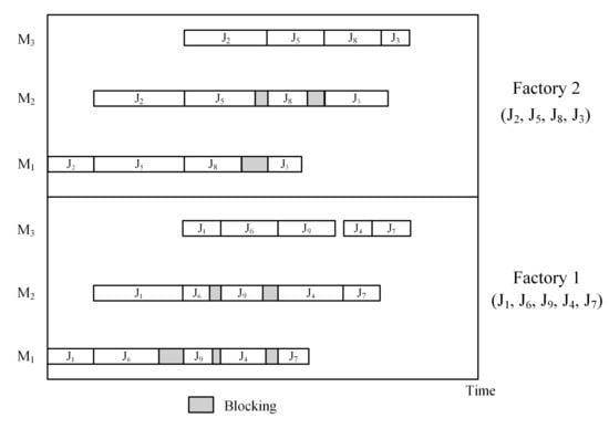
Figure 1.
Example of a Gantt chart for DBFSP with two factories.
Compared with conventional BFSP, scheduling in a distributed system is more complicated. In a single factory, jobs only need to be sequenced on a set of machines, whereas for DBFSP, an additional decision is especially required to determine the assignment of jobs to each factory. Apparently, both problems are highly related and cannot be solved without considering the sequential characteristics. Since has been verified to be NP-hard, even only for two machines [4], DBFSP is also NP-hard. Consequently, the traditional exact algorithms are not effective and applicable. For solving such complex and comprehensive scheduling problems, there is an urgent need for an effective yet simple algorithm with efficiency.
Bearing the above observations, this paper aims to tackle DBFSP with makespan criterion using a novel and effective discrete fruit fly optimization algorithm (DFOA). The proposed algorithm makes the following contributions:
- (1)
- An initialization strategy based on problem-specific characteristics is proposed to generate an initial population with good quality and diversity.
- (2)
- In the smell-based search phase of DFOA, a novel neighborhood strategy is designed with the view of extending the exploration.
- (3)
- To enhance the exploitation of DFOA, an adaptive VND-based local search strategy is highlighted.
- (4)
- In the vision-based search phase, an effective elite-based update criterion is proposed, which helps DFOA converge faster.
The rest of the components of this paper are outlined as follows. Section 2 systematically reviews the relevant literature. Section 3 states the DBFSP. The details of DFOA are presented in Section 4. Section 5 provides the numerical experiments and statistical analysis. The conclusions and future work are summarized in Section 6.
2. Related Work
To the best of our knowledge, few literature investigations have studied DBFSP. Thus, recent publications relevant to this paper are mainly concerned with the following three research streams: BFSP, distributed flowshop scheduling problem (DFSP), and fruit fly algorithm (FOA). In this section, the correlative literature is concluded.
2.1. Blocking Flowshop Scheduling Problem (BFSP)
BFSP is encountered in a rather wide range of industrial sectors, such as iron [5], chemical and gear industries [6], just-in-time production lines and in-line robotic cells [7], and computing resource management [8]. The optimal solution for BFSP can be harvested through exact algorithms, such as integer programming or brunch and bound. However, they are limited to small instances due to computational complexity. Therefore, recent research has focused on heuristics (including constructive and improvements heuristics) or metaheuristics. Heuristics completes the solution on a partial sequence or makes improvement according to the problem-specific characteristics, while metaheuristics is a combination of stochastic mechanism and local search algorithms [9]. Heuristics terminates spontaneously after a given number of steps regardless of the time limit [10], yet metaheuristics takes certain termination criterion as inputs. Moreover, metaheuristics usually needs fast initial solutions, of which the quality is known to affect the performance of the metaheuristics, to begin the search process. Hence, the initial solutions for the metaheuristics are often provided by heuristics.
In 2001, Caraffa et al. [11] proposed a genetic algorithm to solve BFSP with a makespan criterion. In 2007, Grabowski and Pempera [12] used a Tabu search (TS) algorithm to tackle the same problem. The experimental results demonstrated that TS was superior to GA. After that, Wang et al. [13] presented a hybrid discrete differential evolution algorithm (HDDE) for BFSP. The HDDE was proven to be more effective and efficient than algorithms in previous literature. Later, Ribas et al. [14] presented a simple yet effective iterated greedy (IG) algorithm combining with the NEH method [15]. In 2012, a discrete particle swarm algorithm (DPSO) [16] and an improved discrete artificial bee colony (IABC) algorithm [17] were proposed. Han et al. [18] further proposed a discrete artificial bee colony (DABC) incorporating a differential evolution (DE) strategy in 2015. In 2016, Han et al. [19] applied a novel FOA to solve BFSP and the results reported that 67 out of 90 new upper bounds of the Taillard benchmark [20] were improved. Recently, Shao et al. [21] proposed a novel discrete invasive weed optimization for BFSP.
2.2. Distributed Flowshop Scheduling Problem (DFSP)
DFSP is more complicated than the traditional FSP since there is an additional decision for job-to-factory assignment in the solution space. This problem-specific characteristic also requires a counter-change on the neighborhood search strategy and the optimization procedure. Naderi et al. [22] addressed DFSP for the first time in 2010. The authors developed six alternative mixed integer linear programming (MILP) models and 12 dispatching-based heuristics with two effective job-to-factory assignment rules. These two rules are described as follows:
- (1)
- Assign job j to the factory with the lowest current makespan Cmax (not including job j).
- (2)
- Assign job j to the factory that completes it at the earliest time, i.e., the factory resulting in the lowest makespan Cmax (after assigning job j).
Moreover, two iterative methods based on variable neighborhood descent (VND) [23] are proposed to search for better neighborhoods of the solution. Following this pioneering work, several approaches were surveyed and applied for DFSP, such as electromagnetism-like mechanism algorithm [24], hybrid genetic algorithm [25], Tabu search algorithm [26], estimation of distribution algorithm [27], scatter search algorithm [28], immune algorithm [29], chemical reaction optimization algorithm [30], and iterated greedy algorithm [31,32]. It is worth noting that Fernandez et al. [33] investigated DFSP with the total flow time (TFT) criterion for the first time in 2015. The authors also presented six job-to-factory assignment rules that were highly related to TFT and tested the performances of the rules in the experiments.
DBFSP is developed from DFSP by extending the permutation constraint to blocking. Heretofore, few literatures have focused on this field. Zhang et al. [34] designed a discrete differential evolution algorithm in 2018. Except for the DBFSP, Shao et al. [35] optimized the distributed no-wait flowshop scheduling problem (DNWFSP) with an improved IG algorithm for the first time.
2.3. Fruit Fly Algorithm (FOA)
FOA is a novel nature-inspired evolutionary algorithm proposed by Pan [36]. It is inspired by the foraging behavior of fruit fly swarms using sensitive osphresis and version. A fruit fly has two important organs, the olfactory and visual organs. The olfactory organ is used for smelling all types of odor in the air so that the fruit fly can fly towards the target locations. Afterward, it flies towards the food source with the help of the visual organ. The foraging behavior process of a fruit fly swarm is shown in Figure 2.
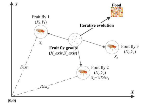
Figure 2.
Graphical presentation of foraging behavior of a fruit fly swarm.
According to the algorithm structure, FOA has two search phases, as follows: The smell-based search phase and the vision-based search phase. This parallel search framework enables the researchers to embed a number of heuristics, local search strategies, and solution generation operators in it, so that the exploration and exploitation of the framework can be enhanced. Compared with other metaheuristics, FOA is simple and has few parameters to implement. The experiment results from many literature examples have reported that FOA is competitive and appropriate for optimization problems. The searching procedure of FOA is outlined in the following steps:
- Step 1.
- Initialization of parameters: Set the population size and the number of generations.
- Step 2.
- Initialization of the fruit fly population with location.
- Step 3.
- Smell-based search phase: The fruit fly exploits N locations (i.e., food sources) randomly. Evaluate the N locations with the smell concentration values as fitness values.
- Step 4.
- Vision-based search phase: Replace the current best population location when a better location is found. The population flies towards the new best location.
- Step 5.
- Termination criterion: End the procedure if the maximum generation number is reached; otherwise, back to Step 3. The detailed search procedure of FOA refers to Reference [36].
Heretofore, FOA has been successfully applied to a variety of fields, including antenna arrays synthesis [37], traffic flow forecasting [38], web auction logistics [39], and multidimensional knapsack problems [40]. For scheduling problems, FOA was modified by Zheng et al. [41] to solve the semiconductor final testing scheduling problem, which can be abstracted as a flexible job shop scheduling problem (FJSP) with setup time and resource allocation constraints. Later, Zheng et al. [42] adopted a modified FOA to address the FJSP with dual resource constraints. The authors embedded the knowledge system into FOA so that the fruit fly can be guided towards the food source quickly in the vision-based search phase. Li et al. [43] proposed a hybrid FOA with an adaptive neighborhood strategy for scheduling problems in a steelmaking factory, where machine breakdown and disruptions were considered in real life.
2.4. Discussion
Although various approaches were developed to tackle the scheduling problems in distributed environments, there are the following observations in the considered fields. First, a majority of current literature focuses on DFSP and the variants of DFSP have not been fully investigated. Second, the increasing number of jobs will bring a huge obstacle when scheduling in a complex distributed environment. When solving DBFSP, it is better to apply a simple and effective algorithm with few parameters and low mathematical requirements.
With the above motivations, this paper presents a novel DFOA to solve DBFSP in a discrete manner. To the best of our knowledge, FOA has not been applied to DBFSP. In the proposed DFOA framework, a central location for the fruit fly population is generated in the initialization phase firstly. In the smell-based search phase, it is expected that the individual fruit fly can search in a random direction (neighborhood structure) around the center location in the decision space. When a fruit fly is getting close to a new location, a local search strategy is emphasized to guide it towards the best location. In the vision-based search phase, the aim of the algorithm is to guide the population to a better searching space quickly.
3. Problem Statement
In this section, we state DBFSP on the basis of BFSP. The derivation procedure of makespan is discussed.
3.1. Problem Description of BFSP and DBFSP
BFSP is described as follows. There is a job set consisting of n jobs and a machine set with m different machines. Each job will be sequentially processed on the machines 1, 2, …, m. The aim of solving BFSP is to minimize the makespan with a processing sequence. There are the following assumptions when solving BFSP:
- (1)
- The orders where all jobs to be processed is the same on each machine.
- (2)
- If is occupied, the job needs to be blocked on the current machine until is available.
- (3)
- The job cannot be interrupted once it starts operation.
- (4)
- Each machine can only handle one job at a time.
- (5)
- All jobs and machines are available at time zero.
- (6)
- The setup time of jobs is included in the processing time.
Based on BFSP, DBFSP considers processing n jobs by using a factory set , where . It is worth noting that all the factories in this study have the same machine configuration and environment. Jobs are not allowed to be removed to any other factories once they are processed in the assigned factory. A complete solution of DBFSP includes two correlative decisions, assigning jobs to factories and sequencing jobs in each factory. Let Cmax be the makespan in any of the factories. The aim of solving DBFSP in this paper is to minimize Cmax.
3.2. Mathematical Model of DBFSP
Let represent the partial sequence of jobs that are assigned to factory . Hence, a complete solution of DBFSP with F factories and n jobs can be presented as a set of partial sequences of all factories, i.e., . Assume that represents the departure time of operation on the machine i with the corresponding processing time . The value represents the start time of job on the first machine. In factory , can be deduced with the following recursive formulas:
where Equations (1) and (2) calculate the start and departure time of the first job from machine 1 to machine m. Equations (3) and (4) represent the start and departure time of job from machine 1 to machine m − 1. Equation (5) gives the departure time of job on the last machine m. By comparing the makespan of each factory , the objective function for DBFSP can be expressed as follows:
To clearly illustrate the deduction procedure, a makespan derivation procedure of a certain factory is provided as an example.
Example 1.
Assume that n (n > 4) jobs need to be processed. Firstly, they are assigned to F factories, each of which contains 3 machines. A job sequence() is given to factory. The processing timeof each job on each machine is shown as follows:
The departure timeis deduced as follows:
Finally, the makespan ofjobs processed in the factoryis.
4. Proposed Algorithm for Solving DBFSP
Although FOA has presented good performances on many engineering optimization problems, difficulties are still exposed when applying it to solving the scheduling problems. Firstly, due to the problem-specific discreteness, the continuous fitness functions in FOA cannot be directly employed and dedicated encoding and decoding schemes are necessary. Secondly, the random initialization mechanism of basic FOA reduces the quality of solutions, which further increases the difficulty in searching for the optimum value. Thirdly, the random search behavior of each fruit fly could not support the convergence performance of the population. Lastly, it misses an effective local search method to guide the fruit fly towards the best location.
To cope with the above limitations, we present a DFOA that inherits and extends the searching idea of basic FOA. The flowchart is presented in Figure 3. In the smell-based search phase, the algorithm explores the solution space. The VND-based local search aims to exploit the search space. In the vision-based search phase, DFOA updates the population with the best fruit fly found so far. DFOA balances both the exploration and exploitation. It is expected to achieve satisfactory performances for solving DBFSP.
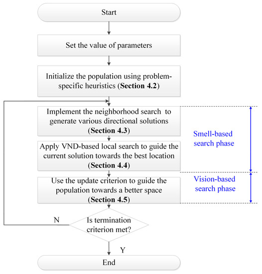
Figure 3.
Flow chart of the proposed DFOA.
4.1. Solution Representation
Based on the description from Section 3, the solution for DBFSP with factories and jobs can be defined as a set of partial sequences of all factories, as follows:
where denotes the partial sequence with jobs assigned in the factory , and . Such representation can be easily decoded to a DBFSP schedule because determines not only the processing sequence, but also the assigned jobs in factory .
Example 2.
A solution for DBFSP with n = 6 and F = 2 is considered. Hence, a complete solution is, where, and. When applying the decoding scheme, jobs J2, J1, and J6 are assigned to factory 1 and processed in the order of J2→J1→J6. The decoding procedure foris the same.
4.2. Population Initialization
When initializing the population, the decision of assigning jobs to factories should be considered. In this paper, the assignment rule implemented by Naderi and Ruiz [22], called the earliest completion factory (ECF) rule [26] is adopted. The pseudocode of the ECF rule is presented in Algorithm 1. ECF firstly arranges all the jobs according to their total processing time. Then, it assigns job j to the factory orderly that completes it at the earliest time, i.e., the lowest Cmax after including this job as the last job. This assignment rule was proven to be more effective than other rules for makespan minimization [28,33]. In addition, the decoding rule can also balance the workload between all factories. Based on the ECF rule, three heuristic initialization methods are proposed as follows: A distributed NEH-PWT method (DNPM), a distributed NEH method (NEH2) [22] and a distributed NEH random method (DNRM).
| Algorithm 1 ECF rule |
| Procedure ECF rule |
| Input Parameter (solution , factory number F) |
| Fork = 1 to F |
| End For |
| Fork = F + 1 to n |
| Find the factory f that can process job with the earliest completion time |
| End For |
| Output |
DNPM: The NEH heuristic approach [15] has proven to be one of the most effective heuristics known for FSP. The NEH method requires that the job with the larger total processing time should be arranged with a higher priority than the one with the smaller total processing time. Nevertheless, it may be unsuitable for scheduling problems with blocking or buffer constraints due to the problem-specific characteristics. For BFSP, arranging the job with the larger total processing time in the forepart of a permutation may lead to a larger blocking time for its successive jobs. The increased blocking time can cause a larger makespan value.
In response to this problem, Pan et al. have proposed the NEH-PWT method [13], which gives the job with shorter total processing time higher priority when sequencing. The NEH-PWT method was proven to be more superior to NEH for solving BFSP through the numerical experiments. Inspired by the idea, we apply the NEH-PWT method to construct DNPM, which contains the three following steps: First, all jobs to be processed are arranged in ascending order according to their total processing time, , to generate a job sequence, . Then, F partial sequences are constructed for all factories. With the ECF rule, insert each job from J1, J2, until Jn to all possible slots of all factories until the lowest makespan Cmax is found.
NEH2: The procedure of the NEH2 method is similar to DNPM, except that the job sequence, , is arranged in descending order according to their total processing time .
DNRM: The procedure of DNRM is similar to DNPM, except that the job sequence is generated through randomly arranging the order of jobs.
In the initialization phase, the fruit fly population with Ps individuals are produced with the above three heuristic methods. To guarantee the quality of solutions while keeping the diversity of the population, one solution is generated using DNPM, one is produced using NEH2, and the rest Ps-2 solutions are generated using DNRM.
4.3. Smell-Based Search Phase
In the smell-based search phase, each fruit fly searches for a food source in a random direction and generates a new location. The best location will be found and the whole population flies towards it. In this section, a neighborhood search strategy that contains four solution generation operators is proposed to help a fruit fly find a good location in its local region. A neighborhood structure is defined by representing the way it modifies the incumbent feasible solution to determine a new feasible solution. The design of neighborhoods in a distributed environment needs to consider the fact that the global makespan cannot be improved without involving the factory with the largest makespan (defined as critical factory ). That is, it makes no sense, when the neighborhood search strategy is implemented within a non-critical factory or between two non-critical factories. Considering such characteristics, we exploit the neighborhood structures within the critical factory, as well as between the critical factory and other factories.
The solution generation operators are classified into two categories, as follows: One is based on the job sequence adjustment, including forward insertion and backward insertion within the critical factory; another one is based on the reassignment of jobs, including insertion and the swap between the critical factory and other factories. The four solution generation operators are depicted as follows. An example of the four solution generation operators is given in Figure 4.
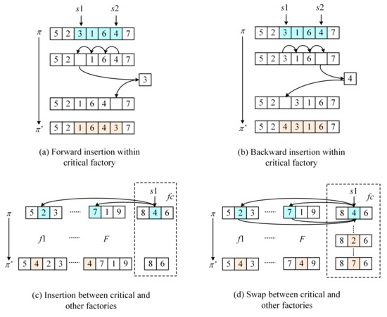
Figure 4.
Solution generation operators of the neighborhood structures.
Forward insertion within the critical factory : Stochastically select one if there is more than one critical factory. Choose two positions, s1 and s2 (s2 > s1), at random. The block between these two positions is referred to B1. Move B1 and s2 one position forward by turns, move s1 to the original position of s2 (please see Figure 4a).
Backward insertion within the critical factory : Choose two positions, s1 and s2 (s2 > s1), at random. The block between these two positions is referred to as B1; move B1 and s1 one position forward by turns, move s2 to the original position of s1 (please see Figure 4b).
Insertion between and other factories: Randomly select one job, J, at position s1 in the . For each of the other F − 1 factories, randomly select one position and insert J to this position. Thus, F − 1 solutions are generated. Choose the best one (with lowest global makespan) as the candidate solution. (please see Figure 4c).
Swap between and other factories: Randomly select one job J at position s1 in the . For each of the other F − 1 factories, randomly select one job and swap J and J*. Then, F − 1 solutions are generated. Choose the best one as the candidate solution. (please see Figure 4d).
The pseudocode of the neighborhood search strategy is sketched in Algorithm 2. In general, more operators can enhance the search ability of the individual in a higher probability than a single one. This strategy also holds the diversity of the population. After generating the neighborhood structures, the candidate solutions are evaluated. The best one is considered as the new solution to undergo the local search, which aims to conduct the new solution rapidly towards the best location.
| Algorithm 2 Neighborhood search strategy |
| Procedure Neighborhood search strategy |
| Input: Parameter (initialized solution , critical factory fc) Output: Solution |
| Begin // neighborhood operation |
| :← Forward insertion operator within the critical factory :← Backward insertion operator within the critical factory :← Insertion operator between the critical factory and other factories :← Swap operator between the critical factory and other factories evaluate , , , // makespan evaluation Output End |
4.4. VND-Based Local Search
During the procedure of FOA iteration, the whole population gathers around the best location. Each individual can only learn from the current optimal individual. This makes the algorithm very easy to trap into the local optimum. To overcome such premature problems, FOA needs to furnish with a mechanism that helps escape from the local optimum and continue searching in other solution spaces.
In most BFSP literature, insertion and swap movements are universally recognized as effective and efficient search processes to produce better solutions. Following this vein, a local search scheme based on insertion and swap variants of the VND method [23] is embedded in the proposed algorithm. VND is a variant of variable neighborhood search (VNS), where N neighborhood structures are systematically switched in a definitive way. VND begins from the first neighborhood and undergoes the improvement procedures until a local optimum in relation to all neighborhoods is reached. When no further improvement for the current neighborhood is obtained and , the search procedure carries on with the neighborhood. Like VNS, if a better solution is found, VND starts again from the first neighborhood. When , the search procedure terminates and rewards the final solution. VND is simple and easy to implement and it has shown high performances for many optimization problems. In this section, the concept of VND is adopted in the local search part to help the algorithm explore a larger solution space. Following the design philosophy of neighborhood structure in Section 4.3, and to avoid redundant computing procedures, two neighborhood movements for the VND are proposed. The insertion (LS_Insert) and swap movement (LS_Swap) are presented as follows.
LS_Insert: Select a job j1 from the critical factory and insert it in the best position of a non-critical factory. The best position refers to the position that obtains the lowest makespan after insertion movement. The improvement is recognized if the makespan Cmax is diminished. The permutation of jobs in this factory is kept and the search procedure starts with the factory that now has the maximal makespan. If the movement cannot improve the makespan, select a new job, j2, from the original critical factory to rerun the procedure. The procedure terminates after traversing all jobs of the original critical factory. Moreover, to accelerate the insertion procedure, a modified speed-up method proposed by Reference [13] is adopted in this study. The speed-up method is applied to evaluate the partial sequences obtained by inserting one job, J, in all the possible positions of factory that already has assigned jobs. The speed-up method can reduce the time complexity from O(mn3) to O(mn2) for an insertion-based local search procedure, which is crucial for an algorithm with high performance. The detailed procedure is described as follows.
- Step 1:
- Calculate the departure time, , of the jobs that are already assigned in the factory with Equations (1)–(5).
- Step 2:
- Calculate the tails, , of jobs that are already assigned in the factory with Equations (9)–(13), shown as follows:
- Step 3:
- Calculate the departure times, , of jo J to be inserted in the position q of the selected factory in the current solution.
- Step 4:
- Compare the makespan of the selected factory after inserting job J in the position by
- Step 5:
- Choose the best insertion position and return the best makespan. The pseudocode of the LS_Insert process is illustrated in Algorithm 3.
LS_Swap: Select each job from the critical factory, swap j1 with all jobs of all non-critical factories orderly, and reinsert jobs in the best position of the new factories, i.e., the position that results in the lowest makespan. The improvement is recognized if the makespan Cmax is diminished. The procedure terminates after all jobs of the critical factory have been selected. The speed-up method used for LS_Swap is the same as one used for LS_Insert, except that a job is removed from the original factory before a new job can be inserted. The LS_Swap process is described in Algorithm 4. Moreover, the pseudocode of the VND local search scheme is illustrated in Algorithm 5.
| Algorithm 3 Local search insert |
| Procedure Local search insert |
| Input: Parameter (solution , factory number F) |
| Output: Solution |
| Begin |
| While stop criterion is not satisfied |
| For j = 1 to // traverse all jobs in the critical factory |
| Select job j from the critical factory fc without repetition |
| Select a factory f randomly without repetition (with sequence ) |
| Insert j in the best position of f and obtaining |
| If then |
| : update by substituting with , remove job j from the critical factory |
| Calculate the using the speed-up method and detect the new critical factory |
| Else |
| End If |
| End For |
| End While |
| End |
| Algorithm 4 Local search swap |
| Procedure Local search swap |
| Input: Parameter (solution , factory number F) |
| Output: Solution |
| Begin |
| While the stop criterion is not satisfied |
| For j = 1 to // job number in the critical number |
| Select j from the critical factory fc without repetition |
| For f = 1 to F // select a non-critical factory |
| If f ≠ fc then |
| For i = 1 to // the job number in the select factory |
| remove job j from fc and insert i in the best position of fc obtaining , calculate using the speed-up method |
| remove job i from f and insert j in the best position of f obtaining , calculate using the speed-up method |
| If and then |
| : modify with and |
| Else , return job j and job i to their original positions |
| End If |
| End For |
| End If |
| End For |
| End For |
| Output |
| End |
| Algorithm 5 VND-based local search |
| Procedure VND-based local search |
| Input: Parameter (Solution ) |
| Output: Solution |
| Begin |
| Nl = {LS_Insert, LS_Swap} |
| For i = 1 to Size(Nl) |
| If then |
| Else i = i + 1 End If |
| If i > Size(Nl) |
| Break End If End For |
| End |
4.5. Vision-Based Search Phase
The purpose of the vision-based search phase is to guide the fruit fly population to fly towards a superior space to further enhance the performance of the proposed algorithm. An elite-based update criterion is applied in this study. Firstly, retrieve the whole population and find the individual with the largest makespan. Secondly, replace it with the individual with lowest makespan found so far. After the vision-based search phase, DFOA finishes one iteration. The search procedure repeats until the termination criterion is reached. The pseudocode of DFOA is illustrated in Algorithm 6. The complexity of the algorithm is .
| Algorithm 6 DFOA for DBFSP |
| Procedure DFOA for DBFSP |
| Input: Parameter (population size Ps, termination time Tmax) |
| Output: best solution |
| Begin |
| // Initialize population (Section 4.2) |
| ← problem-specific heuristic (DNPM) |
| ← problem-specific heuristic (NEH2) |
| ← problem-specific heuristic (DNRM) |
| Repeat |
| Fori = 1 to Ps // smell-based search phase (Section 4.3) |
| ← Neighborhood search strategy |
| ← VND-based local search // (Section 4.4) |
| If then |
| If then |
| End If |
| End If |
| End For |
| // vision-based search phase (Section 4.5) |
| Find out the worst solution in the whole population |
| = Update criterion () |
| Until the termination time Tmax is met |
| End |
5. Computational Experiment
5.1. Experiment Setting
Since there are no dedicated instances available, as a compromise, the computational experiments were conducted with the benchmark for DFSP modified by Naderi and Ruiz [28], which is extended from the benchmark of Taillard [20]. The benchmark comprises a set of 420 small instances (developed in 2010) and a set of 720 larger instances (developed in 2014).
Moreover, the authors appended two sets (small and large) of 50 test instances for calibration with n, m, and f values randomly sampled from the set of 720 instances. To be more specific, the benchmark contained 72 sets of 10 instances ranging from 20 jobs × 5 machines to 500 jobs × 20 machines, where n ϵ {20, 50, 100, 200, 500} and m ϵ {5, 10, 20}. The number of factories, f, is in the set {2, 3, 4, 5, 6, 7}. All instances are available on http://soa.iti.es.
In order to evaluate the effectiveness of proposed DFOA in different domains, it was compared with other heuristics and metaheuristics. In the experiment, the same experimental environment, including hardware, programming language, and termination criterion were applied. All the algorithms were coded in Python and loaded on a PC with an Intel(R) Core(TM) i7-8700 CPU and 16G RAM. The termination criterion for each compared metaheuristic was set as the maximal elapsed CPU time Tmax = n × m × F × 90 milliseconds (ms). Setting this CPU time correlated with the instance size and computational complexity enables the test algorithm to have more time to address large-scale instances that may be “hard” [44]. The generated minimum makespan is recorded for calculation of the statistical indicators. Denote as the solution provided by the r-th running of the i-th compared algorithm and represents the best solution obtained by any of the algorithms. To estimate the computational results, the following statistical indicators are computed:
- (1)
- Average relative percentage deviation (ARPD) is considered as a response variable that evaluates the mean quality of solutions, as follows:
- (2)
- Standard deviation (SD) that evaluates the quality of initial solutions and the robustness of the algorithm, as follows:
From Equation (15) it is clear that the lower the ARPD value is, the better is the compared algorithm performance. The experiments are conducted considering following aspects:
- (1)
- Sensitivity analysis of parameter Ps;
- (2)
- Comparison of the heuristics initialization methods;
- (3)
- Comparison of the local search methods;
- (4)
- Comparison with heuristics on small-scale instances;
- (5)
- Comparison with metaheuristics from other literature on large-scale instances.
5.2. Sensitivity Analysis
As mentioned, one advantage of DFOA is its simplicity. Compared with other algorithms, FOA has only few parameters to adjust. Here, a sensitivity analysis of the parameter population size (Ps) is conducted on the test instances. According to usual practice, a small value of Ps brings the algorithm an insufficient search and convergence ability. On the contrary, a large value of Ps can obtain better results because more fruit flies increase the diversity and can explore more locations in the solution space. However, an overlarge value will yield a high computational cost. As a trade-off, Ps was set as 35 according to the sensitivity analysis, which is shown in Figure 5.
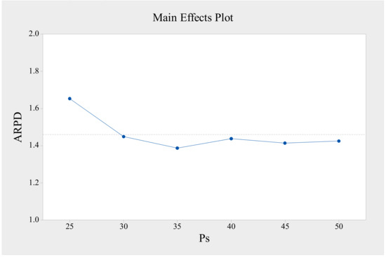
Figure 5.
Sensitivity analysis of parameter Ps.
5.3. Comparison of the Heuristic Initialization Methods
To analyze the effectiveness of the heuristic initialization methods in Section 4.2, DNPM, NEH2, and DNRMwe tested separately. All of them are heuristics that need no termination criterions for implementation. However, due to randomness, DNRM, especially, was repeated 10 times and the average value is taken as the test result. The comparison results are listed in the form of ARPD values in Table 1, grouped by different factory numbers. Note that the result of each group is the average value of all test instances in this group. In Table 1, the best performing heuristic was DNPM, with 13.86 on average, and it produced smaller ARPD values for all factories. The second best heuristic was NEH2, which produced an average ARPD value of 15.87. The DNRM yielded the worst results by a value of 22.41, on average. From these results, we confirmed that the DNPM is more suitable for DBFSP. It also indicates that the blocking constrains areas different from the permutation constraints, which reminds the researchers to design dedicated methods to handle it.

Table 1.
The comparison results of DNRM, NEH2, and DNPM in the algorithm.
In addition, Figure 6a presents the mean plot, with a 95% confidence interval, of the three heuristics. It is clear that the overall ARPDs of DNPM stayed under NEH2 and DNRM without any overlapping for all factories, which reports that the DNPM performed significantly better than the NEH2 and DNRM from the statistical view. On the other hand, in Figure 6b, we can observe the behavior of the initialization methods with the size of the instances (n × m). As seen, the most influential factor is the number of machines in each factory. With the increment of m, the performances of all the initialization methods improved.
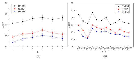
Figure 6.
(a) Mean plot with 95% confidence interval of interaction between the initialization methods and factories; (b) ARPD values by different initialization methods, with m × n.
5.4. Comparison of the Local Search Methods
In this section, the performances of the proposed local search methods are compared. DFOA was used as the test algorithm. For a fair comparison, the initialization methods applied are the same. That is, to overcome the randomness brought by DNRM, DFOA generates the Ps − 2 solutions by DNRM only once, they are applied for all the compared metaheuristics. Consequently, four metaheuristics are created, i.e., DFOA + LS_Insert (with LS_ins for short), DFOA + LS_Swap (with LS_sw for short), DFOA + no local search (with NLS for short), and DFOA + VND (with LS_V for short). Table 2 lists the ARPD values for all algorithms, grouped by different factory numbers.
Table 2.
The Comparison results of LS_ins, LS_sw, NLS and LS_V in the algorithm.
As seen in Table 2, between LS_ins and LS_sw, LS_sw achieved better performance, with an overall ARPD value of 1.302, while the LS_ins obtained the overall ARPD value of 1.518. This demonstrates that the exploitation ability of LS_sw is relatively stronger. In most literature, the insertion movement explores larger searching spaces than the swap movement. In this experiment, however, the swap operation attached the insertion procedure after the swap movement and produced thereby better results. Additionally, the overall ARPD value of LS_V is 0.847, which shows large superiority over the results provided by the other three metaheuristics. This indicates that a better performance can be obtained by combining multiple local search methods. Since different local search methods explore different solution spaces, a hybridization strategy can help escape the local optimum. It is not surprising that, among the four metaheuristics, NLS obtained the worst performance, with an overall ARPD value of 2.154. Like some other nature-inspired algorithms, FOA has a better exploration ability but with a poor exploitation ability. An embedded local search could overcome this limitation.
Figure 7 illustrates the mean plot, with a 95% confidence level, between the compared local search methods and factory numbers. As can be seen, LS_sw gained slightly better results than LS_ins, but the differences between them are not large enough to define the significant difference from a statistical view. The overall ARPD values of LS_V lie totally under those of LS_ins, LS_sw, and NLS without overlapping, which indicates that LS_V is significantly better than the other three metaheuristics.
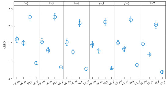
Figure 7.
Mean plot with a 95% confidence interval of the interaction between local search methods and factories.
5.5. Comparison with Heuristics on Small-Scale Instances
In this section, the proposed algorithm is compared with some constructive heuristics proposed by Naderi and Ruiz in 2010 [22]. The authors have developed largest processing time heuristics (LPT2), shortest processing time heuristics (SPT2), heuristic by Johnson’s rule (Johnson2), and heuristics of NEH2 and VND(a). The suffix “2” means that the second job-to-factory rule is employed, which was proven to be more effective than the first one proposed in their studies. More details about the test algorithms refer to Reference [22]. The 420 small-scale instances are used to compare DFOA with the above five heuristics. All the results are grouped by each combination of the factory number, F, and the number of jobs, n. Each group contains 20 instances. The result of each group is the average result from 20 instances. The termination criterion for DFOA is 50 iterations. From Table 3 it can be seen that DFOA is the best algorithm for solving the small-scale instances. VND(a) ranks second and the NEH2 method ranks third. LPT2 and Johnson2 obtained the largest ARPD (21.027) and the second largest ARPD (13.933), respectively. The performance comparison between LPT2 and SPT2 also reflects the problem-specific characteristics of DBFSP, which has an inverse relation when both of them are applied for DFSP.
Table 3.
ARPD values by different algorithms on small-scale instances.
In addition, we come to the following conclusion. (1) The instance combination F × n = 4 × 4 gives no other arrangement on the solution. Hence, the results obtained by all algorithms were the same. (2) When the complexity of the combination increased, the ARPD values increased as well. (3) It is clear that the results obtained by heuristics are far from those of metaheuristics. However, heuristics has the advantage on CPU time. Table 4 demonstrates the time consumptions of all the compared algorithms. As seen, the CPU time is especially small when applying the constructive heuristics, whereas metaheuristics consume more time due to their iterated procedure. Since our aim is to minimize the makespan, this CPU time can be accepted in practice use. It was also found that CPU time reduces with the increment of the factory number F, which indicates that the instance becomes easier to solve when F becomes larger.
Table 4.
Average time consumptions (s) on small-scale instances grouped by factory number F.
5.6. Comparison to Other Metaheuristics on Large-Scale Instances
In this section, DFOA is compared with the well-known metaheuristics on large-scale instances. Since there is little literature published for DBFSP so far, some metaheuristics from DFSP literature are modified and applied for the DBFSP. The compared metaheuristics are the following: (1) The discrete electromagnetism-like mechanism algorithm (EM) of Liu et al. [24]; (2) the hybrid genetic algorithm (HGA) of Gao et al. [25], (3) the Tabu search (TS) of Gao et al. [26]; and (4) the discrete differential evolution algorithm (DDE) of Zhang et al. [34]. Not all metaheuristics in the reviewed literature are compared, as some of them are hard to replicate without accessing their original codes. Since all metaheuristics perform well and have a strong search ability, the comparison differences on the small-scale instances are not significant. Hence, only the comparison results on the large-scale instances are demonstrated.
Given the five algorithms tested, 720 large-scale benchmark instances and 10 replications, there are, in total, 36,000 results. It is worth mentioning that we strictly complied with the detailed description of the literature to carry out the above metaheuristics. Even though most of them were not originally developed for DBFSP, their searching essences (e.g., the architecture, the encoding and decoding scheme, the local search method) were not abandoned. Only the fitness functions are adjusted to match the problem considered. The parameters of the compared metaheuristics are listed in Table 5.
Table 5.
Parameter setting of the compared algorithms.
In order to investigate the differences and performance trends between the above metaheuristics comprehensively, the results in Table 6 were grouped by the influential factors, i.e., the number of factories, F, jobs, n, and machines, m, respectively. As seen, DFOA obtained the lowest ARPD values in all instances by all factors. The overall ARPD of DFOA was 0.91, which is remarkably better than that of EM (4.985), HGA (3.202), TS (2.901), and DDE (1.548).
Table 6.
Algorithmic comparison on large-scale instances, grouped by different factors.
For the instances grouped by F, n, and m, the performance trends of metaheuristics are presented in Figure 8. From Figure 8a it can be seen that the entire performances of all metaheuristics improved with the increment of F, when the value of F was over five. It also indicates that a small factory number would not dominate their performances as expected. The algorithmic performances fluctuate when F is smaller than five. Other influential factors such as job number n, machine number m, or the algorithmic components like population size, may interfere with the performances more comprehensively. In Figure 8b, it is clear that with the increment of n, the performances of the metaheuristics became worse in general. This may because assigning more jobs to fixed machines makes the situation more complicated and results in more blocking situations. The same argument is suggested for the performance trends that were grouped by different machine numbers, which is shown in Figure 8c.
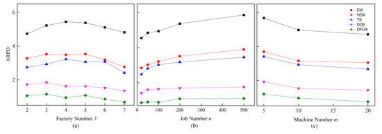
Figure 8.
Performance trends of metaheuristics on different: (a) Factory number; (b) job number; and (c) machine number.
Figure 9, Figure 10 and Figure 11 demonstrate three typical convergence curves of the compared metaheuristics on different instances. As can be seen, with the increment of computation complexity, the differences between metaheuristics become larger.
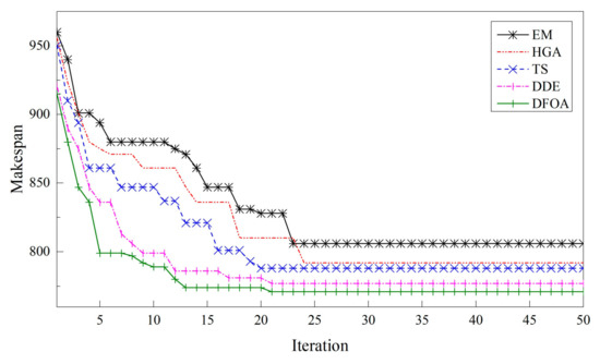
Figure 9.
Convergence curves of instance Ta001_2.
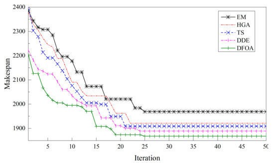
Figure 10.
Convergence curves of instance Ta101_6.
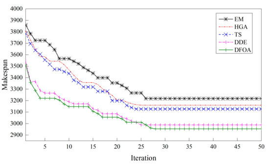
Figure 11.
Convergence curves of instance Ta110_7.
Furthermore, Holm’s multi-test [45] was adopted to evaluate the comparison between different metaheuristics. In Holm’s method, represent m hypotheses and are the corresponding p-values, which denote the probabilities of observing the given results by chance. The p-values are ordered from lowest to highest by . For a given significance level , let k be the minimal index so that . As a result, the null hypotheses from to will be rejected and the hypotheses from to will be accepted. As seen in Table 7, the returned p-values for all groups of hypotheses were zero. According to Holm’s method, all the hypotheses were rejected. This confirms the statistical differences in the favor of DFOA over other metaheuristics.
Table 7.
Holm’s multi-test for all compared metaheuristics.
In the above paragraphs, the effectiveness of the proposed DFOA was tested and compared with the known existing metaheuristics. It can be concluded that DFOA is more effective than other metaheuristics when solving DBFSP with makespan criterion. The advantages are attributed to the delicate-designed algorithmic components according to the problem-specific characteristics as well as their suitable hybridization.
6. Conclusion and Future Works
In this study, a discrete fruit fly optimization algorithm (DFOA) is proposed to solve the blocking flowshop scheduling problem (DBFSP) in a distributed manufacturing system. Firstly, the problem description of DBFSP and mathematical model are presented. To solve this problem, a problem-specific initialization strategy was designed to generate an initial fruit fly population with quality and diversity. In the smell-based search phase of DFOA, four neighborhood structures for each individual were designed and the one with the best performance was selected to generate a new location in a deterministic way. Later, a VND-based local search scheme was designed. This mechanism implements an exhaustive search, which is competent for enhancing the exploitation ability in the promising space. In the vision-based search phase of DFOA, an effective update criterion was applied. The experiments were conducted by comparing the proposed DFOA with well-known constructive heuristics and metaheuristics on small-scale and large-scale instances. The experimental results indicate that the proposed multiple-neighborhood strategy is conducive to enlarge the global search space. The performance of the proposed VND is proven to be more effective than single local search technology. Overall, the experiment results have shown that the proposed DFOA can handle DBFSP with a better search and optimization ability.
FOA has few parameters to be implemented, which can reduce the lengthy procedure of optimization. However, its simple structure still suffers from common problems (e.g., convergence precision) like other nature-inspired algorithms. Therefore, to overcome such deficiencies, future work will focus on the hybridization of the searching idea with other algorithms or strategies, such as PSO or knowledge-based systems.
On the other side, a multiobjective DBFSP is also considered, with the view of reaching a trade-off between energy consumption or carbon footprint and makespan.
Author Contributions
Conceptualization, S.T. and Z.L.; Methodology, X.Z., X.L., and G.K.; Software, X.Z and X.L.; Validation, X.Z., X.L., and Z.L.; Formal analysis, X.Z., X.L., and G.K.; Investigation, X.L. and S.T.; Writing—original draft preparation, X.Z. and X.L.; Writing—review and editing, G.K. and Z.L.; Supervision, S.T.; Project administration, X.L. and Z.L.
Funding
This research was funded by the Science and Technology Plan of Lianyungang (No. CG1615), Fundamental Research project of Central Universities (No. 201941008), Priority Academic Program Development of Jiangsu Higher Education Institutions (PAPD) and Australia ARC DECRA (No. DE190100931).
Acknowledgments
The authors would like to thank the anonymous reviewers for their contribution to this paper.
Conflicts of Interest
The authors declare no conflict of interest.
References
- Zhao, F.; Xue, F.; Zhang, Y.; Ma, W.; Zhang, C.; Song, H. A discrete gravitational search algorithm for the blocking flow shop problem with total flow time minimization. Appl. Intell. 2019, 49, 3362–3382. [Google Scholar] [CrossRef]
- Leisten, R. Flowshop sequencing problems with limited buffer storage. Int. J. Prod. Res. 1990, 28, 2085–2100. [Google Scholar] [CrossRef]
- Graham, R.L.; Lawler, E.L.; Lenstra, J.K.; Kan, A.R. Optimization and approximation in deterministic sequencing and scheduling: A survey. Ann. Discret. Math. 1979, 5, 287–326. [Google Scholar] [CrossRef]
- Riahi, V.; Newton, M.H.; Su, K.; Sattar, A. Constraint guided accelerated search for mixed blocking permutation flowshop scheduling. Comput. Oper. Res. 2019, 102, 102–120. [Google Scholar] [CrossRef]
- Nagano, M.S.; Komesu, A.S.; Miyata, H.H. An evolutionary clustering search for the total tardiness blocking flow shop problem. J. Intell. Manuf. 2019, 30, 1843–1857. [Google Scholar] [CrossRef]
- Leiras, A.; Hamacher, S.; Elkamel, A. Petroleum refinery operational planning using robust optimization. Eng. Optim. 2010, 42, 1119–1131. [Google Scholar] [CrossRef]
- Zhu, Q.; Wu, N.; Yan, Q.; Zhou, M. Optimal scheduling of complex multi-cluster tools based on timed resource-oriented petri nets. IEEE Access 2017, 4, 2096–2109. [Google Scholar] [CrossRef]
- Pan, D.; Yang, Y. Localized independent packet scheduling for buffered crossbar switches. IEEE Trans. Comput. 2009, 58, 260–274. [Google Scholar] [CrossRef]
- Fernandez-Viagas, V.; Leisten, R.; Framinan, J.M. A computational evaluation of constructive and improvement heuristics for the blocking flow shop to minimise total flowtime. Expert Syst. Appl. 2016, 61, 290–301. [Google Scholar] [CrossRef]
- Zhang, Y.; Gong, D.W.; Sun, J.Y.; Qu, B.Y. A decomposition-based archiving approach for multi-objective evolutionary optimization. Inf. Sci. 2018, 430, 397–413. [Google Scholar] [CrossRef]
- Caraffa, V.; Ianes, S.; Bagchi, T.P.; Sriskandarajah, C. Minimizing Makespan in a Blocking Flowshop using Genetic Algorithms. Int. J. Prod. Econ. 2001, 70, 101–115. [Google Scholar] [CrossRef]
- Grabowski, J.; Pempera, J. The permutation flow shop problem with blocking. A tabu search approach. Omega 2007, 35, 302–311. [Google Scholar] [CrossRef]
- Wang, L.; Pan, Q.K.; Suganthan, P.N.; Wang, W.H.; Wang, Y.M. A novel hybrid discrete differential evolution algorithm for blocking flowshop scheduling problems. Comput. Oper. Res. 2010, 37, 509–520. [Google Scholar] [CrossRef]
- Ribas, I.; Companys, R.; Tort-Martorell, X. An iterated greedy algorithm for the flowshop scheduling problem with blocking. Omega 2011, 39, 293–301. [Google Scholar] [CrossRef]
- Nawaz, M.; Enscore, E.E., Jr.; Ham, I. A heuristic algorithm for the m-machine, n-job flow-shop sequencing problem. Omega 1983, 11, 91–95. [Google Scholar] [CrossRef]
- Wang, X.; Tang, L. A discrete particle swarm optimization algorithm with self-adaptive diversity control for the permutation flowshop problem with blocking. Appl. Soft Comput. 2012, 12, 652–662. [Google Scholar] [CrossRef]
- Han, Y.Y.; Pan, Q.K.; Li, J.Q.; Sang, H.Y. An improved artificial bee colony algorithm for the blocking flowshop scheduling problem. Int. J. Adv. Manuf. Technol. 2012, 60, 1149–1159. [Google Scholar] [CrossRef]
- Han, Y.Y.; Gong, D.W.; Sun, X.Y.; Pan, Q.K. An improved NSGA-II algorithm for multi-objective lot-streaming flow shop scheduling problem. Int. J. Prod. Res. 2014, 52, 2211–2231. [Google Scholar] [CrossRef]
- Han, Y.Y.; Gong, D.W.; Li, J.Q.; Zhang, Y. Solving the blocking flowshop scheduling problem with makespan using a modified fruit fly optimisation algorithm. Int. J. Prod. Res. 2016, 54, 6782–6797. [Google Scholar] [CrossRef]
- Taillard, E. Benchmarks for basic scheduling problems. Eur. J. Oper. Res. 1993, 64, 278–285. [Google Scholar] [CrossRef]
- Shao, Z.; Pi, D.; Shao, W.; Yuan, P. An efficient discrete invasive weed optimization for blocking flow-shop scheduling problem. Eng. Appl. Artif. Intell. 2019, 78, 124–141. [Google Scholar] [CrossRef]
- Naderi, B.; Ruiz, R. The distributed permutation flowshop scheduling problem. Comput. Oper. Res. 2010, 37, 754–768. [Google Scholar] [CrossRef]
- Peng, K.; Pan, Q.K.; Gao, L.; Li, X.; Das, S.; Zhang, B. A multi-start variable neighbourhood descent algorithm for hybrid flowshop rescheduling. Swarm Evolut. Comput. 2019, 45, 92–112. [Google Scholar] [CrossRef]
- Liu, H.; Gao, L. A discrete electromagnetism-like mechanism algorithm for solving distributed permutation flowshop scheduling problem. In Proceedings of the International Conference on Manufacturing Automation, Hong Kong, China, 13–15 December 2010; pp. 156–163. [Google Scholar]
- Gao, J.; Chen, R. A hybrid genetic algorithm for the distributed permutation flowshop scheduling problem. Int. J. Comput. Int. Syst. 2011, 4, 497–508. [Google Scholar] [CrossRef]
- Gao, J.; Chen, R.; Deng, W. An efficient tabu search algorithm for the distributed permutation flowshop scheduling problem. Int. J. Prod. Res. 2013, 51, 641–651. [Google Scholar] [CrossRef]
- Wang, S.Y.; Wang, L.; Liu, M.; Xu, Y. An effective estimation of distribution algorithm for solving the distributed permutation flow-shop scheduling problem. Int. J. Prod. Econ. 2013, 145, 387–396. [Google Scholar] [CrossRef]
- Naderi, B.; Ruiz, R. A scatter search algorithm for the distributed permutation flowshop scheduling problem. Eur. J. Oper. Res. 2014, 239, 323–334. [Google Scholar] [CrossRef]
- Xu, Y.; Wang, L.; Wang, S.; Liu, M. An effective hybrid immune algorithm for solving the distributed permutation flow-shop scheduling problem. Eng. Optim. 2013, 46, 1269–1283. [Google Scholar] [CrossRef]
- Bargaoui, H.; Driss, O.B.; Ghedira, K. A novel chemical reaction optimization for the distributed permutation flowshop scheduling problem with makespan criterion. Comput. Ind. Eng. 2017, 111, 239–250. [Google Scholar] [CrossRef]
- Pan, Q.K.; Gao, L.; Wang, L.; Liang, J.; Li, X.Y. Effective heuristics and metaheuristics to minimize total flowtime for the distributed permutation flowshop problem. Expert Syst. Appl. 2019, 124, 309–324. [Google Scholar] [CrossRef]
- Ruiz, R.; Pan, Q.K.; Naderi, B. Iterated Greedy methods for the distributed permutation flowshop scheduling problem. Omega 2019, 83, 213–222. [Google Scholar] [CrossRef]
- Fernandez-Viagas, V.; Framinan, J.M. A bounded-search iterated greedy algorithm for the distributed permutation flowshop scheduling problem. Int. J. Prod. Res. 2015, 53, 1111–1123. [Google Scholar] [CrossRef]
- Zhang, G.; Xing, K.; Cao, F. Discrete differential evolution algorithm for distributed blocking flowshop scheduling with makespan criterion. Eng. Appl. Artif. Intell. 2018, 76, 96–107. [Google Scholar] [CrossRef]
- Shao, W.; Pi, D.; Shao, Z. Optimization of makespan for the distributed no-wait flow shop scheduling problem with iterated greedy algorithms. Knowl. Based Syst. 2017, 137, 163–181. [Google Scholar] [CrossRef]
- Pan, W.T. A new fruit fly optimization algorithm: Taking the financial distress model as an example. Knowl. Based Syst. 2012, 26, 69–74. [Google Scholar] [CrossRef]
- Darvish, A.; Ebrahimzadeh, A. Improved fruit-fly optimization algorithm and its applications in antenna arrays synthesis. IEEE Trans. Antennas Propag. 2018, 66, 1756–1766. [Google Scholar] [CrossRef]
- Cong, Y.; Wang, J.; Li, X. Traffic flow forecasting by a least squares support vector machine with a fruit fly optimization algorithm. Procedia Eng. 2016, 137, 59–68. [Google Scholar] [CrossRef]
- Lin, S.M. Analysis of service satisfaction in web auction logistics service using a combination of fruit fly optimization algorithm and general regression neural network. Neural Comput. Appl. 2013, 22, 783–791. [Google Scholar] [CrossRef]
- Meng, T.; Pan, Q.K. An improved fruit fly optimization algorithm for solving the multidimensional knapsack problem. Appl. Soft Comput. 2017, 50, 79–93. [Google Scholar] [CrossRef]
- Zheng, X.L.; Wang, L.; Wang, S.Y. A novel fruit fly optimization algorithm for the semiconductor final testing scheduling problem. Knowl. Based Syst. 2014, 57, 95–103. [Google Scholar] [CrossRef]
- Zheng, X.; Wang, L. A knowledge-guided fruit fly optimization algorithm for dual resource constrained flexible job-shop scheduling problem. Int. J. Prod. Res. 2018, 54, 1–13. [Google Scholar] [CrossRef]
- Li, J.Q.; Pan, Q.K.; Mao, K. A hybrid fruit fly optimization algorithm for the realistic hybrid flowshop rescheduling problem in steelmaking systems. IEEE Trans. Autom. Sci. Eng. 2016, 13, 932–949. [Google Scholar] [CrossRef]
- Deng, G.L.; Yu, H.Y.; Zheng, S.M. An enhanced discrete artificial bee colony algorithm to minimize the total flow time in permutation flowshop scheduling with limited buffers. Math. Probl. Eng. 2016, 2016, 1–11. [Google Scholar] [CrossRef]
- Holm, S. A simple sequentially rejective multiple test procedure. Scand. J. Stat. 1979, 6, 65–70. [Google Scholar] [CrossRef]
© 2019 by the authors. Licensee MDPI, Basel, Switzerland. This article is an open access article distributed under the terms and conditions of the Creative Commons Attribution (CC BY) license (http://creativecommons.org/licenses/by/4.0/).