Article

Load Areas in Radial Unbalanced Distribution Systems

Dipartimento di Ingegneria Elettrica e dell’Informazione “M. Scarano”, Università di Cassino e del LM, Via G. Di Biasio 43, 03043 Cassino (FR), Italy
*
Author to whom correspondence should be addressed.
Energies 2019, 12(15), 3030; https://doi.org/10.3390/en12153030
Submission received: 14 June 2019 / Revised: 4 July 2019 / Accepted: 1 August 2019 / Published: 6 August 2019
(This article belongs to the Special Issue Distribution System Optimization)

Abstract

:
The demand becoming flexible is a requirement for the full exploitation of renewable energy sources. Aggregation may foster the provision of flexibility by small-scale providers connected to distribution grids, since it allows offering significant flexibility volumes to the market. The aggregation of flexibility providers is carried out by the aggregator, a new market role and possibly a new market player. Location information of individual flexibility providers is necessary for both the aggregator and the system operators, in particular, the Distribution System Operator (DSO). For the former, information should allow treating a high number of individual flexibility providers as a single provider to offer significant flexibility volumes to the markets; for the latter, the information should ensure an adequate visibility of the connection of the individual providers to the grid. In the paper, the concept of Load Area (LA) is recalled, which combines the needs of location information of the aggregator and of the DSO. A method for the identification and modeling of LAs for the general case of unbalanced radial systems is proposed. The results of the methods’ application to two studied unbalanced networks are presented, showing the effectiveness and viability of the proposed approach.

1. Introduction

The whole electricity industry is affected by profound changes, and power grids have to comply with new requirements to be flexible, accessible, reliable, and economical [1]. Accordingly, distribution grids are changing too; possibly, they have to change the most. Their architecture is increasingly flexible, with focus on the role of consumers, on the connectivity among areas, on the full exploitation of network resources, and on the possible use of the electrical network to sell other types of services.
In the traditional power system planning and operation paradigm, the generators are controlled to follow the demand. Now, with the forecast increase in electricity demand and the proliferation of generation by renewables, it is recognized that the demand has to become flexible to contribute in maintaining the required supply–demand balance. The focus is on flexibility, the willingness to change the usual behaviour. All the controllable means by which energy and capacity by central generators are complemented (i.e., distributed generators, storage systems, and controllable loads) are considered as flexibility providers [2] and are referred to as Distributed Energy Resources (DERs).
Operating DERs with the typical “fit and forget” approach limits their visibility to the power system operator [2]; DERs have to be integrated into the electricity industry and to become active players in ensuring the secure operation of the power systems. Through DER flexibility, it can become economically viable to cope with the intermittent and non-dispatchable nature of renewable energy sources [3], thus permitting their full exploitation [4].
A widespread integration of DERs also requires involving the very numerous small-scale ones connected to the distribution systems. The owners/operators of small DERs have neither the knowledge nor the dimension to participate individually in the power system operation. Their aggregation is necessary to offer to the market a volume of aggregated flexibility adequate to the needs of the other market participants [5,6,7].
The development of the aggregation concept leads to the appearance of the aggregator, a function of an existing market player and possibly a new player, acting as an intermediary between small flexibility providers and markets [5,8]. The aggregator coordinates the injection profiles of a high number of small DERs by exploiting their flexibility, with the aim of valuing it. Individual flexibilities are combined in a total flexibility sold to other power system actors; the actual realization of flexibility by the individual DERs comes in response to adequate signals sent by the aggregator to its subscribers.
Aggregated flexibility can be sold to the other players in the electrical system in the ancillary services market, with the provision of resources needed by System Operators (SOs), and in the energy market, with the production of energy to match the demand [9,10,11]. In the first case, the provision of flexibility is tied to specific areas in the network; for example, a service requested by the Distribution System Operator (DSO) for reducing the demand to face a forecast overload can be met only by the individual flexibility providers connected to the grid in the involved part. For energy-related flexibility products, in principle, there is no need for a location characterization of individual providers. However, SOs have to ensure a secure grid operation and they have to validate flexibility product deployment to ensure that the modifications of injection profiles proposed by the aggregator(s) do not jeopardize the network security; therefore, location characterization of individual flexibility providers is necessary also for energy-related flexibility products.
To summarize, individual flexibility providers need to be geographically characterized. From the aggregator point of view, this characterization should allow the treatment of great numbers of individual flexibility providers to offer significant flexibility volumes in the market; from the SO’s point of view, the characterization should ensure an adequate visibility of the connection of the flexibility providers.
While a large amount of research has been devoted to flexibility and its aggregation [5,12,13,14,15,16,17,18], it is not so for the geographical characterization of flexibility providers. To consider it, a useful idea has been originated within the ADDRESS project [4]: identifying subnetworks of the distribution system, called Load Areas (LAs), clusters of nodes of which the power injection has a similar impact on the network operating conditions [19].
In this paper, we intend to obtain LAs in the general case of unbalanced radial systems, while balanced networks have been considered in References [19,20,21]. A method is proposed to obtain bus-based LAs with the assessment of the loading influence and voltage sensitivity for each single phase. The application of the proposed method is presented for two study networks; the results show the effectiveness and viability of the suggested approach.

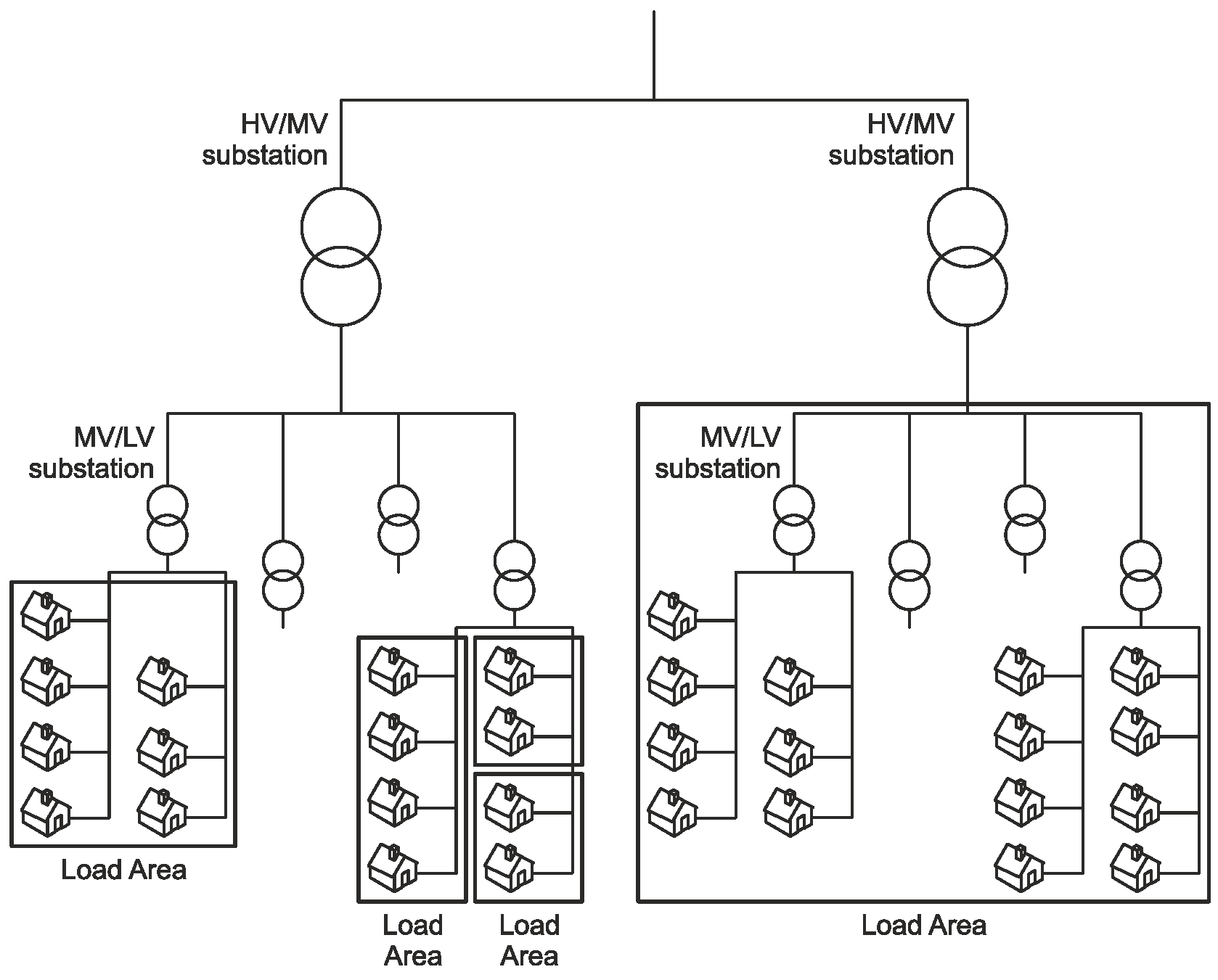
2. Load Area—Concept

The exploitation of DER flexibility involves two different issues. On the one hand, the larger the aggregated flexibility, the bigger the possibility of DERs to actively participate in the power system markets through the aggregator. On the other hand, DERs are scattered within the grids and their flexibility deployment has to be compliant with the grid secure operation. To combine the two needs, the requirement arises of having DERs clusters big enough to offer significant flexibility volumes in the market but sufficiently detailed to avoid masking possibly relevant grid issues.
In a distribution network where flexibility is deployed, although the DSO might not be the user of flexibility, it (and possibly also the Transmission System Operator—TSO) has to verify that the flexibility exchanges do not negatively impact the security of the grid operation. On the other hand, the DSO/TSO may be interested in purchasing flexibility for its own needs [22]. To comply with the two-sided role, the control centre of the DSO has to be equipped with new/updated monitoring and control functions [23,24,25]. The information made available in the DSO’s new control centre allows consideration of the distribution network with a high level of detail, possibly down to the individual phases of a bus. However, such information on flexibility provider locations would be uselessly detailed and cumbersome for the management of flexibility by the aggregator and could be unnecessarily detailed even for the DSO. A relevant simplification could be achieved by selecting and treating only the relevant information, with benefits for the aggregator and even for the DSO [26]. In this view, there are proposals to model distribution networks similar to the transmission ones [27] or to group part of the network for monitoring purposes [28].
In the ADDRESS project [4], the LA approach has been proposed for the management of DER flexibility. An LA is the grouping of network nodes of which power injection has a similar impact on the relevant network operating conditions [19]. For the aggregator, the LAs are the perimeters to which the modelling and forecasting of the aggregated flexibilities to present to the market have to be referred, with a representation compliant with the secure grid operation. The DSO identifies LAs and makes available location information of flexibility providers to all interested parties (in particular, to the aggregator); that information should include the individual commercial code, the LA code, and larger load area information tailored according to the security point of view of the TSO [22].
An LA is a way for representing in a compact way clusters of network nodes to which DERs are connected. In this view, it is similar to a Virtual Power Plant (VPP), by which the aggregated DERs behind a transmission node are modeled as if they were a single power plant connected to the node [2,29,30]. In a VPP, the aggregated technical characterization embeds in some way (for example, with an optimal power flow [2]) the electrical subnetwork which connects the DERs; on the contrary, such a network is explicitly taken into account in the LA approach. Moreover, an LA does not have a predefined perimeter: it will be as big as the operating constraints allow, thus helping the aggregation business, and as small as necessary for a correct network security management by the DSO. To summarize, a VPP is a representation of a subnetwork as seen from its point of coupling to the higher voltage grid and an LA is a clustering of nodes within a grid; it has a perimeter dictated by the issues the SO has to consider to ensure a secure grid operation.
Reconfiguration of the grid may influence the LAs’ identification. While the number of possible configurations can be very high, the number of those effectively realized is reduced to a limited number of cases [31] and the need to update the configuration is usually seasonal and can be forecast [32,33]. It is possible to find a limited number of LAs that fits all the configurations actually realized; the reader is referred to Reference [34] for details of the method.
In addition to meeting the needs of aggregation, a simplified network modeling can derive from the LA concept [35,36]. It can support and foster the adoption of recently a proposed method concerning load management in smart grids [37], autonomous yet interacting subnetworks [38], implementation of demand response programs [38,39,40], and reduction of the information burden for the purposes of the DSO [21].

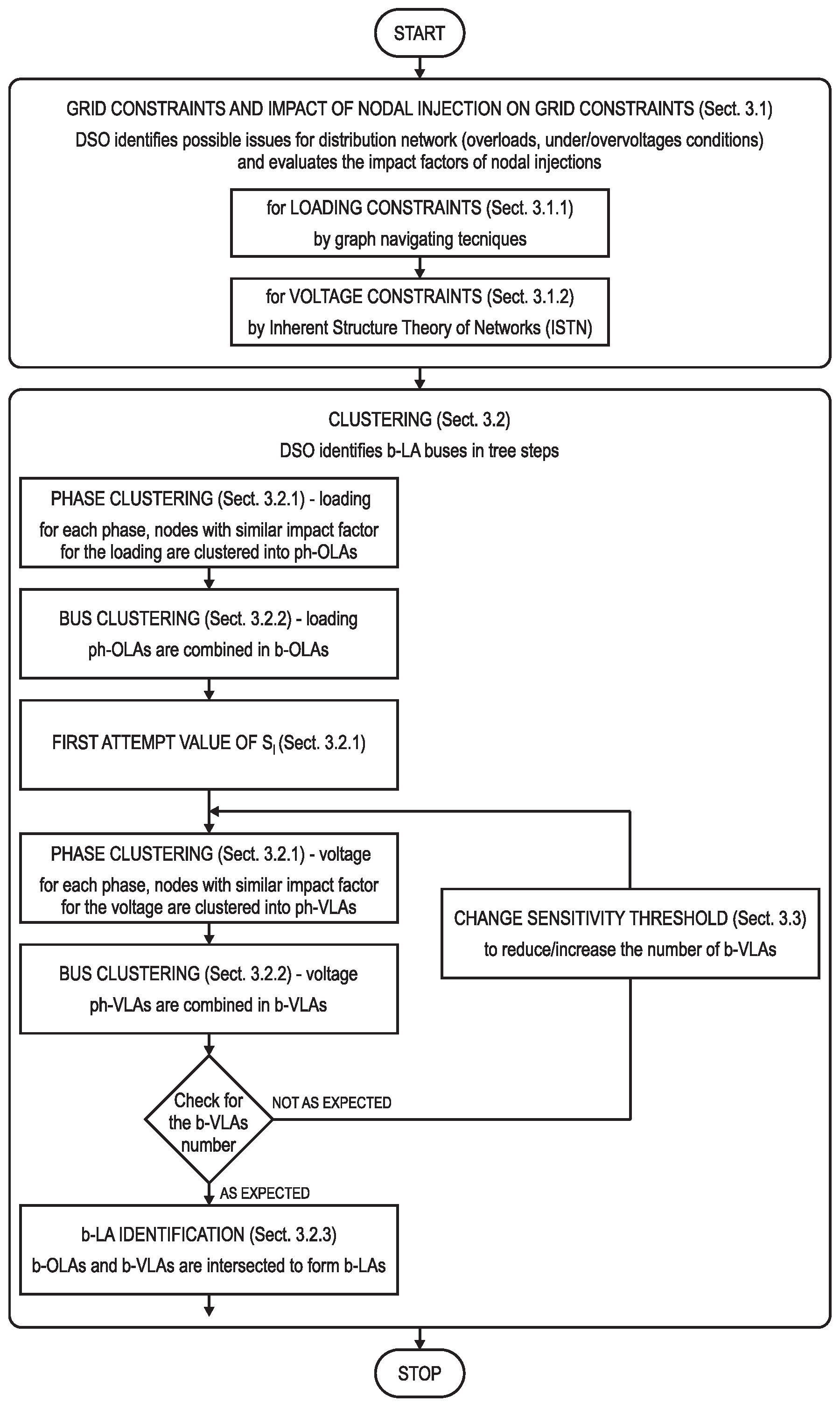
3. Load Area—Identification

According to the definition of LA, a whole distribution system can be seen as a composition of LAs (see Figure 1). Previous papers by the authors have dealt with different issues related to LAs: representation [20], radial equivalent circuit [35], specialized methods for compact representation [36], network reconfiguration [34], and accuracy of the compact modeling [21]; in the aforementioned papers, balanced distribution systems have been considered.
In the case of an unbalanced distribution system, representation with a single phase equivalent is not possible and a three-phase representation is required, which models in detail the spatial geometry of the lines, the connection of the phases and the missing phases, and the unbalanced loads [41].
From a conceptual point of view, the application of the methods already developed for balanced systems to unbalanced ones, represented as three-phase circuits, would result in LAs distinct per phase. However, to keep the aggregator from unnecessary and cumbersome information treatment, it is preferable to have an LA based on busses; it avoids considering the detail of the phases to which the flexibility providers are connected and simplifies their management. Nonetheless, the bus-based LA information has to preserve the phase details of network operating conditions, as required by the DSO.
The method for obtaining bus-based LAs for an unbalanced radial distribution grid is presented in the following, which complies with the combined needs of location information of the aggregator and DSO. The whole procedure is summarized in Figure 2, where the numbers refer to the corresponding sections describing each step.
Since it is necessary to distinguish between phases and busses, which may be single-, or two-, or three-phase, in the subsequent paragraphs, the terminology of [42] is adopted: the term “node” is used to refer to a single phase in a bus, while a “bus” is a group of nodes in the same location and may consist of one to three nodes.

3.1. Grid Constraints and Impact of Nodal Injections

According to well-known security procedures, DSO identifies possible incorrect operations (overload, under/overvoltage) on the basis of historical data collected in the Distribution Management System, possibly in conjunction with load flow analysis.
The impact of each nodal injection is evaluated separately for the identified loading constraints and for the overall voltage profile.

3.1.1. Loading Constraints

For each overload operating condition, in a radial network, the list of all the nodes downstream of the involved component is built with simple graph navigating techniques; the impact of a nodal injection on the given overload condition is set to one if it is in the list and to zero otherwise.

3.1.2. Voltage Constraints

The impact of each nodal injection on the voltages can be evaluated in a comprehensive way in the framework of the Inherent Structure Theory of Networks—ISTN [19,20,43,44,45]; accordingly, the impact of a nodal injection on any nodal voltage is evaluated by its influence on the voltage dominating components.
As well-known, nodal voltages, U ¯ , and currents injected in the nodes, J ¯ , are related by the following (matrix-vector notation applies):
J ¯ = Y ˙ U ¯ ,
where Y ˙ is the three-phase n × n nodal admittance matrix, n is the number of nodes [46,47]; and matrix Y ˙ can be expressed as follows:
Y ˙ = Λ ˙ D λ ˙ t Λ ˙ 1 ,
with λ ˙ representing the n-vector of the eigenvalues of Y ˙ ( λ ˙ t is its tth component), Λ ˙ is an n × n matrix of which the columns are the corresponding eigenvectors (assumed to be independent from each other), and D { x t } represents the diagonal matrix of which the elements along the principal diagonal are the components of vector x.
If no eigenvalue is zero, the L 2 -norm of the node voltage vector can be expressed as follows:
| | U ¯ | | = | | Y ˙ 1 J ¯ | | = | | t = 1 n 1 λ ˙ t S ˙ t J ¯ | | | | t T 1 λ ˙ t S ˙ t J ¯ | | ,
where S ˙ t is the tth eigenvalue sensitivity matrix,
S ˙ t = λ ˙ t Y ˙ 11 λ ˙ t Y ˙ 1 n λ ˙ t Y ˙ n 1 λ ˙ t Y n n ,
and T represents the subset of eigenvalues with minimum modulus of appropriate cardinality. For sensitivity analysis, in a single-phase representation, the acceptable cardinality of T is typically equal to one [20,43,44,45]; in a three-phase representation, we can expect that such minimum cardinality is equal to three, as confirmed by numerical experiments (see Appendix A).
Each matrix element in Equation (4) represents the sensitivity of the tth eigenvalue to the corresponding element of the nodal admittance matrix [43]. A variation of the injection at the generic ith node is seen as a variation of (only) the ith self-admittance element, Y ˙ i , i ; thus, the ith diagonal element of matrix S ˙ t in Equation (4), S ˙ t ( i , i ) , represents the sensitivity of the tth eigenvalue, λ ˙ t , to the variation of injection at the ith node.
For the ith node, the quantity S r ( i ) is as follows:
S r ( i ) = | | t T 1 λ ˙ t S ˙ t ( i , i ) | | / max j | | t T 1 λ ˙ t S ˙ t ( j , j ) | | ;
it is the normalized impact of the variation of the injection at that node on the most significant components of the nodal voltages, which are related to the dominant spectral components of the admittance matrix. As such, it measures the impact of the variation of the injection at the ith node on the nodal voltages. The normalized sensitivity S r ( i ) in Equation (5) is a modification of the analogous quantity for balanced systems proposed in Reference [19,20]: by the summation over T, it accounts for c a r d { T } > 1 , while the multiplication by 1 / λ ˙ t accounts for the relative impact of the most significant eigenvalues.
Therefore, if voltage constraints are of concern for the security of the operation, nodes can be clustered based on the S r , intended as a score of the sensitivity of the voltage profile to nodal injections.

3.2. Clustering

The node/bus clustering into LAs for unbalanced systems consists of three steps. The illustration of the steps is carried out with reference to the network of Figure 3, taken as a working example; in the figure, the three phases are generically indicated as 1, 2, and 3 and evidenced by different colors. Nodes are depicted as black dots, while busses are rounded rectangle encircling nodes, e.g., bus 611 is single-phase, bus 645 is two-phase, and bus 633 is three-phase.

3.2.1. Phase Clustering

For each phase independent from the others, the nodes with comparable values of impact factors for the loading and voltage issues are clustered together into phase Overload Load Areas (ph-OLAs) and phase Voltage Load Areas (ph-VLAs), respectively, as follows.
Loading—For each phase and each loading constraint, the nodes with a unitary impact factor for that constraint are clustered in a ph-OLA.
Voltage—For each phase, nodes are ordered based on the value of S r ( i ) in Equation (5) [19,20]; two consecutive nodes in this ordering, h and k, are considered to belong to different ph-VLAs if
| S r ( h ) S r ( k ) | > S l ,
where S l is a given threshold.
Previous papers by the authors have dealt with LAs in balanced grids modeled as single-phase grids [20,21,34,35,36]. The main difference with the method presented here regards the identification of VLAs, which relies on the spectral representation of the bus-admittance matrix. A comparison of the spectral analysis of admittance matrices for single-phase and three-phase representations is presented in Appendix A. From those results, some considerations can be derived for VLAs:
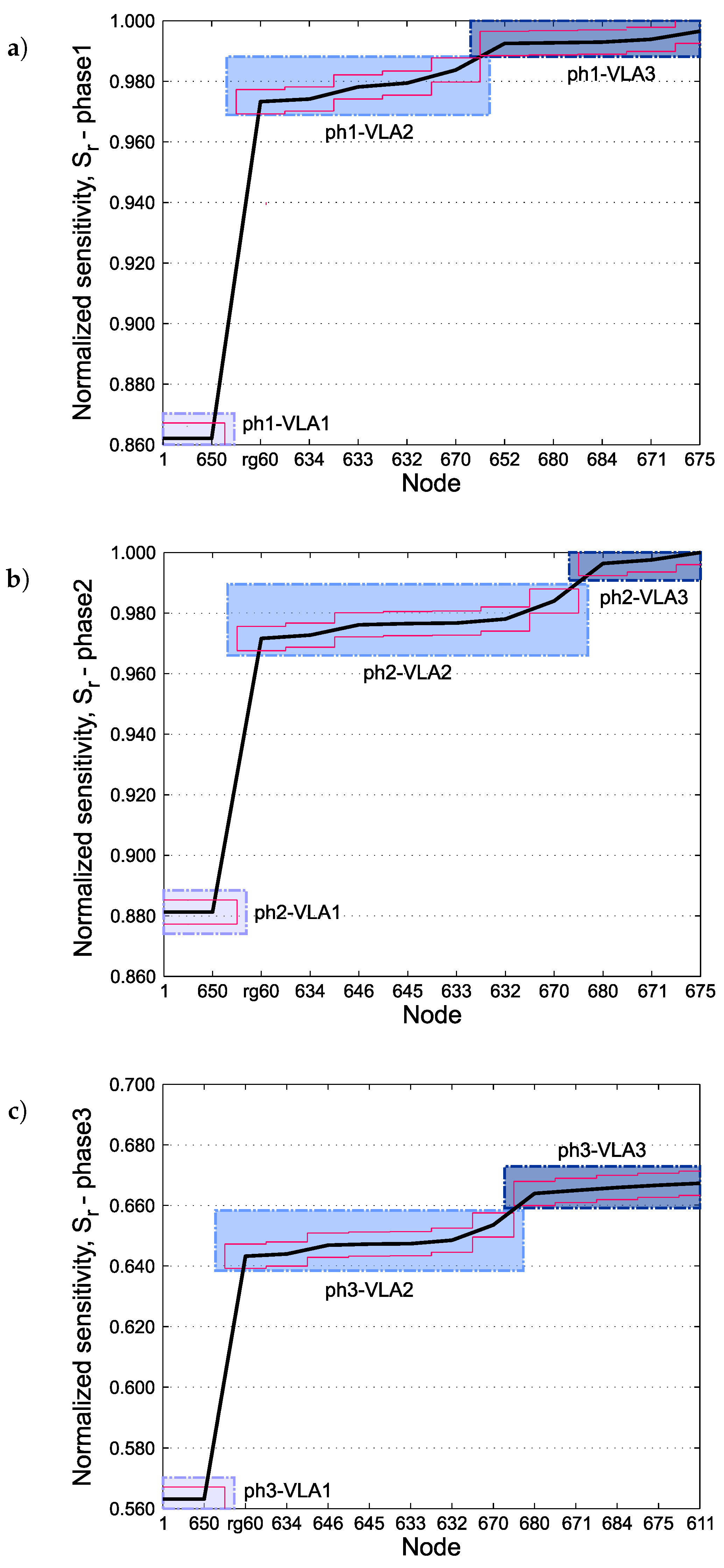
  • The VLAs resulting from a single-phase representation of the grid (the positive sequence grid) are valid within the hypotheses behind the single-phase equivalencing: a grid made of physically symmetrical three-phase components operating in balanced conditions;
  • If any of the two assumptions is not valid, VLAs obtained with a single-phase representation of the grid are only approximated and better results are obtained with the three-phase representation.
The result of the phase clustering step is evidenced in Figure 4 for ph-VLAs; a bold coloured stripe for each phase depicts a ph-VLA, and a white space along a stripe represents a border of a ph-VLA. Similar results are obtained for ph-OLAs.

3.2.2. Bus Clustering
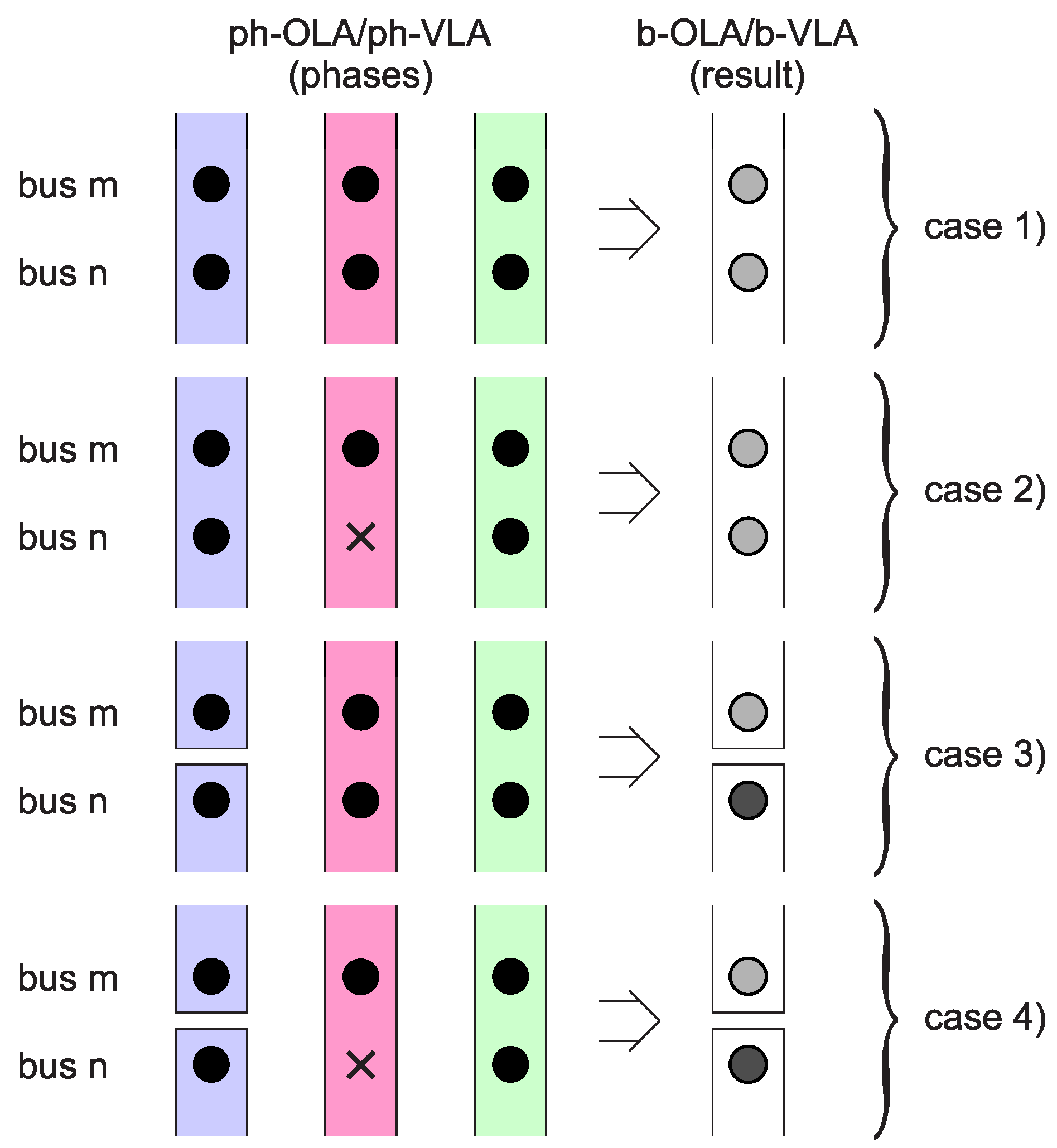
The phase clusters are combined to get bus-based clusters; this phase allows for defining bus Overload Load Areas (b-OLAs) and bus Voltage Load Areas (b-VLAs).
It can be recognized that four possible cases may arise, as summarized in Figure 5, that applies to ph-OLAs or ph-VLAs. In the figure, m and n are two subsequent busses in the radial network, a black circle represents a phase present in a bus while a cross denotes a missing phase, a grey circle indicates the corresponding bus, and the perimeter of a cluster (both phase and bus) is evidenced by a solid line. The fourth column depicts the results of combining the phase clusters into bus-based clusters.
The four possible cases summarized in Figure 5 are as follows:
case 1)
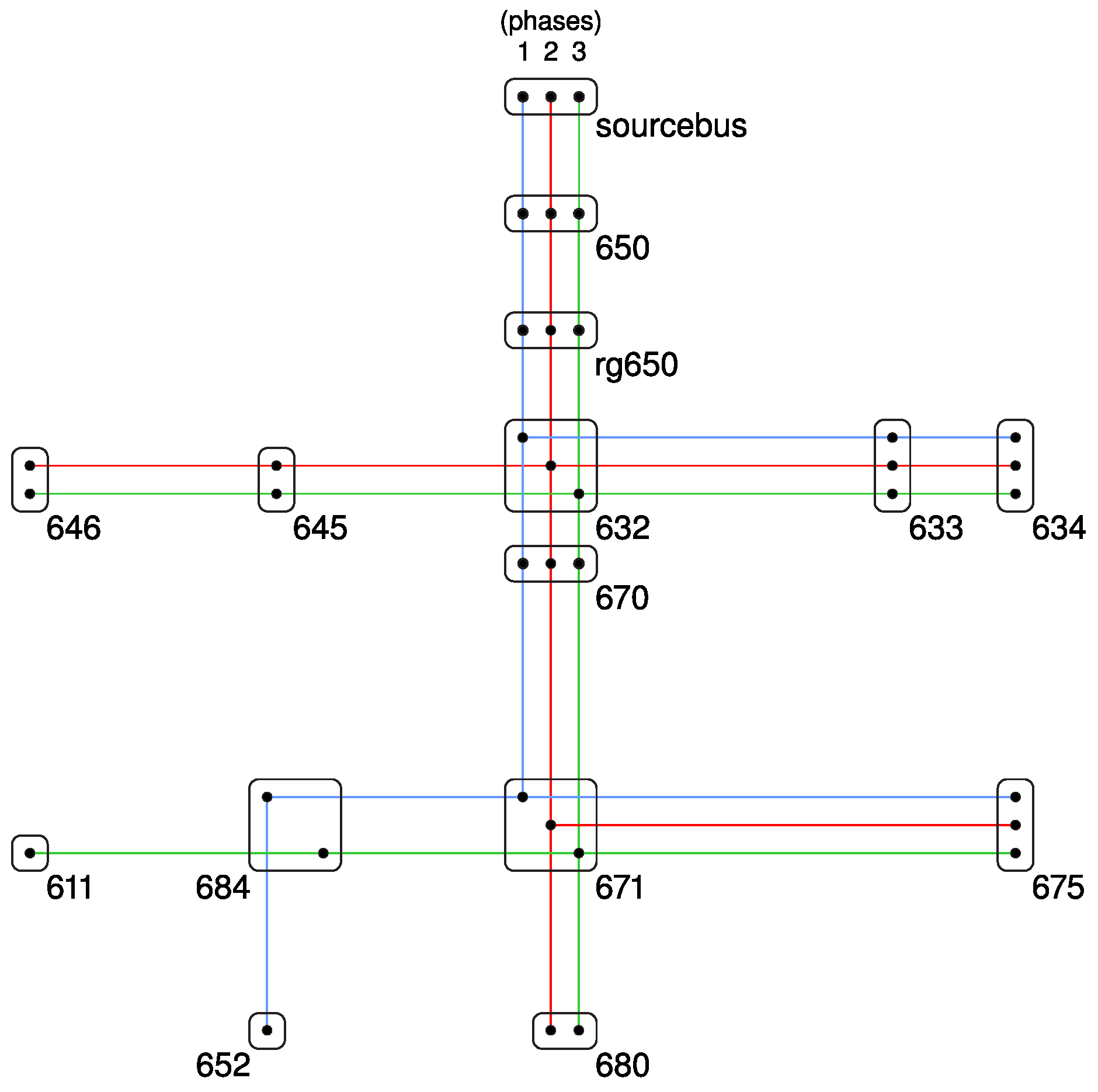
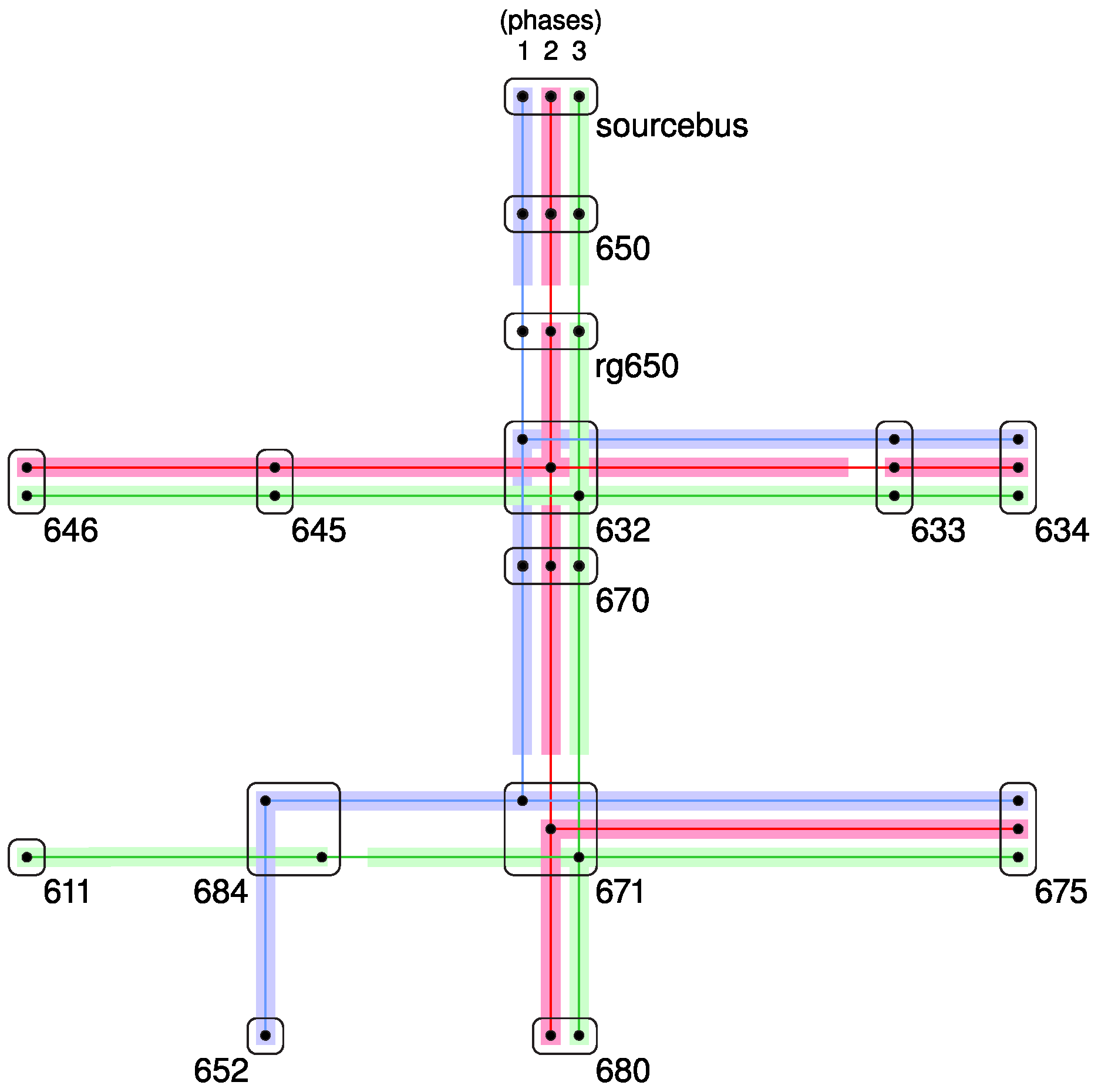
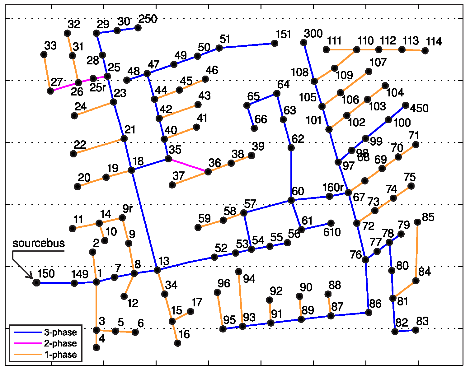
No bus misses any phases, and any phase of a bus belongs to the same ph-OLA/VLA; it is simply reflected in the resulting bus-based LA. This is the case of all the phases showing the same behaviour with respect to overload and voltage issues; for example, in Figure 4, it occurs for sourcebus and bus 650.
case 2)
There is at least one missing phase, and any phase of a bus belongs to the same ph-OLA/VLA; the same bus-based LA as case 1 results. It works as if, for the missing phase, the ph-OLA/VLA is virtually extended downstream from bus m to bus n. This is the case when all the phases would present the same behaviour, but there is at least one missing phase; for example, in Figure 4, it occurs with busses 632 and 645, where the missing phase is phase 1.
case 3)
One or more phases belong to different ph-OLAs/VLAs, and no bus misses any phases. It reflects two different bus-based LAs. This is the case when not all the phases show the same behaviour; for example, in Figure 4, it occurs with busses 632 and 633, where phase 2 shows a different behaviour.
case 4)
There is at least one missing phase, and one or more phases belong to different ph-OLAs/VLAs. The same bus-based LAs as case 3) results. It works as if, for the missing phase(s), the ph-LA is virtually extended downstream from bus m to bus n. This is the case when not all the phases show the same behaviour and there is at least a missing phase; for example, in Figure 4, it occurs with bus 671 and 684, where phase 2 is missing and phase 3 behaves differently in busses m and n.
From the ph-VLAs of Figure 4, the b-VLAs shown in Figure 6 result; it is apparent that the borders of the ph-VLAs determine the borders of the b-VLAs. Once again, similar results are obtained for b-OLAs.

3.2.3. Bus LA

The b-OLAs and the b-VLAs are finally intersected to obtain the b-LAs so that all the busses of the distribution system belong to a b-LA and each bus belongs to only one b-LA [19,20]—see Figure 7. Each b-LA is made of the busses thus obtained and of the lines connecting them; the lines connecting busses belonging to different b-LAs are assumed to belong to the upstream b-LA.

3.3. Choice of the Sensitivity Threshold

The value of the threshold S l in Equation (6) determines the number of ph-VLA and then of the b-VLAs; it is apparent that the lower the value of S l , the higher the number of b-VLAs, and viceversa. A criterion for choosing the value of S l is presented in the following.
From a general point of view, the clustering of nodes into ph-VLAs is a data clustering method; in these methods, sets made of points close to each other with respect to the measure of some characteristic are sought. In data and other clustering problems, there is some degree of arbitrariness [48] and common sense is required to get significant results. Examples of such issue are the methods for defining the architecture of the secondary voltage regulation in transmission systems, in particular the control zones [49,50]; their identification consists in a clustering of nodes based on sensitivities and thresholds, as much as in the method presented in this paper. Based on thresholds, control zones are obtained, and the result has to be supplemented with engineers’ know-how [51].
It is concluded that any clear-cut method for choosing the value of S l cannot be proposed. To define a “common sense” method, it can be observed that the plots of index S i ( r ) (5) usually show significant gaps (see Section 5), which allow ascertaining the number of clusters. A tentative value for S l is set; after the b-VLAs have been obtained, their number is compared to the estimate. If the comparison is not satisfying, the value of S l is changed and new ph-VLAs/b-VLAs are obtained, repeating the process until the comparison is satisfying.

4. Load Area—Modeling

A method for obtaining the compact modeling of a single b-LA is presented, based on the Gaussian elimination. It is a general method; in a radial network, specialized methods could also be exploited [36]. The method presented here is a modification of the general method described in Reference [20,35] and is intended to treat three-phase unbalanced systems.

4.1. Prosumers

In a given geographical area, prosumers can be grouped in categories based on their characteristics: residential, small commercial, distributed generation, etc. [52].
Within a given b-LA, let h represent a prosumer category and k be a prosumer in such category; its active power injection, P h , k , can be considered as a fixed part, p h , k , of the overall active power injection of its category, P h :
P h , k = p h , k P h .
Reactive power injection by the same kth prosumer in the hth category, Q h , k , can be expressed as a function of its active power injection. The general form of this function is as follows:
Q h , k = q h , k f h ( P h ) P h ;
In Appendix B, the expressions of q h , k and f h ( P h ) in Equation (8) are detailed for two prosumer categories.

4.2. Nodal Injections

Let π i _ ϕ , h , k represent the connection of the prosumers to the grid within the given b-LA:
π i _ ϕ , h , k = 1 / ν h , k if the k th prosumer of the h th category is connected in the i th grid bus to the ϕ th phase , and to ν h , k phases in total ; 0 otherwise .
For the ith grid bus, from Equations (7)–(9),
P i _ ϕ i n = h = 1 n c k = 1 n h π i _ ϕ , h , k P h , k = h = 1 n c P h k = 1 n h π i _ ϕ , h , k p h , k = = h = 1 n c π i _ ϕ , h P h , ϕ = 1 , 2 , 3 , Q i _ ϕ i n = h = 1 n c k = 1 n h π i _ ϕ , h , k Q h , k = h = 1 n c f h ( P h ) P h k = 1 n h π i _ ϕ , h , k q h , k = = h = 1 n c ρ i _ ϕ , h f h ( P h ) P h , ϕ = 1 , 2 , 3 ,
where P i _ ϕ i n and Q i _ ϕ i n , ϕ = 1 , 2 , 3 are the active and reactive power injections in each phase, respectively, n c is the number of categories, n h is the number of prosumers in the hth category, and
π i _ ϕ , h = k = 1 n h π i _ ϕ , h , k p h , k , ρ i _ ϕ , h = k = 1 n h π i _ ϕ , h , k q h , k .
From Equations (10) and (11),
J ¯ i _ ϕ p = P i _ ϕ i n j Q i _ ϕ i n U ^ i _ ϕ = 1 U ^ i _ ϕ h = 1 n c π i _ ϕ , h j ρ i _ ϕ , h f h ( P h ) P h ,
where U ¯ i _ ϕ and J ¯ i _ ϕ p are the voltage and the prosumers’ injected current at the ϕ th phase of the ith bus, respectively, and symbol ^ represents the complex conjugate.
For the subsequent development, the value of each voltage is assumed to remain close to that of a reference case, denoted by :
U ¯ i _ ϕ U ¯ i _ ϕ ,
for all busses and all phases. Combining Equations (12) and (13) yields
J ¯ i _ ϕ p 1 U ^ i _ ϕ h = 1 n c π i _ ϕ , h j ρ i _ ϕ , h f h ( P h ) P h = h = 1 n c α ˙ i _ ϕ , h 1 f h ( P h ) P h ,
where
α ˙ i _ ϕ , h = 1 U ^ i _ ϕ π i _ ϕ , h j ρ i _ ϕ , h
is a 1 × 2 matrix.

4.3. Load Area Equivalent Network Modeling

Once a b-LA is identified, the phase voltage at its edge busses and the currents injected there from the outside into the b-LA are easily recognized as relevant quantities to represent the b-LA. In addition, the phase voltage of other, specific busses within the b-LA may be deemed relevant for monitoring and control purposes, for example, the phase voltages of transformers equipped with OLTC. In the following, relevant busses are called describing busses. Let subscript de denote the describing busses and subscript e represent the edge busses (included in de busses); all other busses are denoted by subscript in.
Injected currents are the sum of two contributes: the prosumers’ currents, J ¯ p expressed by Equation (14), and the currents coming from outside the b-LA, J ¯ e x t , which account for the connection of the b-LA to the remainder of the grid. Only for e busses there are external injections, while for all other busses the external injection is zero; recalling that e busses are included in d e busses, it can be written as follows:
J ¯ = J ¯ e x t + J ¯ p = J ¯ e 0 0 + J ¯ p = J ¯ d e 0 + J ¯ p ,
where J ¯ e represents the current injected into the e busses from the outside and the meaning of J ¯ d e is apparent.
From Equations (1), (14), and (16), it is
J ¯ = Y ˙ U ¯ J ¯ d e 0 + h = 1 n c A ˙ d e A ˙ i n h 1 f h ( P h ) P h Y ˙ d e , d e Y ˙ d e , i n Y ˙ i n , d e Y ˙ i n , i n U ¯ d e U ¯ i n ,
where A ˙ . , h is an n L A × 2 matrix of which the rows are the α ˙ i _ ϕ , h in Equation (15) and n L A is the sum of the number of phases in all b-LA busses.
With a Gaussian elimination, an equivalent model of the b-LA based on the d e busses only is obtained from Equation (17):
J ¯ d e = J ¯ e 0 = Y ˙ e q U ¯ d e h = 1 n c Γ ˙ e q , h 1 f h ( P h ) P h ,
where
Y ˙ e q = Y ˙ d e , d e Y ˙ d e , i n Y ˙ i n , i n 1 Y ˙ i n , d e , Γ ˙ e q , h = A ˙ d e , h Y ˙ d e , i n Y ˙ i n , i n 1 A ˙ i n , h ,
with
d i m { Y ˙ e q } = n e q × n e q , d i m { Γ ˙ e q , h } = n e q × 2 ,
and n e q is the sum of the number of phases in all d e busses. Equations (18) and (19) are a description of the b-LA grid based on describing busses and injections by b-LA prosumers.
The second term of the rhs of Equation (18) introduces errors due to Equation (13). For a better approximation, the expression of the prosumers’ equivalent injected currents can be modified and takes into account the phase voltages of d e busses, as in the following:
J ¯ d e = Y ˙ e q U ¯ d e D U ^ d e U ^ d e h = 1 n c Γ ˙ e q , h 1 f h ( P h ) P h .
Approximations still remain due to Equation (13) for the eliminated i n nodes, but the related errors are very low and acceptable from a practical point of view, as observed in Section 5. In terms of powers, Equation (21) represents the usual load-flow equations:
D U ¯ d e J ^ d e = D U ¯ d e Y ^ e q U ^ d e D U ¯ d e D U ¯ d e U ¯ d e h = 1 n c Γ ^ e q , h 1 f h ( P h ) P h = D U ¯ d e Y ^ e q U ^ d e D U ¯ d e h = 1 n c Γ ^ e q , h 1 f h ( P h ) P h ,
with the separate description of the equivalent powers injected by the prosumers (second term of the rhs) and the powers injected through the connections outside the b-LA (lhs).

4.4. Whole Grid Equivalent Network Modeling

Once the compact models of all b-LAs have been obtained, the equivalent model of the whole network can be obtained by connecting these models at their corresponding e busses. The whole network equivalent model would then be made of as many busses as the de busses of all b-LAs but counting only once the same e busses of contiguous b-LAs.
The same equivalent, compact network model of the whole grid could be directly obtained. Based on the results of the b-LA identification, de busses for the whole network can be easily recognized as the ones of the b-LAs (again, recognizing that e busses of contiguous b-LAs have to be counted only once). The injected powers by the prosumers in the whole grid could be expressed as in Equation (14); by applying the modeling procedure of Section 4.3 to the whole network, the equivalent model of the whole grid would be obtained.
The first method should be preferred, since it makes a clear reference to the prosumers within each b-LA, in particular, to the powers injected by each category of prosumers within each b-LA.

5. Study Cases

Two study networks were considered, with pure loads and distributed generation (DG) plants [20]. Grid data were obtained from the IEEE Test feeder [53] and the OpenDSS Simulation Tool [42]. The case of unbalanced three-phase systems is considered; balanced systems are examined in References [20,21,35,54].
b-LAs are identified according to the procedure of Section 3. In all cases, the voltage sensitivity analysis by ISTN (see Section 3.1.2) has been carried out with c a r d { T } = 3 in Equation (5); the addition of the fourth most significant element would only marginally modify the sensitivity results.
Once b-LAs are identified by the DSO; location information of flexibility providers are made public. It comprises the individual commercial code, the b-LA code, and possibly larger LA information. Based on this information, the aggregator is able to propose to the market significant flexibility volumes which are characterized by location from the SOs’ security point of view, in particular, the DSO.

5.1. Small-Size Grid

To illustrate in detail the features of the proposed approach, the b-LA identification and modeling is carried out in detail for the small-size grid of Figure 8, derived from IEEE 13-bus test feeder; the colors evidence the number of phases of each line. The b-OLAs and b-VLAs are obtained according to Section 3.

5.1.1. Identification

b-OLA: assuming an overload on lines 632–645, the identification of all busses involved downstream of the constraint is straightforward; two b-OLAs result as highlighted in Figure 9a.
b-VLA: assuming voltage is of concern, the sensitivity analysis of Equations (4)–(6) is carried out; its results are presented for each phase in Figure 10. By the inspection of the figure, two main gaps can be highlighted, three b-VLAs can be expected, and a first attempt value of S l in Equation (6) equal to 0.008 is chosen.
The value of S l is highlighted by a red band around sensitivities. With Equation (6), phases are clustered into ph-VLAs, highlighted with the same color. The clustering results are summarized in Table 1, in which the ph-VLA identification is indicated both for existent (•) and nonexistent phases (x) (see Section 3.2.2). For example, busses 645 and 646 miss phase 1; they inherit the ph1-VLA (VLA2) of bus 634, the first upstream bus with existent phase 1. Three b-VLAs are recognized, as shown in Figure 9b; it has to be noticed that the voltage behaviour of phases is considered in detail and a compact identification based on busses is obtained.
b-LA: according to Section 3, b-LAs are obtained from the intersection of b-OLAs and b-VLAs; the result is depicted in Figure 9c. The lines 650-rg60, 632–645 and 670–671 belong to the upstream b-LA (b-LA1, b-LA3, and b-LA3, respectively). The proposed procedure preserves the loading and voltage sensitivities of each single phase while identifying bus-based LAs.

5.1.2. Modeling

Based on the results of the identification, the equivalent compact models of the four b-LAs are obtained by taking only edge busses as describing busses and based on a load-flow reference case. From Figure 9c, it is apparent that equivalent compact models of b-LA1 to b-LA4 are made of 2, 1, 3, and 1 busses, respectively. After connecting the corresponding edge busses, the equivalent compact representation of the whole grid is obtained (see Section 4.4), made of four busses as depicted in Figure 9d.
The presence of two prosumers’ categories is considered: pure loads and randomly distributed medium-to-large size DG. For varying values of total load, both with and without DG, load flow computations have been carried out on the whole grid and on the equivalent grid of Figure 9d, with both the LA models of Equation (18) and Equation (21). The difference (in modulus) between the voltage amplitudes of the describing nodes in the whole model and in the compact model is a relevant measure of the error introduced by the equivalent modeling; Figure 11 reports in log scale the maximum of such differences for different values of load. According to Reference [26], the error on the voltage can be deemed acceptable if lower than the one due to the smallest tap changer step of OLTCs in the grid; for a 32-step voltage regulator with a range of 10 % , a one-step tap change corresponds to 0.006250 p.u. In Figure 11, this acceptability limit is indicated by a red dash-dot line. From Figure 11, it is apparent that with Equation (21), the error is very low and always acceptable; on the contrary, the model in Equation (18) presents a much higher error and is not always acceptable.

5.2. Medium-Size Grid

The second case refers to the medium-size grid, derived from the 123-bus IEEE test grid, of which the one-line diagram is depicted in Figure 12, where the parts with different number of phases can be recognized. The details of voltage sensitivity analysis and of the combination of ph-VLAs into b-VLAs are omitted here for the sake of space.

5.2.1. Identification

b-OLA: in this case, two overloads are considered, on lines 23–25 and 97–101; also in this case, the identification of b-OLAs is straightforward, of which the results are highlighted in Figure 13a.
b-VLA: assuming voltage is of concern, the sensitivity analysis of Equations (4)–(6) is carried out. Also for this grid, two main gaps are observed in the plots of index S r ( i ) in Equation (5) (not reported here) and three b-VLA can be expected; a threshold value S l of 0.005 is chosen. The procedure of Section 3.2 results in three b-VLAs (Figure 13b).
b-LA: by intersecting b-OLAs and b-VLAs, the b-LAs depicted in Figure 13c are obtained. The lines 150–149, 78–80, 97–101, and 23–25 belong to the corresponding upstream b-LAs (b-LA1, b-LA2, b-LA2, and b-LA2, respectively).

5.2.2. Modeling

Based on the results of the identification, the equivalent compact models of the four b-LAs are obtained by taking only edge busses as describing busses and based on a load-flow reference case. From Figure 13c, it is apparent that equivalent compact models of b-LA1 to b-LA5 are made of 2, 4, 1, 1, and 1 busses, respectively. After connecting the corresponding edge busses, the equivalent compact representation of the whole grid is obtained (see Section 4.4), made of five busses as depicted in Figure 13d.
As for the small grid, the presence of two prosumers’ categories is considered: pure loads and randomly distributed medium-to-large size DG. The maximum error introduced by the equivalent modelings is reported in log scale in Figure 14. It can be seen that, also for this case, the error with Equation (21) is very low and always acceptable, as highlighted by the limit of 0.00625 represented with a red dash-dot line in Figure 14.

5.3. Some Qualitative Considerations

As illustrated in Section 3.2.1, a grid made of unsymmetrical components or operating in unbalanced conditions requires a three-phase modeling. An accurate comparison between the results of LA identification obtained with single-phase and three-phase representations is then not possible. Nevertheless, some qualitative considerations can be carried out.
By comparing the results of the two study grids with those obtained for the same grids represented as single-phase grids in Reference [20,54], we note the following:
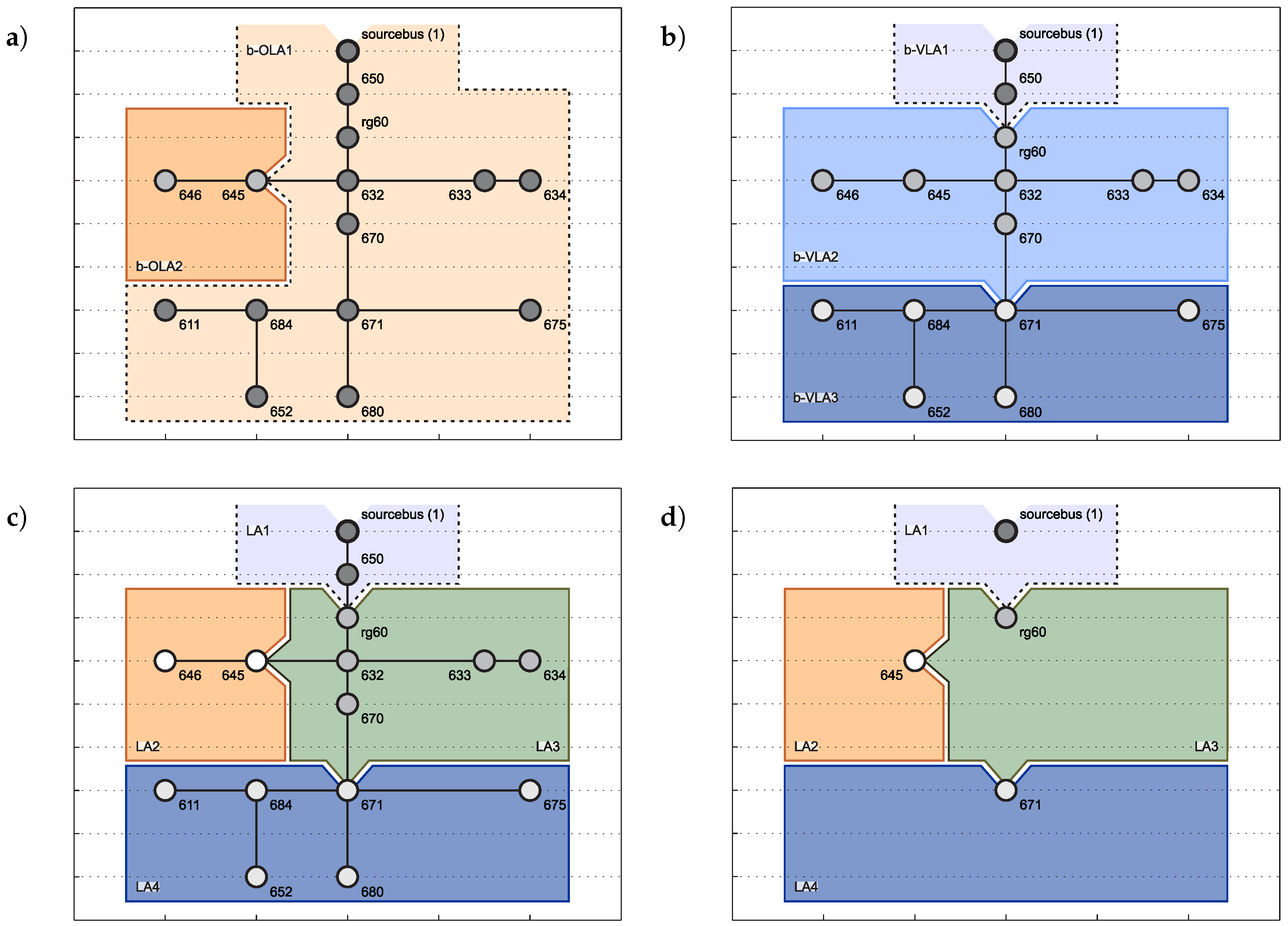
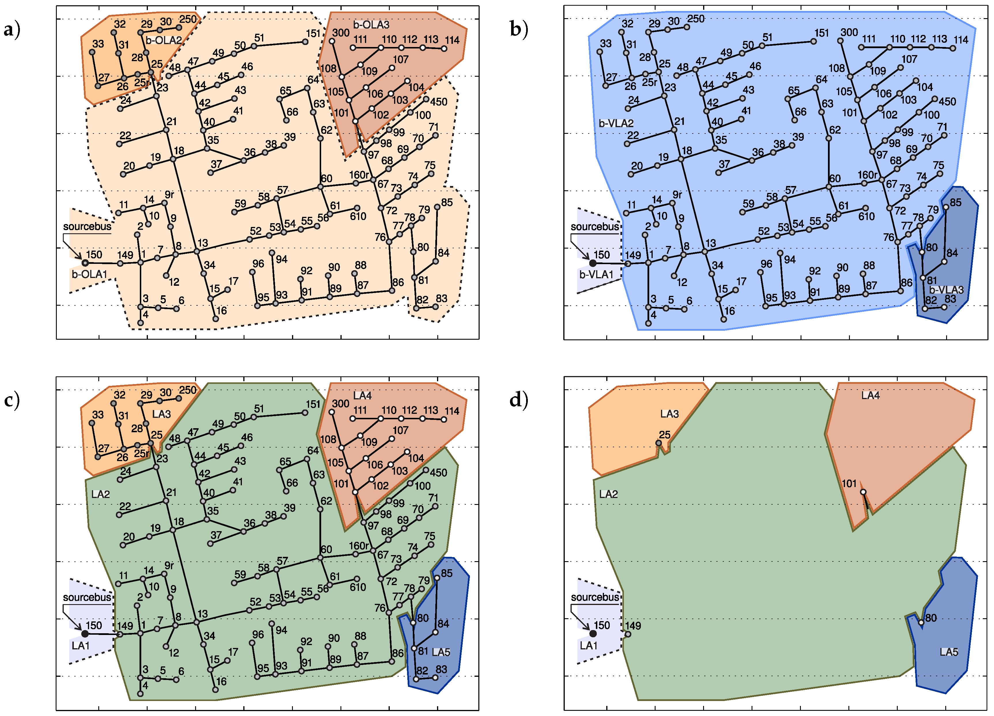
  • The number of identified LAs is almost the same; with the three-phase representation, the number can be slightly bigger (see Figure 5).
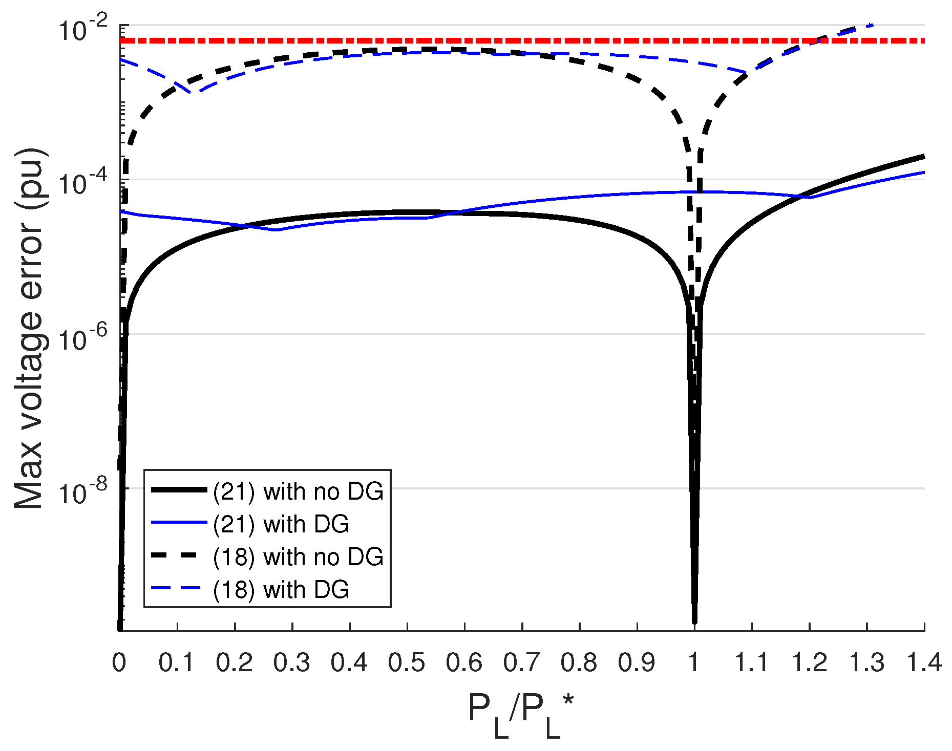
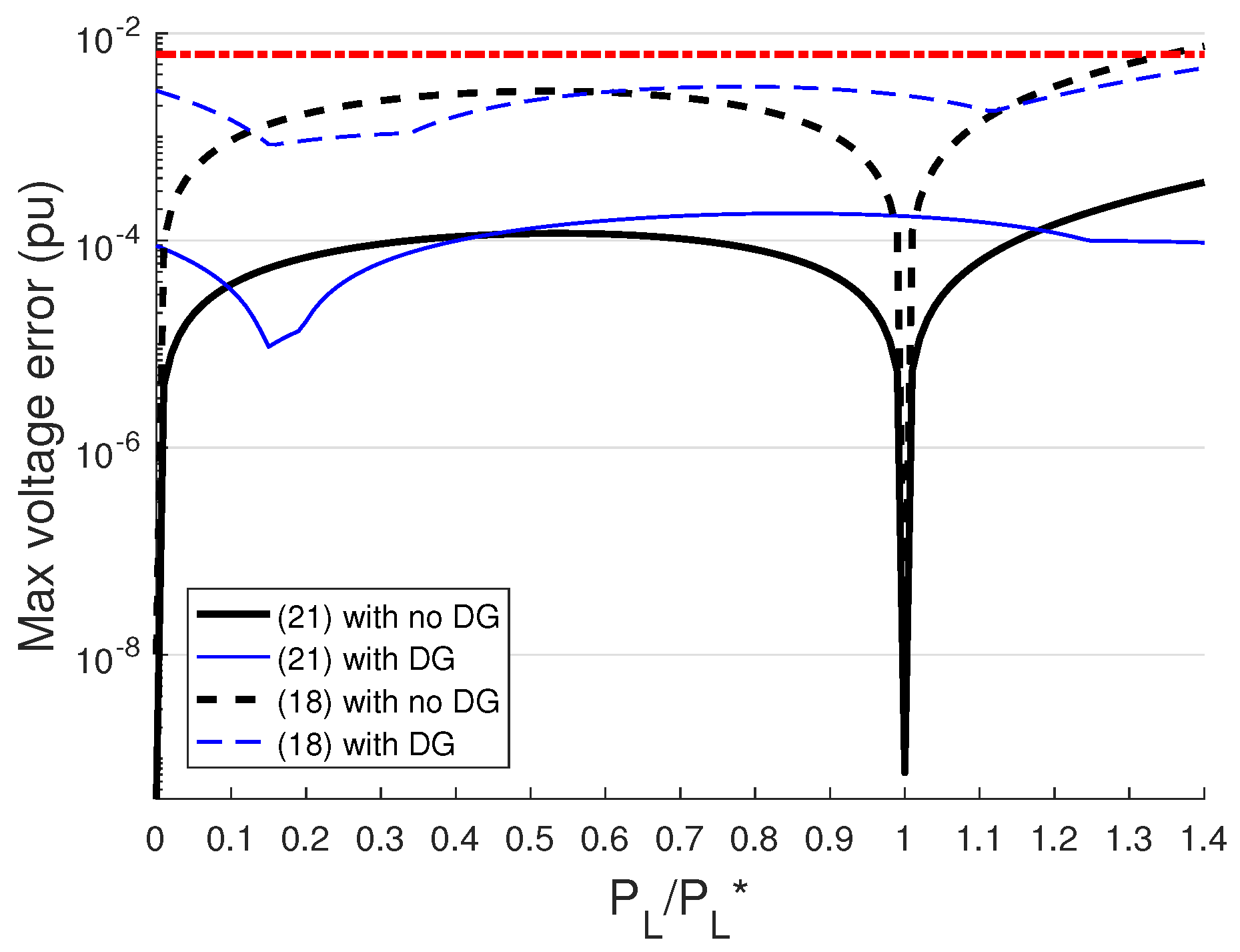
  • The modeling errors are of the same magnitude.
For the sake of space, we do not report here the results obtained for a very big unbalanced grid (almost 4800 busses with 8500 nodes—[53]), analysed as a single-phase grid in Reference [20]. As for the smaller grids, the number of identified LAs with single-phase and three-phase representations is almost the same. The modeling error (for any representation) is higher than that for the smaller grids but always well within the acceptability limit. For very big grids, it can be presumed that unacceptable modeling errors could result; they could be easily reduced by increasing the number of b-LAs (in particular, of b-VLA) through the reduction of the threshold S l in Equation (6).

6. Conclusions

This paper proposes a method to identify and model Load Areas (LAs) of unbalanced three-phase radial networks. The individual characteristics of each phase are taken into account, and bus-based LAs representing the grid are obtained. To this end, the three-phase representation of the grid is adopted, the right number of dominant eigenvalues of the spectral representation of the admittance matrix is assessed with the support of some theoretical results, and a way to obtain bus-based clustering from phase-clustering is proposed.
The method is applied to two unbalanced grids; it is shown in detail how overload and voltage issues drive the identification of bus-based LAs, taking into account phase behaviour. The results of the identification of bus-based LAs show the effectiveness and viability of the approach to get a compact equivalent model of unbalanced grids, with a significative reduction of the describing information. The compact grid models show very small voltage errors.
Future work will deal with the adoption of specialized methods for radial unbalanced grids to obtain the equivalent compact grid model.

Author Contributions

G.M.C. and A.L. contributed equally to all activities leading to this article.

Funding

This research has been supported by the Italian MIUR program ‘Dipartimenti di Eccellenza 2018-2022’.

Conflicts of Interest

The authors declare no conflict of interest.

Appendix A. Spectral Analysis of Admittance Matrices

Appendix A.1. Phase Representation

Let a b-bus three-phase grid made of physically symmetrical components be represented through its three-phase admittance matrix:
J ¯ ϕ = Y ˙ ϕ U ¯ ϕ ,
where J ¯ ϕ and U ¯ ϕ are the 3 b -vectors of bus/phase injected currents and voltages, respectively, and Y ˙ ϕ is the 3 b × 3 b three-phase bus admittance matrix. It is assumed that the numbering of currents and voltages is the obvious one: along busses and for each bus in phase order.
Admittance matrix Y ˙ ϕ in (A1) can be expressed through the corresponding eigensystem, provided that the independent eigenvectors are 3 b :
Y ˙ ϕ = Λ ˙ ϕ D { λ ˙ ϕ } Λ ˙ ϕ 1 ,
where Λ ˙ ϕ represents the 3 b × 3 b matrix, of which the columns are the eigenvectors of Y ˙ ϕ , and λ ˙ ϕ represents its 3 b eigenvalues.

Appendix A.2. Sequence Representations

Let the same n-bus three-phase grid as above be represented through its three single-phase sequence grids:
J ¯ + = Y ˙ + U ¯ + , J ¯ = Y ˙ U ¯ , J ¯ 0 = Y ˙ 0 U ¯ 0 ,
where the meanings and dimensions of J ¯ , Y ˙ , and U ¯ are apparent and subscripts +, −, and 0 refer to the positive, negative, and zero sequence, respectively. Each admittance matrix in Equation (A3) can be expressed through the corresponding eigensystem:
Y ˙ + = Λ ˙ + D { λ ˙ + } Λ ˙ + 1 , Y ˙ = Λ ˙ D { λ ˙ } Λ ˙ 1 , Y ˙ 0 = Λ ˙ 0 D { λ ˙ 0 } Λ ˙ 0 1 ,
provided that the independent eigenvectors for each sequence are b.
Equation (A3) can be rewritten as follows:
J ¯ + J ¯ J ¯ 0 = Y ˙ + 0 0 0 Y ˙ 0 0 0 Y ˙ 0 U ¯ + U ¯ U ¯ 0 .
It can be noticed that, through Equation (A4), the admittance matrix involved in Equation (A5) admits the following eigen-representation:
Y ˙ + 0 0 0 Y ˙ 0 0 0 Y ˙ 0 = Λ ˙ + 0 0 0 Λ ˙ 0 0 0 Λ ˙ 0 D { λ ˙ + } 0 0 0 D { λ ˙ } 0 0 0 D { λ ˙ 0 } Λ ˙ + 1 0 0 0 Λ ˙ 1 0 0 0 Λ ˙ 0 1 .
Reordering —Let injected currents and phase voltages in Equation (A5) be reordered such that the three sequence currents and voltages for each bus are orderly listed next to each other. It can be accomplished through an appropriate permutation matrix, P; from Equation (A5),
P J ¯ + J ¯ J ¯ 0 = P Y ˙ + 0 0 0 Y ˙ 0 0 0 Y ˙ 0 P P U ¯ + U ¯ U ¯ 0 ,
since P P = I . Equation (A7) can be compactly written as follows:
J ¯ s = Y ˙ s U ¯ s ,
where
J ¯ s = P J ¯ + J ¯ J ¯ 0 = J ¯ 1 , + J ¯ 1 , J ¯ 1 , 0 J ¯ b , + J ¯ b , J ¯ b , 0 , U ¯ s = P U ¯ + U ¯ U ¯ 0 = U ¯ 1 , + U ¯ 1 , U ¯ 1 , 0 U ¯ b , + U ¯ b , U ¯ b , 0 , Y ˙ s = P Y ˙ + 0 0 0 Y ˙ 0 0 0 Y ˙ 0 P .
From Equations (A6), (A9), the eigen-representation of Y ˙ s is as follows:
Y ˙ s = P Λ ˙ + 0 0 0 Λ ˙ 0 0 0 Λ ˙ 0 D { λ ˙ + } 0 0 0 D { λ ˙ } 0 0 0 D { λ ˙ 0 } Λ ˙ + 1 0 0 0 Λ ˙ 1 0 0 0 Λ ˙ 0 1 P , = P Λ ˙ + 0 0 0 Λ ˙ 0 0 0 Λ ˙ 0 P P D { λ ˙ + } 0 0 0 D { λ ˙ } 0 0 0 D { λ ˙ 0 } P P Λ ˙ + 1 0 0 0 Λ ˙ 1 0 0 0 Λ ˙ 0 1 P .
It can be compactly written as follows:
Y ˙ s = Λ ˙ s D { λ ˙ s } Λ ˙ s 1 ,
with
Λ ˙ s = P Λ ˙ + 0 0 0 Λ ˙ 0 0 0 Λ ˙ 0 P , λ ˙ s = P λ ˙ + λ ˙ λ ˙ 0 .

Appendix A.3. Equivalence

As well-known, injected three-phase currents and voltages in Equation (A1) can be directly expressed through their sequence components:
J ¯ ϕ = Y ˙ ϕ U ¯ ϕ D { T ˙ s } J ¯ s = Y ˙ ϕ D { T ˙ s } U ¯ s ,
where T ˙ s is the 3 × 3 sequence-to-phase transformation matrix, D { T ˙ s } is a 3 b × 3 b block diagonal matrix of which the 3 × 3 blocks along the diagonal are equal to matrix T ˙ s , and J ¯ s and U ¯ s are given in Equations (A9). From Equation (A13),
J ¯ s = D { T ˙ s 1 } Y ˙ ϕ D { T ˙ s } U ¯ s .
By comparing Equations (A8) and (A14), it is apparent that
D { T ˙ s 1 } Y ˙ ϕ D { T ˙ s } = Y ˙ s ,
and then, from Equations (A2), (A11), and (A12):
Λ ˙ ϕ = D { T ˙ s } Λ ˙ s = D { T ˙ s } P Λ ˙ + 0 0 0 Λ ˙ 0 0 0 Λ ˙ 0 P , λ ˙ ϕ = λ ˙ s = P λ ˙ + λ ˙ λ ˙ 0 .
The following general result for bus-admittance matrices of a grid made of physically symmetrical components can be summarized:
(a)
The eigenvectors of the three-phase bus admittance matrix, Y ˙ ϕ , can be obtained from those of Y ˙ + , Y ˙ , and Y ˙ 0 (Equation (A16.1));
(b)
The eigenvalues of Y ˙ ϕ are those of the three one-phase sequence admittance matrices, Y ˙ + , Y ˙ , and Y ˙ 0 (Equation (A16.2));
(c)
If the operation of the grid is always a balanced one, the structural analysis of the grid can be carried out with reference to its one-phase equivalent representation, which is the positive-sequence grid; indeed, voltages and currents have only positive sequence components and the contribution of the negative and zero sequence eigensystems is null;
(d)
If, on the contrary, the operation can be unbalanced, the structural analysis should be carried out on the three-phase representation of the grid or, equivalently, as per points (a) and (b), through the three one-phase sequence representations.

Appendix A.4. Experimental Results

Numerical analysis has been carried out on many grids, made either of physically symmetrical or unsymmetrical components, with wye-wye transformers both neutrals grounded. The following characteristics of the results have been observed (the dominant eigenvalue is the one with minimum modulus):
  • In the symmetrical case:
    -
    As it could be expected, the eigenvalues for the positive and negative sequence are equal to each other and different from the zero sequence ones;
    -
    For any sequence, the modulus of the dominant eigenvalue is much lower that the one of the second best, often by two orders of magnitude;
    -
    The modulus difference between the dominant positive/negative and zero sequence eigenvalues is much less than the modulus difference between these eigenvalues and the second best of any sequence.
  • In the unsymmetrical case (where exact sequence networks cannot be obtained):
    -
    The three dominant eigenvalues differ from each other;
    -
    The modulus differences between the three dominant eigenvalues are much less than the modulus differences between them and the other eigenvalues.

Appendix B. Q–P Relationships

The active power injection by the kth prosumer in the hth category, P h , k , can be expressed in the form of Equation (7), reported here for an easy reference:
P h , k = p h , k P h .
The reactive power injection by the same prosumer, Q h , k , can be expressed as a function of its active power injection; the general form of this function is presented in Equation (8), reported here for an easy reference:
Q h , k = q h , k f h ( P h ) P h .
In the following, the expression for Equation (A18) will be derived for two prosumer categories: pure loads and distributed generation.

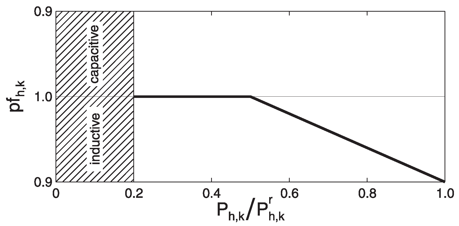
Appendix B.1. Pure Loads

The injection of the kth prosumer in the category category of pure loads can be modeled trough a constant power factor (pf) injection so that
Q h , k = tan φ h , k P h , k , h pure loads ,
with apparent meaning of tan φ h , k . From Equations (A17) and (A19),
Q h , k = tan φ h , k p h , k P h , h pure loads ,
which indicates the dependence of each single reactive power injection (in the pure-loads category) from the active power injection of the whole category.
Equation (A20) can be written as Equation (A18) with
q h , k = tan φ h , k p h , k , f h ( P h ) = 1 , h pure loads .

Appendix B.2. Distributed Generation

Also for DG, the active power injection by the kth plant in the hth DG category can be put in the form of Equation (A17); it means that, in a given region, the DG plants of a given category (for example, PV or wind) generate active power in a similar way. For reactive power, the size of the DG plant has to be taken into account, as in the following.

Appendix B.2.1. Small Plants

Small-size DG plants normally operate at unitary pf [55]. The reactive power injection by the kth DG plant in the small-size-DG category is obtained simply as follows:
Q h , k = 0 , h small DG ,
which can be written in the form of Equation (A18) with
q h , k = n . a . , f h ( P h ) = 0 , h small DG .

Appendix B.2.2. Medium and Large Plants

Medium-to-large-size DG plants are connected to MV or HV distribution systems. It is often required that the reactive power injection of these plants varies depending on the injected active power so that the plants participate to the voltage regulation. DG plants equipped with static converters, for example, should have the pf depicted in Figure A1 [56] and wind DG should have a unitary pf (as the small DG plants) or show a pf-to-P relationship as the one of Figure A1.
Figure A1. Power factor characteristic for medium/large DG plants [20].
Energies 12 03030 g0a1
The pf-to-P dependency of the kth plant in the medium-to-large DG category is expressed versus the per-unit active power injection by the plant (see Figure A1). The rated value of the active power injection by the whole DG category, P h r , is the sum of the rated values of the single plants, P h , k r ; from Equation (7), it follows that
P h , k P h , k r = p h , k P h p h , k P h r = P h P h r .
From Equation (A24),
pf h , k ( P h , k ) = pf h ( P h ) ,
that expresses a pf-to-P relationship valid for the whole DG category. From Equations (A17) and (A25), the reactive power injection by the kth plant in the medium-to-large size DG category can be expressed as follows:
Q h , k = tan arccos ( pf h ( P h ) p h , k P h , h medium to large DG ;
Equation (A26) can be written as Equation (A18) with
q h , k = p h , k , f h ( P h ) = tan arccos ( pf h ( P h ) , h medium to large DG .

References

  1. Sioshansi, F.P. Evolution of Global Electricity Markets: New paradigms, New Challenges, New Approaches, 1st ed.; Academic Press: Cambridge, MA, USA; Elsevier: Amsterdam, The Netherlands, 2013. [Google Scholar]
  2. Pudjianto, D.; Ramsay, C.; Strbac, G. Virtual power plant and system integration of distributed energy resources. IET Renew. Power Gener. 2007, 1, 10–16. [Google Scholar] [CrossRef]
  3. Gottwalt, S.; Garttner, J.; Schmeck, H.; Weinhardt, C. Modeling and valuation of residential demand flexibility for renewable energy integration. IEEE Trans. Smart Grid 2017, 8, 2565–2574. [Google Scholar] [CrossRef]
  4. Belhomme, R.; Cerero Real De Asua, R.; Valtorta, G.; Paice, A.; Bouffard, F.; Rooth, R.; Losi, A. ADDRESS—Active Demand for the smart grids of the future. In Proceedings of the CIRED Seminar 2008: SmartGrids for Distribution, Frankfurt, Germany, 23–24 June 2008; pp. 1–4. [Google Scholar] [CrossRef]
  5. Koponen, P.; Ikäheimo, J.; Vicino, A.; Agnetis, A.; Pascale, G.D.; Ruiz Carames, N.; Jimeno, J.; Sánchez-Úbeda, E.F.; Garcia-Gonzalez, P.; Cossent, R. Toolbox for aggregator of flexible demand. In Proceedings of the 2012 IEEE International Energy Conference and Exhibition (ENERGYCON), Florence, Italy, 9–12 September 2012; pp. 623–628. [Google Scholar] [CrossRef]
  6. De Cerio Mendaza, I.D.; Szczesny, I.G.; Pillai, J.R.; Bak-Jensen, B. Demand response control in low voltage grids for technical and commercial aggregation services. IEEE Trans. Smart Grid 2016, 7, 2771–2780. [Google Scholar] [CrossRef]
  7. Villar, J.; Bessa, R.; Matos, M. Flexibility products and markets: Literature review. Electr. Power Syst. Res. 2018, 154, 329–340. [Google Scholar] [CrossRef]
  8. Asadinejad, A.; Rahimpour, A.; Tomsovic, K.; Qi, H.; Chen, C. Evaluation of residential customer elasticity for incentive based demand response programs. Electr. Power Syst. Res. 2018, 158, 26–36. [Google Scholar] [CrossRef]
  9. Agnetis, A.; Delgado Espinós, I.; Jimeno Huarte, J.; Pranzo, M.; Vicino, A. Active consumer characterization and aggregation. In Integration of Demand Response into the Electricity Chain; Losi, A., Mancarella, P., Vicino, A., Eds.; ISTE: London, UK; Wiley: Hoboken, NJ, USA, 2015; Chapter 2; pp. 11–39. [Google Scholar]
  10. Al-Jassim, Z.; Christoffersen, M.; Wu, Q.; Huang, S.; del Rosario, G.; Corchero, C.; Moreno, M.A. Optimal approach for the interaction between DSOs and aggregators to activate DER flexibility in the distribution grid. CIRED Open Access Proc. J. 2017, 2017, 1912–1916. [Google Scholar] [CrossRef] [Green Version]
  11. Zhang, C.; Wang, Q.; Wang, J.; Pinson, P.; Morales, J.M.; Ostergaard, J. Real-Time Procurement Strategies of a Proactive Distribution Company With Aggregator-Based Demand Response. IEEE Trans. Smart Grid 2018, 9, 766–776. [Google Scholar] [CrossRef]
  12. Lebel, G.; Sandels, C.; Nordström, L.; Grauers, S. Household aggregators development for demand response in Europe. In Proceedings of the 22nd International Conference and Exhibition on Electricity Distribution (CIRED 2013), Stockholm, Sweden, 10–13 June 2013; pp. 1–4. [Google Scholar]
  13. Gkatzikis, L.; Koutsopoulos, I.; Salonidis, T. The role of aggregators in smart grid demand response markets. IEEE J. Sel. Areas Commun. 2013, 31, 1247–1257. [Google Scholar] [CrossRef]
  14. Ruelens, F.; Claessens, B.J.; Vandael, S.; Iacovella, S.; Vingerhoets, P.; Belmans, R. Demand response of a heterogeneous cluster of electric water heaters using batch reinforcement learning. In Proceedings of the 2014 Power Systems Computation Conference, Wroclaw, Poland, 18–22 August 2014; pp. 1–7. [Google Scholar] [CrossRef]
  15. Ruiz, N.; Claessens, B.; Jimeno, J.; López, J.A.; Six, D. Residential load forecasting under a demand response program based on economic incentives. Int. Trans. Electr. Energy Syst. 2015, 25, 1436–1451. [Google Scholar] [CrossRef]
  16. Liu, M.; Shi, Y. Model predictive control of aggregated heterogeneous second-order thermostatically controlled loads for ancillary services. IEEE Trans. Power Syst. 2016, 31, 1963–1971. [Google Scholar] [CrossRef]
  17. Müller, F.L.; Szabo, J.; Sundström, O.; Lygeros, J. Aggregation and disaggregation of energetic flexibility from distributed energy resources. IEEE Trans. Smart Grid 2017, 1205–1214. [Google Scholar] [CrossRef]
  18. Saleh, S.A.; Pijnenburg, P.; Castillo-Guerra, E. Load aggregation from generation-follows-load to load-follows-generation: Residential loads. IEEE Trans. Ind. Appl. 2017, 53, 833–842. [Google Scholar] [CrossRef]
  19. Casolino, G.M.; Fazio, A.R.D.; Losi, A.; Russo, M. Smart modeling and tools for distribution system management and operation. In Proceedings of the 2012 IEEE International Energy Conference and Exhibition (ENERGYCON), Florence, Italy, 9–12 September 2012; pp. 635–640. [Google Scholar] [CrossRef]
  20. Casolino, G.M.; Losi, A. Load areas in distribution systems. In Proceedings of the 2015 IEEE 15th International Conference on Environment and Electrical Engineering (EEEIC), Rome, Italy, 10–13 June 2015; pp. 1637–1642. [Google Scholar] [CrossRef]
  21. Casolino, G.M.; Losi, A. Load Area model accuracy in distribution systems. Electr. Power Syst. Res. 2017, 143, 321–328. [Google Scholar] [CrossRef]
  22. Consiglio, L.; Di Fazio, A.R.; Paoletti, S.; Russo, M.; Timbus, A.; Valtorta, G. Distribution control center: New requirements and functionalities. In Integration of Demand Response into the Electricity Chain; Losi, A., Mancarella, P., Vicino, A., Eds.; ISTE: London, UK; Wiley: Hoboken, NJ, USA, 2015; Chapter 4; pp. 65–87. [Google Scholar]
  23. Valtorta, G.; Consiglio, L.; Morozova, E.; Naso, F.; Narro, J.M.Y.; Vlug, N.; Glorieux, L.; Timbus, A.; Paoletti, S. Medium voltage network control centre functionalities to enable and exploit active demand. In Proceedings of the 2012 IEEE International Energy Conference and Exhibition (ENERGYCON), Florence, Italy, 9–12 September 2012; pp. 647–651. [Google Scholar] [CrossRef]
  24. Lu, X.; Wang, W.; Ma, J. An empirical study of communication infrastructures towards the smart grid: Design, implementation, and evaluation. IEEE Trans. Smart Grid 2013, 4, 170–183. [Google Scholar] [CrossRef]
  25. Yan, Y.; Qian, Y.; Sharif, H.; Tipper, D. A survey on smart grid communication infrastructures: Motivations, requirements and challenges. IEEE Commun. Surv. Tutor. 2013, 15, 5–20. [Google Scholar] [CrossRef]
  26. Eltantawy, A.; Salama, M. A novel zooming algorithm for distribution load flow analysis for smart grid. IEEE Trans. Smart Grid 2014, 5, 1704–1711. [Google Scholar] [CrossRef]
  27. Schmidt, H.P.; Guaraldo, J.C.; da Mota Lopes, M.; Jardini, J.A. Interchangeable balanced and unbalanced network models for integrated analysis of transmission and distribution systems. IEEE Trans. Power Syst. 2015, 30, 2747–2754. [Google Scholar] [CrossRef]
  28. Hu, F.; Sun, K.; Del Rosso, A.; Farantatos, E.; Bhatt, N. Measurement-based real-time voltage stability monitoring for load areas. IEEE Trans. Power Syst. 2015, 31, 1–12. [Google Scholar] [CrossRef]
  29. Etherden, N.; Vyatkin, V.; Bollen, M.H.J. Virtual power plant for grid services using IEC 61850. IEEE Trans. Ind. Inform. 2016, 12, 437–447. [Google Scholar] [CrossRef]
  30. Mnatsakanyan, A.; Kennedy, S.W. A novel demand Response model with an application for a virtual power plant. IEEE Trans. Smart Grid 2015, 6, 230–237. [Google Scholar] [CrossRef]
  31. Rodriguez, F.; Fernandez, S.; Sanz, I.; Moranchel, M. Distributed approach for SmartGrids reconfiguration based on the OSPF routing protocol. IEEE Trans. Ind. Inform. 2015, 12, 1704–1711. [Google Scholar] [CrossRef]
  32. Di Lembo, G.; Petroni, P.; Noce, C. Reduction of power losses and CO2 emissions: Accurate network data to obtain good performances of DMS systems. In Proceedings of the 20th International Conference and Exhibition on Electricity Distribution (CIRED 2009), Prague, Czech Republic, 8–11 June 2009; pp. 1–4. [Google Scholar]
  33. Sapienza, G.; Noce, C.; Valvo, G. Network Technical Losses Precise Evaluation Using Distribution Management System and Accurate Network Data. In Proceedings of the 23th International Conference and Exhibition on Electricity Distribution (CIRED 2015), Lyon, France, 15–18 June 2015; pp. 1–4. [Google Scholar]
  34. Casolino, G.M.; Losi, A. Load areas in reconfiguration of distribution systems. In Proceedings of the 2016 IEEE PES Innovative Smart Grid Technologies Conference Europe (ISGT-Europe), Ljubljana, Slovenia, 9–12 October 2016; pp. 1–6. [Google Scholar] [CrossRef]
  35. Casolino, G.M.; Losi, A. Load Area Application to Radial Distribution Systems. In Proceedings of the 2015 IEEE 1st International Forum on Research and Technologies for Society and Industry Leveraging a better tomorrow (RTSI), Turin, Italy, 16–18 September 2015; pp. 269–273. [Google Scholar] [CrossRef]
  36. Casolino, G.M.; Losi, A. Specialized methods for the implementation of load areas in radial distribution networks. In Proceedings of the 2016 Power Systems Computation Conference (PSCC), Genova, Italy, 20–24 June 2016; pp. 1–7. [Google Scholar] [CrossRef]
  37. Amini, M.H.; Nabi, B.; Haghifam, M.R. Load management using multi-agent systems in smart distribution network. In Proceedings of the 2013 IEEE Power Energy Society General Meeting, Atlanta, GA, USA, 4–8 August 2013; pp. 1–5. [Google Scholar] [CrossRef]
  38. Lo, C.H.; Ansari, N. Decentralized controls and communications for autonomous distribution networks in smart grid. IEEE Trans. Smart Grid 2013, 4, 66–77. [Google Scholar] [CrossRef]
  39. Kamyab, F.; Amini, M.; Sheykhha, S.; Hasanpour, M.; Jalali, M.M. Demand response program in smart grid using supply function bidding mechanism. IEEE Trans. Smart Grid 2016, 7, 1277–1284. [Google Scholar] [CrossRef]
  40. Losi, A.; Mancarella, P.; Vicino, A. (Eds.) Integration of Demand Response into the Electricity Chain: Challenges, Opportunities and Smart Grid Solutions; ISTE: London, UK; Wiley: Hoboken, NJ, USA, 2015; p. 296. [Google Scholar]
  41. Kersting, W.H. Distribution System Modeling and Analysis; CRC Press: Boca Raton, FL, USA, 2012. [Google Scholar]
  42. EPRI, OpenDSS Simulation Tool. Available online: http://smartgrid.epri.com/SimulationTool.aspx (accessed on 1 August 2019).
  43. Laughton, M.A.; El-Iskandarani, M.A. On the inherent network structure. In Proceedings of the 6th PSCC, Darmstadt, Germany, 21–24 August 1978; pp. 188–196. [Google Scholar]
  44. Laughton, M.A.; El-Iskandarani, M.A. The structure of power network voltage profiles. In Proceedings of the 7th PSCC, Lausanne, Switzerland, 12–17 July 1981; pp. 845–851. [Google Scholar]
  45. Carpinelli, G.; Russo, A.; Russo, M.; Verde, P. Inherent structure theory of networks and power system harmonics. IEE Proc. Generat. Transm. Distribut. 1998, 145, 123–132. [Google Scholar] [CrossRef]
  46. Demirok, E.; Kjaer, S.B.; Sera, D.; Teodorescu, R. Three-phase Unbalanced Load Flow Tool for Distribution Networks. In Proceedings of the 2nd International Workshop on Integration of Solar Power Systems—Energynautics GmbH, Lisbon, Portugal, 12–13 November 2012; pp. 1–9. [Google Scholar]
  47. Kersting, W.H.; Green, R.K. The application of Carson’s equation to the steady-state analysis of distribution feeders. In Proceedings of the 2011 IEEE/PES Power Systems Conference and Exposition, Atlanta, GA, USA, 4–8 August 2011; pp. 1–6. [Google Scholar] [CrossRef]
  48. Fortunato, S. Community detection in graphs. Phys. Rep. 2010, 486, 75–174. [Google Scholar] [CrossRef]
  49. Paul, J.P.; Leost, J.Y.; Tesseron, J.M. Survey of the secondary voltage control in France: Present realization and investigations. IEEE Trans. Power Syst. 1987, 2, 505–511. [Google Scholar] [CrossRef]
  50. Arcidiacono, V.; Corsi, S.; Natale, A.; Raffaelli, C.; Menditto, V. New developments in the application of ENEL transmission system voltage and reactive power automatic control. In Proceedings of the 1990 CIGRE Session; CIGRE: Paris, France, 1990; Volume 38/39-06_1990, pp. 1–7. [Google Scholar]
  51. Lagonotte, P.; Sabonnadiere, J.C.; Leost, J.Y.; Paul, J.P. Structural analysis of the electrical system: application to secondary voltage control in France. IEEE Trans. Power Syst. 1989, 4, 479–486. [Google Scholar] [CrossRef]
  52. Gonzales, R.; Kopponen, P.; Hommelberg, M.; Jimeno, J.; Ruiz, N.; Cossent, R.; Vicino, A.; Agnetis, A.; Binet, A.; Zhang, Y.; et al. D2.1—Algorithms for Aggregators, Customers and for Their Equipment which Enables Active Demand. Technical report; ADDRESS Consortium. 2011. Available online: http://www.addressfp7.org/config/files/ADD-WP2-D2.1-Algorithms%20for%20Aggregator_Ebox.pdf (accessed on 1 August 2019).
  53. IEEE PES Test Feeders. Available online: http://sites.ieee.org/pes-testfeeders/resources/ (accessed on 1 August 2019).
  54. Casolino, G.M.; Losi, A.; Noce, C.; Valtorta, G. Network representation in the presence of demand response. In Integration of Demand Response into the Electricity Chain; Losi, A., Mancarella, P., Vicino, A., Eds.; ISTE: London, UK; Wiley: Hoboken, NJ, USA, 2015; Chapter 5; pp. 89–109. [Google Scholar]
  55. CEI. Italian National Standards CEI 0–21: Reference Technical Rules for the Connection of Active and Passive Users to the LV Electrical Utilities; Italian Electrotechnical Committee (CEI): Milan, Italy, 2019. (In Italian) [Google Scholar]
  56. CEI. Italian National Standards CEI 0–16: Reference Technical Rules for the Connection of Active and Passive Consumers to the HV and MV Electrical Networks of Distribution Company; Italian Electrotechnical Committee (CEI): Milan, Italy, 2019. (In Italian) [Google Scholar]
Figure 1. Possible Load Areas (LAs) in a distribution system [19].
Energies 12 03030 g001
Figure 2. Functional block diagram to obtain b-LAs.
Energies 12 03030 g002
Figure 3. Network example.
Energies 12 03030 g003
Figure 4. Phase Voltage Load Areas (ph-VLAs) with coloured bold stripes (similar results for phase Overload Load Areas (ph-OLAs)).
Energies 12 03030 g004
Figure 5. From phase to bus clusters (either OLAs or VLAs).
Energies 12 03030 g005
Figure 6. b-VLAs resulting from ph-VLAs (similar results for b-OLAs).
Energies 12 03030 g006
Figure 7. Example of b-LAs.
Energies 12 03030 g007
Figure 8. Small-size grid.
Energies 12 03030 g008
Figure 9. Small-size grid—(a) b-OLAs; (b) b-VLAs; (c) b-LAs; and (d) compact representation by b-LAs.
Energies 12 03030 g009
Figure 10. Voltage sensitivity analysis for the small-size grid—(a) phase 1; (b) phase 2; and (c) phase 3.
Energies 12 03030 g010
Figure 11. Small grid voltage error, for both the models of Equation (21) and of Equation (18), with S l = 0.008 .
Energies 12 03030 g011
Figure 12. The 123-bus grid.
Energies 12 03030 g012
Figure 13. The 123-bus grid—(a) b-OLAs; (b) b-VLAs; (c) b-LAs; and (d) compact representation by b-LAs.
Energies 12 03030 g013
Figure 14. The 123-bus grid voltage error for both the models in Equation (21) and Equation (18), with S l = 0.005 .
Energies 12 03030 g014
Table 1. Small grid—VLAs per phase and per bus.
ph1-VLAph2-VLAph3-VLAb-VLA
1(•) VLA1(•) VLA1(•) VLA1VLA1
650(•) VLA1(•) VLA1(•) VLA1VLA1
rg60(•) VLA2(•) VLA2(•) VLA2VLA2
632(•) VLA2(•) VLA2(•) VLA2VLA2
633(•) VLA2(•) VLA2(•) VLA2VLA2
634(•) VLA2(•) VLA2(•) VLA2VLA2
645(x) –>VLA2(•) VLA2(•) VLA2VLA2
646(x) –>VLA2(•) VLA2(•) VLA2VLA2
670(•) VLA2(•) VLA2(•) VLA2VLA2
671(•) VLA3(•) VLA3(•) VLA3VLA3
675(•) VLA3(•) VLA3(•) VLA3VLA3
684(•) VLA3(x) –>VLA3(•) VLA3VLA3
680(•) VLA3(•) VLA3(•) VLA3VLA3
652(•) VLA3(x) –>VLA3(x) –>VLA3VLA3
611(x) –>VLA3(•) VLA3(•) VLA3VLA3

