The Uncertain Bidder Pays Principle and Its Implementation in a Simple Integrated Portfolio-Bidding Energy-Reserve Market Model

Abstract

One reason for the allocation of reserves in electricity markets is the uncertainty of demand and supply. If the bias of the generation portfolio shifts from controllable generators to renewable sources with significantly higher uncertainty, it is natural to assume that more reserve has to be allocated. The price of reserve allocation in European models is dominantly paid by the independent system operator in the form of long-term paid reserve capacities and reserve demand bids submitted to various reserve markets. However, if we consider a scenario where the significant part of generation is allocated in day-ahead auctions, the power mix is not known in advance, so the required reserves can not be efficiently curtailed for the ratio of renewables. In the current paper we analyze an integrated European-type, portfolio-bidding energy-reserve market model, which aims to (at least partially) put the burden of reserve allocation costs to the uncertain energy bidders who are partially responsible for the amount of reserves needed. The proposed method in addition proposes a more dynamic and adaptive reserve curtailment method compared to the current practice, while it is formulated in a computationally efficient way.

1. Introduction

Although modern renewable generators do have improved controllability properties compared to earlier solutions, they still exhibit a higher level of supply uncertainty compared to non-renewable generators. In addition, uncertainty is present in several forms in the power grid. First of all, in addition to renewable sources with fundamental characteristics of production uncertainty (of some level), conventional power plants are also naturally subject to failures and technological issues, which may limit their output from time to time. Furthermore, significant part of the demand corresponds to domestic consumers, the schedule of whom may be predicted only with limited accuracy [1,2].

As supply-demand imbalance causes frequency shift in the power network, certain forms of ancillary services (or ‘reserves’ to put it shorter) are needed for frequency stability. Activating these reserves in the appropriate time restores power balance and thus network frequency. Ancillary markets [3] are specialized energy-economical platforms, in which commodities connected to ancillary services are traded. Although there is a broad spectrum of ancillary service and reserve types, in this paper we consider reserves used for frequency control. In a typical ancillary market, reserve providers are paid for allocating the required reserves and an additional fee is paid if the reserve is activated as well. According to this, in the current paper (regarding reserves) we consider capacity-allocation payment (and we are not interested if later the reserve is activated or not and do not consider these activation payments).

Reserves may be classified furthermore into non-event and event driven resources. While non-event driven resources are used to compensate production-consumption imbalances, event driven resources are used in reaction to contingencies and power plant or line outages. In the current article we focus on non-event driven resources and their allocation.

As maintaining the frequency stability of the power grid is the responsibility of the system operator (The terminology may differ as the expressions TSO (transmission system operator) and ISO (independent system operator) are also used for this player. In our case, as reserves will be allocated in the integrated power-reserve auction, we will assume that the operator is in charge not only of the transmission system but also of the auction, so we will use ISO.), it is its task to ensure the allocation of the required amount of reserve via long-term contracts or from the ancillary markets. Ensuring the necessary reserves via long term contracts is by nature more inflexible, as the actual power mix resulting from day ahead power exchanges and its uncertainty properties can not be taken into account. Either the system operator takes a conservative (and costly) approach and allocates a high amount of reserves in long term contracts or uses a mix of long term and short term solutions to account for the actual reserve requirements.

Regarding the general issues of reserve allocation, Reference [4] formulates two general questions: How much reserve should be allocated and who should pay for it? The first problem, in addition to the simple approach presented in the same paper [4], has been a subject to several articles. Following the lead idea of Reference [4], namely that reserve should be purchased up to the point where the marginal cost of providing reserve is equal to the marginal value of this reserve, the article [5] considers the customer outage cost to determine the marginal value of reserve. Regarding more recent approaches, motivated by the increasing market share of renewable sources, stochastic unit commitment based reserve procurement procedure for power systems including wind farms is described in Reference [6], while more or less the same problem is approached by a different solution in Reference [7]. Reference [8] contributes to the same topic by applying a chance-constrained optimization to determine the required amounts of reserve capacity. A robust optimization based method of joint determination of day-ahead energy and reserve dispatch is described in Reference [9]. Allocation of reserve-related costs is however not discussed in detail in these articles.

Regarding the allocation of these costs, which is discussed less in the literature, the original paper [4] gives two approaches: In addition to the most simple solution, namely ‘all consumers should pay a share of the cost of reserve on the basis of their consumption’, it also adds that on the other hand ‘the cost of reserve should be shared among the generators on the basis of their contribution to the need for reserve’. It also discusses the possible scenario when generators forward these cost to their consumers. Regarding the allocation of reserve-related balancing and ramping costs, Reference [10] proposes a unit commitment-based approach, applying the principle of pareto-optimality for the problem. Reference [11] aims to distribute the reserve cost among the most appropriate consumers, applying agent-based modelling and simulation approach. A somewhat similar agent-based approach combined with stochastic unit commitment for the reserve cost allocation problem is presented in Reference [12]. The two latter papers both use the concept of demand factors (first defined in Reference [13]) to characterize the reliability level of customers.

In the current article we follow the second principle formulated in Reference [4] and aim to put the burden of reserve allocation costs to market participants whose activity significantly contributes to the need of reserve allocation. In the context of portfolio-bidding markets, the ‘who pays for’ question is typically answered by the principle that the accepted demand bids cover the costs of products, thus we need to introduce any cost-allocation policy in the form of demand bids. This principle can be considered promising as it fits into the official market development plans of the European Union. It is stated in the Clean Energy Package that ‘all market participants shall be responsible for the imbalances they cause in the system’ and this imposition includes variable renewable energy producers [14]. However, the explicit regulation concerns only balancing markets while the more liquid day-ahead trading platform may remain free of uncertainties. This gap could be filled using a model developed in the current article.

In order to facilitate European market development, the created clearing formulation has to be adjusted to the usual European approach. Thus, in contrast to previous results, which analyzed the problem in a unit commitment framework [15], we consider self-scheduling generators and a purely portfolio-bidding market based framework, consisting energy and reserve markets. We define the concept of supplementary reserve demand bids, which ensure that the owner of any uncertain energy bid, in the case of acceptance, will also automatically contribute to the costs of reserve allocation as well. While uncertainty characterization in the majority of previous literature was focussing to either power plants or customers, in the proposed approach we consider the potential uncertainty of both side of the energy market—both uncertain supply and demand energy bids are considered. Furthermore while previous methods use computationally demanding agent based modelling (as References [11,12]) or include quadratic constraints [10] (or their semidefinite relaxation), we formulate the suggested method as a simple mixed integer linear problem (MILP), which can be efficiently solved, for example, via Benders-decomposition [16] and/or the branch-and-bound algorithm [17]. (Both techniques are widely used to solve problems in the power sector [18,19,20].) In addition, the method suggested in the current paper uses a single scalar parameter according to which the set of uncertain/not uncertain energy bids are defined. Decreasing this parameter from a sufficiently large value, the market implementation of the method presented may be introduced to the market incrementally.

For the aim of simplicity and clarity, we introduce the proposed concept assuming a period decoupled market, in which no multiperiod block orders or minimum income condition (MIC) orders are present, thus every period may be dispatched independently of the others. This means that it is enough for us to define the framework for a single period and introduce the concepts in this context. Later, in Section 4, we discuss the principles according to which the proposed concepts may be implemented in markets using multi-period block orders or MIC orders.

2. Materials and Methods

2.1. Uncertainty Quantification

We assume that every bid of the market can be connected to a bidder. We assume that there are K bidders in the energy market. Similar to the approach of demand factors [12,13], we use simple scalar quantities to characterize the uncertainty of market participants. While in the case of the demand factor the characterizing scalar is formulated as the quotient of the expected energy not supplied (EENS) and the current load, we also account for deviations in the positive direction and define two uncertainty measures corresponding respectively to the positive and negative part of the deviation in question. Based on previous bidding and market behavior of the bidder (or if no data present, then based on the applied technology), we assign the uncertainty quantifiers ($u_k^{+}$ and $u_k^{-}$) for each energy-bidder. The previous market behaviour in this case means that we may analyze how many times and how much the bidder deviated from its previously fixed schedule in relative terms (%) in the positive or in the negative direction, weighted by the quantity of the bid in question. Let us denote the expected relative value in the positive direction of bidder k by $u_k^{+}$, while the expected relative value in the negative direction of bidder k by $u_k^{-}$. By nature, both $u_k^{+}$ and $u_k^{-}$ are non-negative quantities.

For example, let us suppose a bidder corresponding to a renewable source with significant uncertainty. If we have for example, a bid/schedule realization history (H) for bidder k (For the indexing of bidders we use the variable k, while j and i are used for the indexing of bids.) as

$$H=\left(\begin{array}{cccccc}50& 70& 100& 80& 65& 65\\ 41& 73& 92& 80& 63& 69\end{array}\right),$$

(1)

Each column of H corresponds to a previous auction, where the bid of the bidder has been accepted. The top element of each column holds the nominal bid quantity, while the bottom row corresponds to the realized schedule. In this particular case we have the following signed relative deviation vector D (in %).

$$\begin{array}{c}\hfill D_i=100\frac{H_{2,i}-H_{1,i}}{H_{1,i}}\to D=\left(\begin{array}{cccccc}-18& 4.29& -8& 0& -3.08& 6.15\end{array}\right)\end{array}$$

(2)

Taking the positive and the negative part of this vector and weighing with the first row of (1), we get the expected values

$$\begin{array}{c}\hfill u_k^{+}=\frac{{\sum }_i\frac{D_i+\left|D_i\right|}{2}{H}_{1,i}}{{\sum }_i{H}_{1,i}}=1.63\%u_k^{-}=\frac{{\sum }_i\frac{D_i-\left|D_i\right|}{2}{H}_{1,i}}{{\sum }_i{H}_{1,i}}=4.42\%\end{array}$$

(3)

for bidder k. Let us define the positive and negative uncertainty upper bounds ${\overline{u}}^{+}$ and ${\overline{u}}^{-}$. Bids belonging to bidders with $u_k^{+}\ge {\overline{u}}^{+}$ and $u_k^{-}<{\overline{u}}^{-}$ will be called positively uncertain (U+) bids, while bids belonging to bidders with $u_k^{+}<{\overline{u}}^{+}$ and $u_k^{-}\ge {\overline{u}}^{-}$ will be called negatively uncertain (U-) bids. Bids belonging to bidders with both $u_k^{+}\ge {\overline{u}}^{+}$ and $u_k^{-}\ge {\overline{u}}^{-}$ will be called bi-uncertain (Ub) bids.

To consider a simple example, if we assume the above bid with $u_k^{+}=1.63\%$, $u_k^{-}=4.42\%$ and ${\overline{u}}^{+}={\overline{u}}^{-}=2\%$, the bid will be considered as a negatively uncertain bid. In contrast, if ${\overline{u}}^{+}={\overline{u}}^{-}=1\%$, the bid will be taken into account as a bi-uncertain bid.

While the above example was demonstrating the case of a supply bid, we apply the same approach for demand bids as well in the proposed framework (domestic consumers may be for example, considered as uncertain demand bidders).

Let us note that uncertainty upper bounds in general may be different in the case of supply and demand bids, however in this paper we will not distinguish between uncertainty bounds of supply and demand bids. As we will see later, we will use these values to account for reserve allocation needed for the coverage of this uncertainty.

2.2. Market Model of the Single Period Case

We consider a basic portfolio bidding scenario, where participants capable of delivering a certain product (energy or reserve in this case) are represented by supply bids, while entities who are ready to pay for it are submitting demand bids. The market clearing aims to balance the supply with the demand in the terms of the traded quantity and the price.

As in the first step we do not consider multi-period block bids, which define interdependencies over time periods, the calculations for each period may be carried out independently. For this reason, to make the notation more simple, in the first step we describe the calculations regarding only a single time period. Later we discuss how the proposed approach may be generalized for multi-period cases including block orders. Regarding the bid format, the two generally used bid types in portfolio-bidding electricity markets are the step bid and the linear bid. In the case of the step bid the price per unit (PPU) of the bid is independent of the acceptance rate, while in the case of linear bid the price depends on the acceptance rate linearly. In other words, while step bids are parametrized by two values (the quantity (q) and the bid PPU), linear bids are parametrized by the quantity, a starting price and a final price. If a linear bid is partially accepted the resulting PPU may be derived as a linear interpolation of the two prices: If for example, the acceptance rate is 0.5, the resulting PPU is the average of the starting price and the final price. In the proposed framework, for the aim of simplicity and computational efficiency, we do not allow linear bids, only step bids.

In the proposed model, there are 3 sub-markets: the energy sub-market and the reserve sub-markets corresponding to positive and negative reserve. The term ‘sub-market’ is used to emphasize that interdependencies between these markets will be defined and thus they have to be cleared together—in this case the ‘market’ is composed of the sub-markets and the sub-markets are not independent entities anymore.

We do not consider fill-or-kill type bids in the market model, in other words partial acceptance is allowed for all energy bids. Regarding energy bids with uncertainty levels below the thresholds ${\overline{u}}^{+}$ and ${\overline{u}}^{-}$, the variable $y_j^{ES}\in [0,1]$ denotes the acceptance variable of j-th energy supply bid, while $y_j^{ED}\in [0,1]$ denotes the acceptance variable of j-th energy demand bid. In the case of uncertain bids, $y_j^{ESU+}\in [0,1]$, $y_j^{ESU-}\in [0,1]$ and $y_j^{ESUb}\in [0,1]$ denote the acceptance variables of energy supply bids with (respectively positive, negative or both) uncertainty, while $y_j^{EDU+}\in [0,1]$, $y_j^{EDU-}\in [0,1]$ and $y_j^{EDUb}\in [0,1]$ denote the acceptance variables of energy demand bids with uncertainty.

As we will see later, these acceptance indicators will be included in variable vector of the problem. In addition to the acceptance indicators, the variable vector will also hold the income variables, logical integer variables used in the formulation of logical constraints and the market clearing prices (MCP) for energy and reserves. Under market clearing prices we mean prices which are compatible with the bid acceptance and balance constraints (see their formulation later). In other words, if the prices are equal to the market clearing prices, such an acceptance configuration of bids is possible (according to the bid acceptance rules), which ensures the balance of supply and reserve in every sub-market.

2.2.1. Supplementary Reserve Demand Bids

We assume that if uncertainty is present in the dispatch, in the spirit of the uncertain bidder pays principle, reserves must be allocated according to the measure of the uncertainty in question. We assume furthermore that these uncertain sources (being typically non-controllable units) are physically unable to provide reserves which could be used to handle the uncertainty implied by them. As we would like to make uncertain sources and consumers (bidders) pay for the implicated allocation of reserves, we assign obligatory reserve bids in the corresponding (positive, negative or both) reserve markets to each bid submitted in the energy sub-market. We call these compulsorily submitted reserve demand bids supplementary reserve demand bids (SRDBs). Both the bid price and bid quantity of these SRDBs are centrally regulated, they are not determined by the bidder. Uncertain energy bids together with the one or two connected SRDB(s) are called orders. As we will see later, the acceptance of the bids composing the order is dependent on the total income of the order, thus SRDBs and the related orders define interdependencies between the sub-markets.

Let us assume that $y_j^{ESUb}$ is acceptance indicator of the energy supply bid of the bi-uncertain bidder k, the quantity of which is denoted by $q_j^{ESUb}$, while $p_j^{ESUb}$ stands for price per unit (PPU) of the bid. In the proposed setup, implied by the bid corresponding to $y_j^{ESUb}$, bidder k also compulsorily submits a positive and a negative reserve demand bid, whose acceptance indicators are denoted by $y_j^{RD+ESUb}$ and $y_j^{RD-ESUb}$ respectively. The upper index in the notation refers to the set of positive/negative reserve demand bids implied by bi-uncertain energy supply bids.

As it is detailed in the following, the proposed concept of supplementary reserve demand bids may be introduced in the market gradually. In the beginning, it is the task of the ISO to allocate reserves and cover the connected costs. Furthermore, it is plausible that the ISO aims to ensure some of the required reserves in the day-ahead reserve markets. According to this consideration, we consider also reserve bids, which are not connected to uncertain energy bids. In the case when SRDBs cover all reserve needs, the model is completely functional without any non-SRDB reserve demand bid. The acceptance indicators of these (non-SRDB) bids are denoted by $y_j^{RS+}$, $y_j^{RD+}$, $y_j^{RS-}$ and $y_j^{RD-}$ in the case of positive reserve supply, positive reserve demand, negative reserve supply and negative reserve demand respectively.

Returning however to SRDBs, we need to consider the following. As positive deviations must be balanced by negative reserve and vice versa, positively uncertain ES bids ($y_j^{ESU+}$) imply negative reserve demand bids denoted by $y_j^{RD-ESU+}$ and negatively uncertain ES bids ($y_j^{ESU-}$) imply positive reserve demand bids denoted by $y_j^{RD+ESU-}$. In principle, the reserve amounts allocated for these demand bids cover the corresponding expected uncertainty, thus we may write

$$\begin{array}{c}{q}_j^{RD+ESUb}=-q_j^{ESUb}{u}_k^{-}{q}_j^{RD-ESUb}=-q_j^{ESUb}{u}_k^{+}\hfill \\ q_j^{RD+ESU-}=-q_j^{ESU-}{u}_k^{-}{q}_j^{RD-ESU+}=-q_j^{ESU+}{u}_k^{+},\hfill \end{array}$$

(4)

We can see in Equation (4) that following the general convention, throughout the paper we use negative sign for the quantities of demand bids.

We also account for uncertainty in the case of energy demand bids—domestic retail electricity suppliers (who submit demand bids in the wholesale market, which is the subject of our study) may have for example, higher uncertainty compared to bidders corresponding to industrial demand. The notation is similar: the bi-uncertain energy demand bid $y_j^{EDUb}$ implies the a positive and a negative reserve demand bids $y_j^{RD+EDUb}$ and $y_j^{RD-EDUb}$.

In our formalism, we consider demand with negative sign, so the row vectors in Equation (1) will be negative. Positive deviations in this case will mean less consumption, which must be balanced by negative reserves and mutatis mutandis. The SRDBs corresponding to demand bids are described by Equation (5).

$$\begin{array}{c}{q}_j^{RD+EDUb}=q_j^{EDUb}{u}_k^{-}{q}_j^{RD-EDUb}=q_j^{EDUb}{u}_k^{+}\hfill \\ q_j^{RD-EDU+}=q_j^{EDU+}{u}_k^{+}{q}_j^{RD+EDU-}=q_j^{EDU-}{u}_k^{-},\hfill \end{array}$$

(5)

We will suppose that the PPUs of these SRDBs are slightly higher compared to the highest PPU of the submitted reserve supply bids for the corresponding period. The difference is denoted by $\epsilon$ and corresponds to the unit of the market (e.g., 1 EUR/MW). The constant $\epsilon$ is introduced to avoid the possible overlap of supply and demand price curves in the case of the reserve sub-markets, which would potentially undermine the uniqueness of the optimal solution. The SRDB prices are formally defined as

$$\begin{array}{c}\hfill p_j^{RD+SRDB}=\underset{i}{max}\left(p_i^{RS+}\right)+\epsilon p_j^{RD-SRDB}=\underset{i}{max}\left(p_i^{RS-}\right)+\epsilon .\end{array}$$

(6)

where $SRDB\in \{EDUb,EDU-\}$ in the case of positive reserve and $SRDB\in \{EDUb,EDU+\}$ in the case of negative reserve.

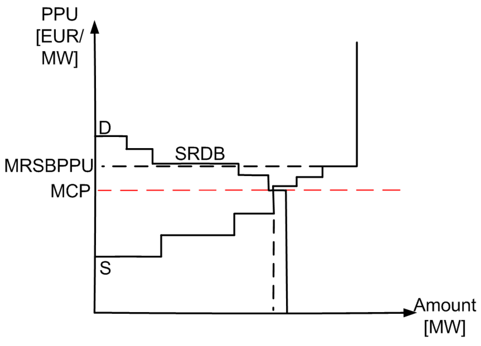
We assume that the amount of reserve supply is always enough to cover the total reserve demand. This assumption is usually valid in practice because regulators enforce power plants to offer reserve services. In this case the bid curves of the reserve spot markets (either positive or negative) will follow the qualitative scheme depicted in Figure 1.

As all SRDBs are accounted for on the price of the supply bid with the highest PPU $+\epsilon$, the central line segment in the demand curve (labeled by SRDB in Figure 1) collects all the SRDBs. The line segments before and after it represent other reserve demand bids submitted to the reserve sub-market.

2.2.2. Minimum Surplus Conditions

Minimum Surplus Conditions for Uncertain Energy Supply Bids

In the proposed setup, without any additional considerations, it is possible that a submitted energy bid is rejected, while the connected SRDB(s) is/are accepted—this would naturally imply loss for the respective order, for the bidder is obliged to pay for the SRDB(s). Furthermore, even if the primary energy bid and the implied SRDB(s) is/are accepted, depending on the resulting MCPs, the surplus from the energy bid (originating from the energy sub-market) may not cover the cost of the SRDB(s) (originating from the reserve sub-markets) or the remaining surplus of the order (after extracting the costs of the SRDBs) may be very small. As the first step in the solution of this problem, we must calculate the incomes of the individual energy/reserve bids.

In order to formulate a linear computational framework, we take advantage of the dependence between MCPs and bid acceptance indicators (y) and use the description of income introduced in References [21,22], as follows. Let us denote the income of the bid corresponding to $y_j^{ESUb}$ by $I_j^{ESUb}$. Intuitively $I_j^{ESUb}$ may be calculated as

$$\begin{array}{c}\hfill I_j^{ESUb}=MC{P}^E{q}_j^{ESUb}{y}_j^{ESUb}\end{array}$$

(7)

where $MC{P}^E$ stands for the market clearing price of energy.

Equation (7) holds however a quadratic expression of variables, namely the product of $MC{P}^E$ and $y_j^{ESUb}$, which would result in a computationally demanding quadratically constrained problem (MIQCP). To overcome this issue we formulate the expressions for income as

$$\begin{array}{c}{y}_j^{ESUb}>0\to I_j^{ESUb}=y_j^{ESUb}{q}_j^{ESUb}{p}_j^{ESUb}+q_j^{ESUb}MC{P}^E-q_j^{ESUb}{p}_j^{ESUb}\hfill \end{array}$$

(8)

$$\begin{array}{c}{y}_j^{ESUb}<1\to I_j^{ESUb}=y_j^{ESUb}{q}_j^{ESUb}{p}_j^{ESUb}\hfill \end{array}$$

(9)

We implement the logical relations in the optimization framework based on the so called big-M method [23], using integer logical variables (denoted by z) as described in Appendix A.

To elucidate the Formulas (8) and (9), let us enumerate the following three possibilities:

• If the bid is entirely accepted ($y_j^{ESUb}=1$), $I_j^{ESUb}$ equals the product of $q_j^{ESUb}$ and $MC{P}^E$ according to (8).
• If the bid is partially accepted ($MC{P}^E=p_j^{ESUb}$), $I_j^{ESUb}$ equals to $y_j^{ESUb}{q}_j^{ESUb}{p}_j^{ESUb}$. Both (8) and (9) are active in this case and they result in the same inequality.
• If the bid is entirely rejected ($y_j^{ESUb}=0$), according to (9) $I_j^{ESUb}=0$.

The above considerations may be naturally formulated also for income of bids corresponding to $y_j^{ESU+}$ and $y_j^{ESU-}$—and also for bids corresponding to $y_j^{ES}$ but their income wont be important in the proposed framework.

The incomes of uncertain energy demand bids $I_j^{EDUb}$, $I_j^{EDU+}$, $I_j^{EDU-}$ and incomes of positive and negative SRDBs connected to energy bids, denoted by, $I_j^{RD+SRDB}$ and $I_j^{RD-SRDB}$ ($SRDB\in \{EDUb,EDU+,EDU-\}$) respectively, may be formulated similarly, taking into consideration in the latter two case that in the case of demand bids $q_j^{RD+SRDB}$ and $q_j^{RD-SRDB}<0$, thus the income will mean practically expense because of the resulting negative sign.

According to these income calculations, now we may formulate constraints which exclude the scenario when the surplus of the primary energy bid does not meet the expense of the SRDB(s). In addition, we assume that for every uncertain order a surplus constant ($S>0$) is defined, which describes how much the surplus of the primary bid must exceed the expenses (in other words it gives a lower bound for the total resulting surplus). In the proposed approach we assume that this constant may be determined by the bidder, thus it is diverse. However, under certain market conditions, it may be also plausible to assume that S is a parameter regulated by the central authority (system/market operator). Regarding the bid corresponding to $y_j^{ESUb}$, we denote this constant by $S_j^{ESUb}$ (the notation is similar in the case of $y_j^{ESU+}$ and $y_j^{ESU-}$). The constant $S_j^{ESUb}>0$, will represent the minimum surplus value, which is required in the case of the acceptance of the order. According to this we may formulate the minimum surplus condition (MSC) for bi-uncertain energy supply bids as

$$\begin{array}{c}\hfill S_j^{ESUb}-I_j^{RD+ESUb}-I_j^{RD-ESUb}\le I_j^{ESUb}-p_j^{ESUb}{q}_j^{ESUb}{y}_j^{ESUb},\end{array}$$

(10)

where the right side is the surplus of the bid and the left side is the sum of the costs of the connected SRDBs (the incomes are negative because of demand) and the parameter $S_j^{ESUb}$. In the case of positively uncertain $ES$ bids, we may write

$$\begin{array}{c}\hfill S_j^{ESU+}-I_j^{RD-ESU+}\le I_j^{ESU+}-p_j^{ESU+}{q}_j^{ESU+}{y}_j^{ESU+},\end{array}$$

(11)

while in the case of negatively uncertain $ES$ bids, the formula becomes

$$\begin{array}{c}\hfill S_j^{ESU-}-I_j^{RD+ESU-}\le I_j^{ESU-}-p_j^{ESU-}{q}_j^{ESU-}{y}_j^{ESU-}.\end{array}$$

(12)

Minimum Surplus Conditions for Uncertain Energy Demand Bids

In the case of bi-uncertain energy demand bids, the minimum surplus condition will state that total cost of the bid must be no more than the maximal potential cost of the bid, which would have been realized in the energy sub-market in the particular case if $MC{P}_i^E=p_j^{ED}$, minus a similar surplus constant ($S_j^{EDUb}$) as in the case of supply bids.

$$\begin{array}{c}\hfill -I_j^{EDUb}-I_j^{RD+EDUb}-I_j^{RD-EDUb}\le -p_j^{EDUb}{q}_j^{EDUb}{y}_j^{EDUb}-S_j^{EDUb},\end{array}$$

(13)

In the case of positively uncertain $ED$ bids, we may write

$$\begin{array}{c}\hfill -I_j^{EDU+}-I_j^{RD-EDU+}\le -p_j^{EDU+}{q}_j^{EDU+}{y}_j^{EDU+}-S_j^{EDU+},\end{array}$$

(14)

while in the case of negatively uncertain $ED$ bids, we may write

$$\begin{array}{c}\hfill -I_j^{EDU-}-I_j^{RD+EDU-}\le -p_j^{EDU-}{q}_j^{EDU-}{y}_j^{EDU-}-S_j^{EDU-}.\end{array}$$

(15)

2.2.3. Bid Acceptance Constraints

For energy supply bids with no uncertainty

• $y_j^{ES}>0\to MC{P}^E\ge p_j^{ES}$.
• $y_j^{ES}<1\to MC{P}^E\le p_j^{ES}$.

For bi-uncertain energy supply bids

• $y_j^{ESUb}>0\to$ Inequality (10) holds. This also implies $MC{P}^E\ge p_j^{ESUb}$.
• $y_j^{ESUb}<1\to MC{P}^E\le p_j^{ESUb}$ or $y_j^{ESUb}=0$, $y_j^{RD+ESUb}=0$ and $y_j^{RD-ESUb}=0$.

For positively uncertain energy supply bids

• $y_j^{ESU+}>0\to$ Inequality (11) holds. This also implies $MC{P}^E\ge p_j^{ESU+}$.
• $y_j^{ESU+}<1\to MC{P}^E\le p_j^{ESU+}$ or $y_j^{ESU+}=0$, and $y_j^{RD-ESU+}=0$.

For negatively uncertain energy supply bids

• $y_j^{ESU-}>0\to$ Inequality (12) holds. This also implies $MC{P}^E\ge p_j^{ESU-}$.
• $y_j^{ESU-}<1\to MC{P}^E\le p_j^{ESU-}$ or $y_j^{ESU-}=0$, and $y_j^{RD+ESU-}=0$.

For energy demand bids with no uncertainty

• $y_j^{ED}>0\to MC{P}^E\le p_j^{ED}$.
• $y_j^{ED}<1\to MC{P}^E\ge p_j^{ED}$.

For bi-uncertain energy demand bids

• $y_j^{EDUb}>0\to$ Inequality (13) holds. This also implies $MC{P}^E\le p_j^{EDUb}$.
• $y_j^{EDUb}<1\to MC{P}^E\ge p_j^{EDUb}$ or $y_j^{EDUb}=0$, $y_j^{RD+EDUb}=0$ and $y_j^{RD-EDUb}=0$.

For positively uncertain energy demand bids

• $y_j^{EDU+}>0\to$ Inequality (14) holds. This also implies $MC{P}^E\le p_j^{EDU+}$.
• $y_j^{EDU+}<1\to MC{P}^E\le p_j^{EDU+}$ or $y_j^{EDU+}=0$, and $y_j^{RD-EDU+}=0$.

For negatively uncertain energy demand bids

• $y_j^{EDU-}>0\to$ Inequality (15) holds. This also implies $MC{P}^E\le p_j^{ESU-}$.
• $y_j^{EDU-}<1\to MC{P}^E\ge p_j^{EDU-}$ or $y_j^{EDU-}=0$, and $y_j^{RD+EDU-}=0$.

For positive reserve supply bids

• $y_j^{RS+}>0\to MC{P}^{R+}\ge p_j^{RS+}$
• $y_j^{RS+}<1\to MC{P}^{R+}\le p_j^{RS+}$

For negative reserve supply bids

• $y_j^{RS-}>0\to MC{P}^{R-}\ge p_j^{RS-}$
• $y_j^{RS-}<1\to MC{P}^{R-}\le p_j^{RS-}$

For not SRDB positive reserve demand bids

• $y_j^{RD+}>0\to MC{P}^{R+}\le p_j^{RD+}$
• $y_j^{RD+}<1\to MC{P}^{R+}\ge p_j^{RD+}$

For not SRDB negative reserve demand bids

• $y_j^{RD-}>0\to MC{P}^{R-}\le p_j^{RD-}$
• $y_j^{RD-}<1\to MC{P}^{R-}\ge p_j^{RD-}$

For positive SRDBs

• $y_j^{RD+SRDB}>0\to$ Inequality (10), (12), (13) or (15) holds (depending on the type of the energy bid in the order of the SRDB) and $MC{P}^{R+}\le p_j^{RD+SRDB}$, where $SRDB\in \{ESUb,ESU-,EDUb,EDU-\}$.
• $y_j^{RD+SRDB}<1\to MC{P}^{R+}\ge p_j^{RD+SRDB}$ or all acceptance indicators of the respective order are 0.

For negative SRDBs

• $y_j^{RD-SRDB}>0\to$ Inequality (10), (11), (13) or (14) holds (depending on the type of the energy bid in the order of the SRDB) and $MC{P}^{R-}\le p_j^{RD-SRDB}$, where $SRDB\in \{ESUb,ESU+,EDUb,EDU+\}$.
• $y_j^{RD-SRDB}<1\to MC{P}^{R-}\ge p_j^{RD-SRDB}$ or all acceptance indicators of the respective order are 0.

The structure of the variable vector and the formulation of logical implications based thereon may be found in Appendix A.

2.2.4. Energy and Reserve Balances

The energy and reserve balances may be formulated as

$$\begin{array}{c}\sum _{j=1}^{n_{ES}}{y}_j^{ES}{q}_j^{ES}+\sum _{j=1}^{n_{ESUb}}{y}_j^{ESUb}{q}_j^{ESUb}+\sum _{j=1}^{n_{ESU+}}{y}_j^{ESU+}{q}_j^{ESU+}+\sum _{j=1}^{n_{ESU-}}{y}_j^{ESU-}{q}_j^{ESU-}\hfill \\ +\sum _{j=1}^{n_{ED}}{y}_j^{ED}{q}_j^{ED}+\sum _{j=1}^{n_{EDUb}}{y}_j^{EDUb}{q}_j^{EDUb}+\sum _{j=1}^{n_{EDU+}}{y}_j^{EDU+}{q}_j^{EDU+}+\sum _{j=1}^{n_{EDU-}}{y}_j^{EDU-}{q}_j^{EDU-}=0,\hfill \end{array}$$

(16)

$$\begin{array}{c}\sum _{j=1}^{n_{RS+}}{y}_j^{RS+}{q}_j^{RS+}+\sum _{j=1}^{n_{RD+}}{y}_j^{RD+}{q}_j^{RD+}+\sum _{j=1}^{n_{ESUb}}{y}_j^{RD+ESUb}{q}_j^{RD+ESUb}+\sum _{j=1}^{n_{EDUb}}{y}_j^{RD+EDUb}{q}_j^{RD+EDUb}\hfill \\ +\sum _{j=1}^{n_{ESU-}}{y}_j^{RD+ESU-}{q}_j^{RD+ESU-}+\sum _{j=1}^{n_{EDU-}}{y}_j^{RD+EDU-}{q}_j^{RD+EDU-}=0,\hfill \end{array}$$

(17)

$$\begin{array}{c}\sum _{j=1}^{n_{RS-}}{y}_j^{RS-}{q}_j^{RS-}+\sum _{j=1}^{n_{RD-}}{y}_j^{RD-}{q}_j^{RD-}+\sum _{j=1}^{n_{ESUb}}{y}_j^{RD-ESUb}{q}_j^{RD-ESUb}+\sum _{j=1}^{n_{EDUb}}{y}_j^{RD-EDUb}{q}_j^{RD-EDUb}\hfill \\ +\sum _{j=1}^{n_{ESU+}}{y}_j^{RD-ESU+}{q}_j^{RD-ESU+}+\sum _{j=1}^{n_{EDU+}}{y}_j^{RD-EDU+}{q}_j^{RD-EDU+}=0.\hfill \end{array}$$

(18)

2.2.5. The Objective Function

The objective function to maximize is the total social welfare (TSW). By definition the TSW is the total utility of consumption minus the total costs of production [24]. The TSW equals in this case the sum of the social welfare in the three sub-markets.

$$\begin{array}{cc}\hfill TSW& =TS{W}^E+TS{W}^{R+}+TS{W}^{R-}\hfill \\ \hfill TS{W}^E& =-\sum _{j=1}^{n_{ES}}{y}_j^{ES}{q}_j^{ES}{p}_j^{ES}-\sum _{j=1}^{n_{ED}}{y}_j^{ED}{q}_j^{ED}{p}_j^{ED}-\sum _{TEU}\sum _{j=1}^{n_{TEU}}{y}_j^{TEU}{q}_j^{TEU}{p}_j^{TEU}\hfill \\ \hfill TS{W}^{R+}& =-\sum _{j=1}^{n_{RS+}}{y}_j^{RS+}{q}_j^{RS+}{p}_j^{RS+}-\sum _{j=1}^{n_{RD+}}{y}_j^{RD+}{q}_j^{RD+}{p}_j^{RD+}\hfill \\ & -\sum _{TEU}\sum _{j=1}^{n_{TEU}}{y}_j^{RD+TEU}{q}_j^{RD+TEU}{p}_j^{RD+TEU}\hfill \\ \hfill TS{W}^{R-}& =-\sum _{j=1}^{n_{RS-}}{y}_j^{RS-}{q}_j^{RS-}{p}_j^{RS-}-\sum _{j=1}^{n_{RD-}}{y}_j^{RD-}{q}_j^{RD-}{p}_j^{RD-}\hfill \\ & -\sum _{TEU}\sum _{j=1}^{n_{TEU}}{y}_j^{RD-TEU}{q}_j^{RD-TEU}{p}_j^{RD-TEU}\hfill \end{array}$$

(19)

where $TEU\in \{ESUb,ESUp,ESUn,EDUb,EDUp,EDUn\}$ denotes set of possible types of uncertain energy bids. Negative signs are needed because of the quantity convention of bids: the amount of demand bids is negative (while supply is positive).

3. Simulation Results

We evaluate the proposed method in the case of a simple, single-period market clearing scenario, where supply and demand bids are submitted to energy and positive and negative reserve markets. SRDBs are created for uncertain energy bids and the market is cleared according to the rules described in Section 2.2. We assume that no network capacities or other limitations constrain the trading (in other words we assume a one-node market). We use the reference bid set described in Appendix B.

As the positive and negative uncertainty upper bounds ${\overline{u}}^{+}$ and ${\overline{u}}^{-}$ define the set of uncertain bids (as described in Section 2.1), decreasing these parameters from a sufficiently large value (which initially implies no uncertain bids) may be viewed also as gradual introduction of the uncertain bidder pays principle to the market. In this section, for the sake of simplicity, we assume that ${\overline{u}}^{+}={\overline{u}}^{-}=\overline{u}$ and analyze the effect of decreasing $\overline{u}$.

3.1. Social Welfare of the Sub-Markets

Figure 2 shows how the TSW values of the energy and reserve sub-markets changes as the parameter $\overline{u}$ is decreased from 30% to 1% in 1% steps. As energy bids with uncertainty values over $\overline{u}$ are considered as uncertain bids, the decrease of this parameter implies an increasing number of uncertain bids. When a bid becomes uncertain, it is submitted with the respective SRDBs and the MSCs come into play. Even if the MCPs do not change, it can happen that, thanks to the newly occurring expenses of SRDBs, a formerly accepted energy bid does not meet the MSC conditions and will be rejected.

Regarding the energy sub-market it can be said that decreasing $\overline{u}$ adds additional constraints to the optimization problem (implied by the SRDBs and corresponding MSCs), thus the decreasing TSW in the first plot of Figure 2 is perfectly plausible.

Regarding the reserve sub-markets, the increase of the TSW depicted in the second plot of Figure 2 may be explained with the increasing number of demand bids. As more and more energy bids are classified as uncertain, more and more SRDBs appear in the markets.

As reserve bids do not correspond to physical production but to the allocation of potential production, usually the bid prices are lower compared to energy bids. This is also reflected in the bid set used for the example and described in Appendix B—the prices of reserve bids are lower. Considering that the volume traded on the reserve markets is also lower, this naturally results in a lesser value of social welfare compared to the energy sub-market.

3.2. Traded Volumes

The traded total volumes in the sub-markets (depicted in Figure 3) show a similar trend to TSWs: As more and more energy bids become uncertain and some of them do not meet the MSCs thus are disregarded. In contrast, with the increasing number of SRDBs, the demand ion the reserve sub-markets is increasing as the parameter $\overline{u}$ is decreased.

3.3. Market Clearing Prices

Regarding the MCPs in different scenarios of the simulation, Figure 4 depicts the results.

The monotone rise in the reserve MCPs depicted in the second plot of Figure 4 may be explained by the increasing demand in the reserve sub-markets: The number of SRDBs, thus reserve demand increases with the number of uncertain energy bids. The effect of this phenomena on the MCP of energy (depicted in the first plot of Figure 4) is however twofold: Here bids become unacceptable due to increasingly occurring MSCs on both the demand and supply side. As the extent of ‘lost’ bids in supply/demand side potentially changes in every step, the change of MCP can not be predicted.

3.4. Computational Properties

As discussed in References [25,26], some of the algorithms used or suggested for electricity market clearing (like EUPHEMIA [17]) contain heuristic elements. In contrast, the proposed model results in a standard MILP problem, which may be approached by any general solver.

To give an impression about the computational requirements and performance of the proposed framework, a small series of computational test were performed. The required computational time was measured as the function of the parameter $\overline{u}$ in the case of 3 different reference bid set containing various numbers of energy bids. The results regarding computational times and number of induced variables are depicted in Figure 5. It can be seen in the figure that as the uncertainty threshold $\overline{u}$ is lowered, with the increasing number of SRDBs, the computational demand shows an increasing trend. The computational demand is dominantly influenced by the number of integer variables, which also increases with the number of SRDBs.

The calculations were performed on a HP Z440 desktop computer, using the IBM CPLEX solver [27] called from MATLAB.

4. Discussion

4.1. Additional Possible Phenomena in the Setup

Figure 6 depicts the TSW of reserve sub-markets in a similar experiment as detailed before and depicted in Figure 2 and Figure 4: The parameter $\overline{u}$ is decreased.

In this figure however, the increase of $TS{W}^{R+}$ is not monotone. The explanation for this is that if for example, an energy bid has a positive uncertainty of 27% and a negative uncertainty of 26%, the following happens. As $\overline{u}$ is decreased to 27%, the bid becomes positively uncertain. If the cost of the implied SRDB is acceptable and the MSC holds, the bid will be still accepted in the energy market and its SRDB will be also accepted, increasing the TSW of the reserve market (compared to the $\overline{u}=28\%$ scenario). However, in the case of $\overline{u}=26\%$, the bid becomes bi-uncertain and instead of one, two SRDBs must be paid for. In this case, it is plausible that the MSC does not hold anymore, resulting in the rejection of all three bids of the order (according to bid acceptance rules). This may be interpreted as a loss of a bid in the positive reserve sub-market, resulting in the decrease of the TSW.

4.2. Total Amount of Allocated Reserve

At a given value of $\overline{u}$, the amount of reserve resulting from the SRDBs is explicitly defined by Equation (4). On the other hand, as discussed before, several principles may be applied to determine the total amount of allocated reserves in the power system [6,7,8,9]. While the advantage of the proposed methodology is that it allocates reserves and the corresponding cost only in the case of accepted uncertain energy bids (due to MSCs) and it is flexible as the current power mix changes, there are no explicit guarantees for the amount of total allocated reserves for the whole system. The total reserve allocated by SRDBs may not meet the thumb rule that stating that the amount of allocated reserve must be at least equal the capacity of the largest unit in service (consider for example, a not-uncertain nuclear power plant and several smaller uncertain renewable sources). This approach is however is generally accepted in the context of event-driven reserves, while, as mentioned earlier, we are focussing on non event-driven resources. The main aim of the proposed approach is not to handle such large and conservative reserve needs (which most of the time may be handled by long term contracts by the system operator) but to provide a framework in which the (hour-level) actual reserve requirements and costs implied by the uncertainties of imminent power mix are automatically allocated.

On the other hand, Equation (4) may be modified by a normalization factor c as described in Equation (20) in order to tune the total amount of allocated reserves.

$$\begin{array}{c}{q}_j^{RD+ESUb}=-q_j^{ESUb}c{u}_k^{-}{q}_j^{RD-ESUb}=-q_j^{ESUb}c{u}_k^{+}\hfill \\ q_j^{RD+ESU-}=-q_j^{ESU-}c{u}_k^{-}{q}_j^{RD-ESU+}=-q_j^{ESU+}c{u}_k^{+},\hfill \end{array}$$

(20)

If the computational capacity is sufficient, this tuning can be carried out via an outer control loop, calculating the dispatch and the total SRDB amount as a function of c. There are no guarantees that any amount of total SRDB-reserves may be allocated with this method (after increasing c above a certain level, none of the MSCs will hold, thus all uncertain bids will be rejected and no SRDB-reserve will be allocated) but this additional parameter may be a useful tool to achieve certain regulation aims.

4.3. Market Implementation

As proposed in Section 3, the values $\overline{u}-$ and $\overline{u}+$ may be decreased step-by-step from high values. During the simulation we analyzed how this decrease affects the various sub-markets assuming the same original bid set.

Regarding the possible market implementation of the method, this decrease of parameters may be carried out on for example, a monthly scale, thus progressively coupling the initially independent energy and reserve sub-markets via the SRDBs and meanwhile giving time for market participants to adapt to the changing regulation.

A further important question arises in connection with widely used special orders in electricity markets. Block orders [28] submitted to the energy sub-market and exhibiting the fill-or-kill property have not been discussed in the current paper for the aim of simplicity. There is no theoretical obstacle however to apply the fundamental principle of the approach for such orders. Considering a multi-period uncertain block order, the respective SRDBs may be defined for each affected period—in this case, the computations for each period must be carried out simultaneously and the income of the block order has to be formulated as the sum of incomes for the different periods. The MSC in this case can be included in the acceptance rules of the block order.

Minimum income condition orders [29], which are basically hourly step orders bound together by the minimum income condition, also define interdependencies between different periods. The novel income formulation of these orders proposed in Reference [21] and also used in this paper can be easily generalized to account also for the expenses of SRDBs, thus the acceptance rules of such bids may be also generalized for the proposed setup.

The proposed formulation is also compatible with general complex orders [22], orders including load gradient conditions (LGC orders) [30] and markets with so called ‘PUN’ orders, where the buyers pay uniform price despite multiple price zones [25].

One must keep in mind however that generalizing the proposed framework for interdependent multi-period clearing mechanisms may be computationally demanding because of the high number of integer variables originating from logical expressions. On the other hand, the MILP framework may be efficiently implemented using novel computational paradigms (e.g., Benders decomposition—see Reference [26]).

5. Conclusions and Future Work

In this article we proposed a method to implement the uncertain bidder pays principle in integrated portfolio-bidding electricity markets, in which the bidders of uncertain energy bids compulsorily submit predefined reserve demand bids (supplementary reserve demand bids or SRDBs) to the reserve markets to account for production/demand uncertainty. The profitability of orders corresponding to uncertain energy bids upon acceptance is ensured in the proposed framework by the minimum surplus conditions (MSC), which bounds the total surplus of the order composed by the uncertain energy bid and the connected SRDBs. As the set of uncertain bids is defined by an uncertainty threshold parameter $\overline{u}$, the proposed framework may be progressively applied, inducing increasing coupling between the initially independent energy and reserve sub-markets. The computational formulation results in a mixed integer linear programming problem (MILP).

Regarding the generalization perspectives of the framework, when we are discussing the implementation of the uncertain bidder pays principle in the context of portfolio-bidding markets, we think that the general question may be formulated as ‘how the uncertainty of a unit/consumer becomes a reserve demand bid, which covers the cost of reserve allocation’. In this paper we proposed an approach which works on the level of single bids. This approach has the benefit that the resulting SRDB (and thus the cost of the reserve) is straightforwardly assigned to a market participant—to the submitter of the uncertain energy bid. A different approach, where the uncertainty of multiple energy bids bids is represented by one reserve demand bid, would allow the more complex handling of uncertainties (e.g., with the possible application of risk measures [31]) but the problem of cost allocation would become more challenging as well. Nevertheless, the general problem of bid/order formulation from uncertain energy bids means a potential research direction for the future, which we plan to pursue based on the current results. A straightforward generalization of the concept is to formulate the approach for multi-period models with the inclusion of block orders and/or minimum income condition (MIC) orders.

References

1. Hernandez, L.; Baladron, C.; Aguiar, J.M.; Carro, B.; Sanchez-Esguevillas, A.J.; Lloret, J.; Massana, J. A survey on electric power demand forecasting: future trends in smart grids, microgrids and smart buildings. IEEE Commun. Surv. Tutor. 2014, 16, 1460–1495. [Google Scholar] [CrossRef]
2. Fallah, S.N.; Ganjkhani, M.; Shamshirband, S.; Chau, K.W. Computational Intelligence on Short-Term Load Forecasting: A Methodological Overview. Energies 2019, 12, 393. [Google Scholar] [CrossRef]
3. Raineri, R.; Rios, S.; Schiele, D. Technical and economic aspects of ancillary services markets in the electric power industry: An international comparison. Energy Policy 2006, 34, 1540–1555. [Google Scholar] [CrossRef]
4. Strbac, G.; Kirschen, D.S. Who should pay for reserve? Electr. J. 2000, 13, 32–37. [Google Scholar] [CrossRef]
5. Afshar, K.; Ehsan, M.; Fotuhi-Firuzabad, M.; Amjady, N. Cost-benefit analysis and MILP for optimal reserve capacity determination in power system. Appl. Math. Comput. 2008, 196, 752–761. [Google Scholar] [CrossRef]
6. Morales, J.M.; Conejo, A.J.; Pérez-Ruiz, J. Economic valuation of reserves in power systems with high penetration of wind power. IEEE Trans. Power Syst. 2009, 24, 900–910. [Google Scholar] [CrossRef]
7. Ortega-Vazquez, M.A.; Kirschen, D.S. Estimating the spinning reserve requirements in systems with significant wind power generation penetration. IEEE Trans. Power Syst. 2008, 24, 114–124. [Google Scholar] [CrossRef]
8. Margellos, K.; Haring, T.; Hokayem, P.; Schubiger, M.; Lygeros, J.; Andersson, G. A robust reserve scheduling technique for power systems with high wind penetration. In Proceedings of the International Conference on Probabilistic Methods Applied to Power Systems, Istanbul, Turkey, 10–14 June 2012. [Google Scholar]
9. Zugno, M.; Conejo, A.J. A robust optimization approach to energy and reserve dispatch in electricity markets. Eur. J. Oper. Res. 2015, 247, 659–671. [Google Scholar] [CrossRef] [Green Version]
10. Haring, T.W.; Kirschen, D.S.; Andersson, G. Efficient allocation of balancing and ramping costs. In Proceedings of the 2014 Power Systems Computation Conference, Wroclaw, Poland, 18–22 August 2014; pp. 1–9. [Google Scholar] [CrossRef]
11. Pinto, T.; Gazafroudi, A.S.; Prieto-Castrillo, F.; Santos, G.; Silva, F.; Corchado, J.M.; Vale, Z. Reserve costs allocation model for energy and reserve market simulation. In Proceedings of the 2017 19th International Conference on Intelligent System Application to Power Systems (ISAP), San Antonio, TX, USA, 17–20 September 2017; pp. 1–6. [Google Scholar]
12. Gazafroudi, A.S.; Shafie-Khah, M.; Abedi, M.; Hosseinian, S.H.; Dehkordi, G.H.R.; Goel, L.; Karimyan, P.; Prieto-Castrillo, F.; Corchado, J.M.; Catalão, J.P. A novel stochastic reserve cost allocation approach of electricity market agents in the restructured power systems. Electr. Power Syst. Res. 2017, 152, 223–236. [Google Scholar] [CrossRef]
13. Gazafroudi, A.S.; Afshar, K.; Bigdeli, N. Assessing the operating reserves and costs with considering customer choice and wind power uncertainty in pool-based power market. Int. J. Electr. Power Energy Syst. 2015, 67, 202–215. [Google Scholar] [CrossRef]
14. European Parliament. P8_TA-PROV (2019) 0227 Internal Market for Electricity I—European Parliament Legislative Resolution of 26 March 2019 on the Proposal for a Regulation of the European Parliament and of the Council on the Internal Market for Electricity (Recast) (COM(2016)0861-C8-0492/2016-2016/0379(COD)). Off. J. Eur. Commun. 2019. Available online: http://www.europarl.europa.eu/doceo/document/TA-8-2019-0227_EN.pdf (accessed on 30 July 2019).
15. Hobbs, B.F.; Rothkopf, M.H.; O’Neill, R.P.; Chao, H.P. The Next Generation of Electric Power Unit Commitment Models; Springer Science & Business Media: Berlin, Germany, 2006; Volume 36. [Google Scholar]
16. Madani, M.; Van Vyve, M. Revisiting minimum profit conditions in uniform price day-ahead electricity auctions. Eur. J. Oper. Res. 2018, 266, 1072–1085. [Google Scholar] [CrossRef] [Green Version]
17. EUPHEMIA Public Description. Technical Report. 2015. Available online: http://www.belpex.be/wp-content/uploads/Euphemia-public-description-Nov-2013.pdf (accessed on 30 July 2019).
18. Arias, J.; Calle, M.; Turizo, D.; Guerrero, J.; Candelo-Becerra, J.E. Historical Load Balance in Distribution Systems Using the Branch and Bound Algorithm. Energies 2019, 12, 1219. [Google Scholar] [CrossRef]
19. Orosz, T.; Tamus, Z.Á. Impact of short-circuit impedance and tap changing method selection on the key-design parameters of core-form power transformers. Electr. Eng. 2018, 100, 1631–1637. [Google Scholar] [CrossRef]
20. Ji, Z.; Huang, X.; Xu, C.; Sun, H. Accelerated model predictive control for electric vehicle integrated microgrid energy management: A hybrid robust and stochastic approach. Energies 2016, 9, 973. [Google Scholar] [CrossRef]
21. Sleisz, Á.; Raisz, D. Efficient formulation of minimum income condition orders on the all-European power exchange. Period. Polytech. Electr. Eng. Comput. Sci. 2015, 59, 132–137. [Google Scholar] [CrossRef]
22. Sleisz, Á.; Divényi, D.; Raisz, D. New formulation of power plants’ general complex orders on European electricity markets. Electr. Power Syst. Res. 2019, 169, 229–240. [Google Scholar] [CrossRef]
23. Raman, R.; Grossmann, I.E. Modelling and computational techniques for logic based integer programming. Comput. Chem. Eng. 1994, 18, 563–578. [Google Scholar] [CrossRef]
24. Madani, M. Revisiting European Day-Ahead Electricity Market Auctions: MIP Models and Algorithms. Ph.D. Thesis, Université Catholique de Louvain, Ottignies-Louvain-la-Neuve, Belgium, 2017. [Google Scholar]
25. Sleisz, Á.; Raisz, D. Integrated mathematical model for uniform purchase prices on multi-zonal power exchanges. Electr. Power Syst. Res. 2017, 147, 10–21. [Google Scholar] [CrossRef]
26. Madani, M.; Van Vyve, M. Computationally efficient MIP formulation and algorithms for European day-ahead electricity market auctions. Eur. J. Oper. Res. 2015, 242, 580–593. [Google Scholar] [CrossRef]
27. Manual, C.U. IBM ILOG CPLEX Optimization Studio. Version 1987, 12, 1987–2018. [Google Scholar]
28. Meeus, L.; Verhaegen, K.; Belmans, R. Block order restrictions in combinatorial electric energy auctions. Eur. J. Oper. Res. 2009, 196, 1202–1206. [Google Scholar] [CrossRef]
29. Sleisz, Á.; Divényi, D.; Polgári, B.; Sőrés, P.; Raisz, D. Challenges in the formulation of complex orders on European power exchanges. In Proceedings of the 2015 12th International Conference on the European Energy Market (EEM), Lisbon, Portugal, 19–22 May 2015; pp. 1–5. [Google Scholar]
30. Sleisz, Á.; Raisz, D. Complex supply orders with ramping limitations and shadow pricing on the all-European day-ahead electricity market. Int. J. Electr. Power Energy Syst. 2016, 83, 26–32. [Google Scholar] [CrossRef]
31. Artzner, P.; Delbaen, F.; Eber, J.M.; Heath, D. Coherent measures of risk. Math. Financ. 1999, 9, 203–228. [Google Scholar] [CrossRef]
Figure 1. The scheme of the reserve spot market (both in the case of + and − reserve). D—demand, S—supply, M C P —market clearing price, M R S B P P U —Maximal reserve supply bid PPU, S R D B —Supplementary reserve demand bids. By definition, the PPU of SRDBs is equal to the PPU of the highest reserve supply bid + ε .
Energies 12 02957 g001
Figure 2. (a) Total social welfare of the energy sub-market ( T S W E ) as the parameter u ¯ is decreased. (b) Total social welfare of the reserve sub-markets as the parameter u ¯ is decreased. T S W R + and T S W R denote the total social welfare of the positive and the negative reserve market respectively
Energies 12 02957 g002
Figure 3. (a) Total traded volume of the energy sub-market as the parameter u ¯ is decreased. (b) Total traded volumes of the reserve sub-markets as the parameter u ¯ is decreased.
Energies 12 02957 g003
Figure 4. (a) Market clearing price ( M C P E ) of the energy sub-market as the parameter u ¯ is decreased. (b) Market clearing prices of reserve sub-markets ( M C P R + / M C P R ) as the parameter u ¯ is decreased.
Energies 12 02957 g004
Figure 5. (a) Required computational time as u ¯ is decreased in the case of 50–50, 100–100 and 200–200 energy supply and demand bids (with similar uncertainty parameters as in the case of the previous example detailed in Appendix A). (b) Number of variables and integer variables in the 200 bids case.
Energies 12 02957 g005
Figure 6. Total social welfare (TSW) of the reserve sub-markets as the parameter u ¯ decreases in example 2. T S W R + and T S W R denote the total social welfare of the positive and the negative reserve market respectively.
Energies 12 02957 g006