Soot Blowing Optimization for Frequency in Economizers to Improve Boiler Performance in Coal-Fired Power Plant

Abstract

Because of the present ineffective method of soot blowing on a boiler’s heating surface in a coal-fired power plant, and to improve the economic benefit of the boiler in the power plant, weigh the improvement of boiler efficiency and steam loss brought by soot blowing, and ensure the safe operation of the unit, an optimization model of soot blowing on the boiler’s heating surface is established. Taking the economizer of the 300 MW coal-fired power plant unit as the research object, the measurement data and basic thermodynamic calculation data of the Distributed Control System (DCS) of the thermal power plant are used to calculate the fouling rate of the heated surface in real time. By analyzing the multi-group fouling rate under the same working conditions, the incremental distribution of the same measuring point at different times is obtained, and the expectation is obtained according to the distribution curve. The state of heating of the heated surface at a time in the future is predicted by the known initial cleaning state. By analyzing the trend of the fouling rate and combining the soot blowing optimization model, a set of soot blowing optimization strategies are proposed. The method proposed in this manuscript can be applied to the guidance of boiler soot blowing operation.

1. Introduction

With the development of the world economy and the increasing pressure of population, the demand and consumption of energy are increasing. At the same time, a vast majority of the world’s energy use is still provided by fossil energy (coal, oil, natural gas, etc.). The consumption of fossil energy brings about the problem of pollutant emissions, which make people pay more and more attention to environmental protection. In this context, the issue of “energy saving” and “emission reduction” to improve energy efficiency and reduce pollutant emissions have become common issues facing all countries in the world. Energy conservation in coal-fired power plants is particularly important [1,2,3,4]. The boiler is one of the core pieces of equipment of a coal-fired power plant, which mainly realizes energy transfer through heat transfer. So, soot deposition on the heat transfer surface will reduce the heat transfer effect of the boiler’s heat transfer surface, resulting in a decrease of heat transfer efficiency [5,6]. For example, slagging costs the global utility industry several billion dollars annually in reduced power generation and equipment maintenance [7].

Soot blowing is an effective and universal means to solve the above problems. The ash deposition on the surface of the heated surface is removed by a soot blower using a medium, such as steam, sound waves, gas, etc. If soot blowing is not timely, it will lead to excessive deposition of soot on the heat transfer surface, reducing the heat transfer efficiency and even causing serious accidents, which endangers the lives of power station staff. On the contrary, if soot blowing is too frequent, it will not only cause unnecessary waste of soot-blowing steam but also erode the heat transfer surface of the boiler by high-temperature and high-pressure steam, which will affect the service life of the power plant boiler equipment and result in potential safety hazards. Therefore, under the restrictions of soot blowing cost, production efficiency, and production constraints, the determination of the most efficient soot blowing operation mode to reduce heat transfer loss of the heat transfer surface is a worthy research topic [8]. Both nationally and internationally, the monitoring and optimization of soot deposition on the boiler’s heating surface have been widely studied. The purpose of these studies is to control the soot blower to perform the correct operation at the right time. The controller determines and adjusts system parameters, including cleanliness level or soot blower operation settings, which can help to improve the heat transfer efficiency of coal-fired utility boilers, better prevent ash accumulation and the corrosion of heating surfaces, and ensure the safe operation of boilers [9]. Some coal-fired power plants use direct controllers to determine cleanliness levels and/or soot blower operation settings, while others use indirect controllers with system models to determine cleanliness levels and/or soot blower settings. The controller can be a model, such as a neural network, a mass–energy balance, or an optimization model. At present, there are three methods for monitoring soot accumulation on the heating surface. The first is by monitoring the temperature at the furnace outlet. Teruel et al. [10] used an artificial neural network to predict ash deposition in coal-fired boilers by a systematic method. This method accounts for various factors to simulate the process of ash fouling on heating surfaces with time. The second method is to use heat flow meters as diagnostic sensors. Perez et al. [11] installed a heat flowmeter on the water wall to monitor the ash deposition and slag formation and monitored the change of heat flow to diagnose the ash deposition. The third method is direct observation and diagnosis. Qiu et al. [12] observed the heat exchange surface directly through the camera and analyzed the formation of ash on the heat exchange surface using video and image processing technology.

The monitoring of soot contamination on the heating surface has laid a good foundation for the optimization of soot blowing. Sylwester et al. [13] measured the height of the ash layer of the convection tube bundle by experiment and developed a simple soot blowing strategy. Research on the ash deposition model started late in China. Although some achievements have been made at present, most domestic coal-fired power plants, including the research object, still cannot directly observe the ash accumulation state of the heated surface, and can only be reflected indirectly through some parameters that indicate the degree of ash fouling on the heated surface. Many internationally renowned suppliers of power generation equipment have developed optimization software for thermal power operation, which contains an ash monitoring module to optimize the operation of the soot blower. The American Electric Power Research Institute (EPRI) has developed an intelligent soot blowing (ISB) system [14] that uses a special strain gauge to measure the mass of a suspended heat exchanger and characterizes the severity of the ash deposit on the heated surface based on changes in the strain gauge signal. The system combines the heat transfer coefficient and ash deposition quality to establish a relevant model to achieve ash fouling monitoring and intelligent soot blowing on the heating surface of the boiler, and has been implemented in many power plants [15]. Boiler Cleanliness in OptiMax, a boiler optimization product of ABB Company in Switzerland, can realize on-line monitoring of the cleanliness of each heating surface of the boiler and calculate the flue gas temperature at the inlet of the heating surface. On this basis, the soot blowing operation is guided and evaluated [16]. Unfortunately, the application of these products has played a certain role in the soot blowing optimization of boilers, but the results are unsatisfactory. The reason for this is that there is little publicly available information on technical details; on the other hand, production characteristics vary from region to region. At this stage, energy saving and emission reduction have put forward higher requirements for soot blowing optimization. It is only by predicting the future state and preparing in advance that it is possible to provide a technical basis for accurate maintenance activities at an accurate time and for accurate and proactive maintenance activities, so that better soot blowing optimization strategy can be obtained, thus providing better economic return for coal power stations.

Under the premise of ensuring the safe operation of the equipment, the measured data of the Distributed Control System (DCS) system of the coal-fired power station is pre-processed and combined with the basic thermodynamic calculation data to calculate the fouling rate (FF) of the heated surface in real time. The innovation of this manuscript is to analyze the incremental distribution of the same measuring point at different times and obtain its expectation according to its distribution curve. With the known initial cleaning state, it is possible to predict the state of heating of the heated surface at a time in the future. Combined with the trend of the resulting fouling rate and based on the principle of the maximum benefit of soot blowing, a method of determining the optimal soot cycle based on the fouling rate is proposed, and a reasonable soot blowing plan is given.

2. Problem Description

Nowadays, due to the lack of data on the degree of soot accumulation directly on the heating surface, coal-fired power plants can only rely on experience and the increase in temperature of exhaust gas to blow soot or directly arrange the entire process to blow ash. In view of this situation, the corresponding monitoring model of ash accumulation was established according to the heat transfer property of the boiler economizer’s heating surface. Through the monitoring model of ash accumulation, the fouling rate curve of each heating surface could be calculated, so as to provide the operators with real-time data of the degree of ash fouling on the heating surface. However, the fouling rate curve of the heating surface can only monitor the ash level of the heated area in real time, and it cannot help operators to determine “when to blow” and “how long to blow”, and the problem of soot blowing has still not been solved. Therefore, it is necessary to develop a soot blowing optimization strategy to solve the problem of soot blowing by establishing a soot collection monitoring model and integrating the actual operation of the boiler.

The formulation of the soot blowing optimization strategy is mainly based on two considerations. The first aspect is “when to blow”. There must be the most appropriate time for soot blowing on the heating surface. If the soot blowing is earlier than this time, it will lead to an unnecessary loss of steam. If the soot blowing is later than this time, the heat transfer efficiency of the heating surface will be reduced. Therefore, it is necessary to find the most appropriate soot blowing timing to solve the soot blowing cycle. The second aspect is “how long to blow”, and the heating surface must have the most suitable duration of soot blowing. Although soot blowing can reduce the level of ash fouling on the heated surface and increase the heat transfer efficiency, it is also limited. If the soot blowing duration is longer than the optimum time, no matter how the soot blowing is performed, the heat transfer efficiency cannot be improved. If less than the optimum soot blowing time, the heated area will not be blown clean. The formulation of appropriate soot blowing optimization is to find the most appropriate timing and duration of soot blowing, to provide a judgment basis for the staff, and to conduct the operation of the proper heating surface.

3. Principle of Soot Accumulation Monitoring on Boiler Heating Surface

In the calculation process of the heating surface of the boiler, it is difficult to directly observe the accumulated state of the soot on the heated surface, and only indirect parameters can be used to indicate the clean state of the heated surface. These indirect parameters (gray thermal resistance, cleaning factor, etc.), which can represent the clean state of the heated surface, combined with some characteristic parameters that can be directly measured or observed, are obtained by establishing a mathematical model. In this manuscript, the fouling rate of the heating surface (FF) is used to represent the degree of soot accumulation on the heating surface. Combining the real-time monitoring data of the DCS system of a coal-fired power plant with the basic thermodynamic calculation data, a real-time monitoring model is established based on the dynamic energy balance theorem, and the fouling rate of the heating surface can be obtained. The fouling rate (FF) is defined as:

$$FF=\frac{K_t-K_r}{K_r}$$

(1)

where $K_r$ and $K_t$ are the actual heat transfer coefficient and theoretical heat transfer coefficient of the heating surface. FF is the fouling rate, which is dimensionless. When FF = 0, it means that the heating surface is in the ideal clean state, and the closer to 0, the cleaner the heating surface is. When the FF is greater than 0, it indicates that the heating surface is in a state of pollution, and the closer to l it is, the more serious the pollution is. As described above, the fouling rate can be used to describe the heat transfer surface of the flat gray water. A model of the monitored fouling rate shows dramatic changes in time and the corresponding timing of soot blowing operation at the time of recording a complete match, the variation of which is consistent with the theoretical analysis results showing that the model has a sufficient degree of accuracy in the quantitative monitoring of heating surface contamination.

3.1. The Theoretical Heat Transfer Coefficient

The theoretical heat transfer coefficient, $K_t$, represents the heat transfer efficiency of the heat transfer surface of the heated surface in a clean state. In the case of ignoring the thermal resistance of the working medium and the pipe wall and the internal thermal resistance of the metal, it is usually expressed as the sum of the theoretical radiant heat transfer coefficient and the theoretical convection heat transfer coefficient:

$$K_t={\alpha }_f+{\alpha }_d,$$

(2)

where ${\alpha }_f$ is the theoretical radiation heat transfer coefficient; ${\alpha }_d$ is the theoretical convective heat transfer coefficient.

The heat exchange coefficient of the heating surface usually has the following formula [17]:

$${\alpha }_f=5.7\times {10}^{-8}\frac{a_{gb}+1}{2}{a}_h{T}^3\kappa ,$$

(3)

$${\alpha }_d=0.65\times C_s{C}_z\frac{\lambda }{d}{(\frac{wd}{\nu })}^{0.64}{\mathrm{Pr}}^{\raisebox{1ex}{$1$}\!\left/ \!\raisebox{-1ex}{$3$}\right.}.$$

(4)

The expression of $\kappa$ is as follows:

$$\kappa =\left\{\left(1-{(\frac{T_{gb}}{T})}^4\right)/1-(\frac{T_{gb}}{T})\right\},$$

(5)

where $a_{gb}$ and $a_h$ respectively represent the black degree of the pipe wall and smoke; $C_s$ and $C_z$ are the transverse and longitudinal structural parameters of the heating surface, respectively; $T$ and $T_{gb}$ are the temperature of the heat transfer and the flue gas, respectively, $°\mathrm{C}$; $\lambda$ is the thermal conductivity coefficient of the flue gas, ·$\mathrm{W}/(\mathrm{m}·\mathrm{K})$; $d$ is the diameter of the pipe, $\mathrm{m}$; $w$ is the gas flow rate, $\mathrm{m}/\mathrm{s}$; $\nu$ is the dynamic viscosity coefficient of flue gas, ${\mathrm{m}}^2/\mathrm{s}$; $\mathrm{Pr}$ is the Prandtl number.

3.2. The Actual Heat Transfer Coefficient

The actual heat transfer coefficient in this manuscript is obtained by the dynamic energy balance and iterative method [18]. The research object of this manuscript uses the boiler tube economizer as an example.

On the basis of the known smoke temperature at the outlet of the heating surface and the inlet and outlet parameters at the refrigerant side, the inlet flue gas temperature of the heating surface is calculated from the heat balance (Equations (6) and (7)) at the refrigerant side and the flue gas side, respectively, and then the actual heat transfer coefficient of the heating surface is calculated according to the heat transfer (Equation (7)):

$$Q_y=D_b(H_{in}-H_{out}+\Delta h)/B_j,$$

(6)

$$Q_y=\phi (h_{in}-h_{out}+\Delta \alpha H_t),$$

(7)

$$K_r=\frac{Q_y·B_j}{A\Delta t},$$

(8)

where $Q_y$ is the heat released by the flue gas flowing through the heating surface, $\mathrm{kJ}/\mathrm{s}$; $H_{in},H_{out}$ are the enthalpy of the inlet and outlet refrigerant for the economizer, respectively, $\mathrm{kJ}/\mathrm{kg}$; $h_{in},h_{out}$ are the enthalpy of the inlet and outlet flue gas of the heating surface, respectively, $\mathrm{kJ}/\mathrm{kg}$; $D_b$ is the boiler evaporation, $\mathrm{kg}/\mathrm{s}$; $\Delta h$ is the enthalpy of desuperheated water, $\mathrm{kJ}/\mathrm{kg}$; $\phi$ is the coefficient of heat preservation; $\Delta \alpha$ is the air leakage coefficient; $H_t$ is the theoretical enthalpy of cold air, $\mathrm{kJ}/\mathrm{kg}$; $B_j$ is the calculation of fuel consumption, $\mathrm{kg}/\mathrm{s}$; $A$ is the heat transfer area of the heating surface, ${\mathrm{m}}^2$; $\Delta t$ is the average heat exchange temperature difference between the flue gas and working medium, °C.

This manuscript uses log mean temperature difference (LMTD) to represent:

$$\Delta t=\frac{\Delta t_{\max }-\Delta t_{\min }}{\ln (\Delta t_{\max }/\Delta t_{\min })},$$

(9)

in which $\Delta t_{\max }$ and $\Delta t_{\min }$ represent the difference between the temperature difference between the working quality and the flue gas, respectively.

Under stable working conditions, the working fluid parameters and the metal temperature of each heating surface in the boiler are all constant values without change. In addition to various losses, the heat brought into the boiler by coal combustion is almost entirely used for reheating feed water into superheated steam and steam, and for the work of steam turbines [19]. However, under variable load conditions, the working fluid parameters and metal temperature in the boiler are constantly changing. At this time, the heat that the coal brings into the boiler, in addition to various losses, is not completely used to reheat the feed water into superheated steam and steam, and part of it becomes working fluid heat storage and metal heat storage. Therefore, the energy balance equation in the dynamic process can be obtained:

$$Q_y=Q_{jx}+Q_{gz}+Q_g.$$

(10)

In order to obtain the heat, $Q_y$, released by the flue gas flowing through the heating surface, the metal heat storage change, $Q_{jx}$, working fluid heat storage change, $Q_{gz}$, and working fluid heat absorption, $Q_g$, must be solved:

$$Q_{jx}=m_{jx}{c}_{jx}\frac{\partial t_{jx}}{\partial \tau },$$

(11)

$$Q_{gz}=m_{gz}{c}_{gz}\frac{\partial t_{gz}}{\partial \tau },$$

(12)

$$Q_g=D(H_{out}-H_{in}),$$

(13)

in which $m_{jx},m_{gz}$ are the metal mass of the heat transfer surface and the steam mass of the internal working fluid in $\mathrm{kg}$. $c_{jx},c_{gz}$ are the average specific heat capacity of metals and working fluids, $\mathrm{kJ}/\mathrm{kg}{·}^{\mathsf{o}}\mathrm{C}$. $t_{jx},t_{gz}$ are instantaneous temperature of the metal pipe’s wall and working fluid, ${}^{\mathsf{o}}\mathrm{C}$. $D$ is the quality flow of the economizer, $\mathrm{kg}/\mathrm{s}$. $\tau$ is the time.

3.3. Boiler Thermal Efficiency

Boiler thermal efficiency is an important indicator to measure the economics of power plant boilers and units [15]. The direct economic benefits of optimizing the soot blowing system can be reflected in the increase in boiler efficiency and the reduction in soot blowing steam losses. Real-time calculation of boiler efficiency and various losses has important significance for monitoring the change of boiler efficiency before and after soot blowing and estimating the benefits brought by the optimization system. The most important loss affecting the thermal efficiency of a power plant boiler is the heat taken away by the boiler exhaust, followed by the loss of heat that is not completely burned out by the solid fuel. In general, these two heat losses are closely related to the operating conditions of the boiler in the heat loss of the boiler. According to the principle of heat balance, the input heat of the boiler unit should be equal to the heat output of the boiler unit. The heat output includes the efficient use of heat for the production of steam or hot water and various heat losses during the production process. Under the stable thermal state of the boiler unit, the relationship between the heat that the fuel brings into the furnace, the effective use of heat in the boiler, and the heat loss are:

$$Q_r=Q_e+Q_s+Q_c+Q_m+Q_{dc}+Q_p,$$

(14)

where $Q_{\mathrm{r}}$ is the heat that the fuel brings into the boiler, that is, the heat input to the boiler; $Q_e$ is the effective use of heat by the boiler. This heat is used to produce steam or hot water, and the steam used by the soot blower is also from this part; $Q_s$ is the heat loss due to flue gas of the boiler; $Q_c$ is the heat loss due to chemical incomplete combustion; $Q_m$ is the heat loss due to mechanical incomplete combustion; $Q_{dc}$ is the heat loss due to radiation; $Q_p$ is the heat loss due to sensible heat in refuse.

Dividing both sides of the above formula by the input heat, $Q_{\mathrm{r}}$, the boiler heat balance equation can be expressed as a percentage of the input heat, which is:

$$1=q_e+q_s+q_c+q_m+q_{dc}+q_p,$$

(15)

where $q_i$ is the percentage of the effective use of heat or heat loss of each heat input, $q_i=\frac{Q_i}{Q_r}\times 100\%$. Boiler thermal efficiency is usually determined according to standardized procedures. According to the China National Standard boiler performance test code for utility boilers [20], there are two methods which can be used to calculate the boiler thermal efficiency: The direct balance method and indirect balance method. For large utility boilers, especially coal-fired power plant boilers, the indirect balance method is always used to calculate the thermal efficiency. In the indirect balance method, the energy losses and credits are used to calculate efficiency. The online calculation of boiler thermal efficiency can reflect boiler operating conditions and soot blowing effects. However, there are some difficulties with the indirect balance method. One of the main difficulties is that the requirements for real-time calculation of thermal efficiency cannot be met because off-line analysis of coal quality is both complicated and time-consuming, especially the low calorific value (LHV) of coal. The coal heat value identification model based on the dynamic heat balance method is used to calculate the thermal efficiency of the boiler [21]. In Section 4.1, the quantity of heat exchange in a soot blowing cycle is part of the effective use of heat in the boiler, which is $Q_{\mathrm{sd}}\in Q_e$.

4. The Optimization Strategy of Soot Blowing

At present, most power plants use the quantitative soot blowing program, that is, the same duration of the soot blowing operation is performed every day at a fixed time to form a fixed soot blowing cycle, but the establishment of the fixed soot-blowing cycle only considers the operation staff to schedule and lacks data support, so this program has some shortcomings [22]. However, the method of determining the timing of blowing and the time of purging by setting the critical fouling rate is too dependent on the accuracy of the real-time fouling rate curve, and the applicability is poor when the operating conditions are complicated to change. Based on the above situation, this manuscript will calculate the multi-group data of the same measuring point, and then formulate the soot blowing scheme to ensure reasonable operation of the soot blowing operation.

4.1. The Establishment of the Optimization Model

The soot blowing timing and soot blowing time needs to be determined according to the established soot blowing optimization model. This manuscript proposes an optimization model based on maximum soot blowing within the unit time period of the heating surface.

As shown in Figure 1, the ash accumulation time and the soot blowing time are combined into one soot blowing cycle, in which $F_d$ represents the fouling rate change curve during the deposition of the gray pollution, $F_b$ represents the fouling rate change curve during the soot blowing, $t_d$ is the accumulated dust duration, and $t_b$ is the soot blowing time.

In addition, Figure 2 shows the change curve of the quantity of heat exchange in a single soot-blowing cycle. Here, $Q_d$ is the change curve of the quantity of heat exchange in the ash accumulation process and $Q_b$ is the change curve of the quantity of heat exchange in the soot blow process. Since the trend of $Q_d$ and $Q_b$ tends to be flat, it is possible to maximize the amount of heat per unit time by properly adjusting $Q_d$ and $Q_b$.

The heat loss caused by the ash deposition on the heating surface and the ash blowing process on the heating surface includes several aspects, mainly including:

(1) The heat loss caused by the fall of the heat exchange efficiency due to the deposition of dust and dirt.

(2) The consumption loss of soot blown during the soot blowing operation.

(3) In the process of ash cleaning on the heated surface, the steam used by the soot blower has a high temperature and pressure, which has a corrosive effect on the wall of the heated surface, which will shorten the service life of the heating surface of the boiler.

Because the soot blowing operation must take into account the operation status of the unit, operation procedures, and other aspects, the entire soot blowing optimization process is a huge system of engineering. Some assumptions must be made in order to simplify the soot blowing optimization model of the heating surface and to analyze the current soot blowing operation strategy of the research object unit. The following settings are made in the calculation process:

(1) Ideal heating surface purging, the cleanliness after purging returns to the initial cleanliness.

(2) Combustion is stable during the purging cycle, and the load is stable without any disturbance.

(3) Since the soot blowing steam flow is basically stable, it is considered that the soot blowing steam loss is proportional to time.

(4) Because the life cost of the boiler caused by ash blowing is difficult to be quantified on-line and is far less than the other two kinds of blowing costs, the soot blowing loss in this manuscript only takes into account the heat transfer loss caused by ash fouling and the loss of soot blowing steam.

If the soot blower does not act during this period, i.e., $[0,t_d]$, the quantity of heat exchange is:

$$Q_d=A\times {\displaystyle {\int }_0^{t_d}{K}_r^d\times \Delta Tdt}=A\times {\displaystyle {\int }_0^{t_d}(1-F_d(t))\times K_t\times \Delta Tdt}.$$

(16)

If soot blowers begin to blow during this period, i.e., $[t_d,t_d+t_b]$, the quantity of heat exchange is:

$$Q_b=A\times {\displaystyle {\int }_{t_d}^{t_d+t_b}{K}_r^b\times \Delta Tdt}=A\times {\displaystyle {\int }_{t_d}^{t_d+t_b}(1-F_b(t))\times K_t\times \Delta Tdt},$$

(17)

where $A$ is the heat transfer area of the heated surface, ${\mathrm{m}}^2$; $\Delta T$ is the logarithmic mean temperature pressure, °C; $K_r^d$ and $K_r^b$ are actual heat transfer coefficients in $[0,t_d]$ and $[t_d,t_d+t_b]$, respectively; $F_d(t)$ and $F_b(t)$ are the relationship between the fouling rate and time.

The quantity of heat exchange in a soot blowing cycle is [23]:

$$\begin{array}{ll}{Q}_{\mathrm{sd}}& =Q_d+Q_b\\ & =A\times {\displaystyle {\int }_0^{t_d}(1-F_d(t))\times K_t\times \Delta Tdt}+A\times {\displaystyle {\int }_{t_d}^{t_d+t_b}(1-F_b(t))\times K_t\times \Delta Tdt}\\ & =A\times K_t\times \Delta T\times \left[{\displaystyle {\int }_0^{t_d}(1-F_d(t))dt+{\displaystyle {\int }_{t_d}^{t_d+t_b}(1-F_b(t))dt}}\right]\end{array}$$

(18)

Assuming that the soot blower advances at a fixed speed and withdraws backward, and the steam pressure used for soot blowing is constant, and the relationship between soot steam loss and time t is:

$$Q_{sb}=t_b\times m\times (H_c-H_0)$$

(19)

where $t_b$ is the time required for each soot-blower to perform one action, $\mathrm{h}$; $m$ is the mass flow of steam consumed in the process, $\mathrm{kg}/\mathrm{h}$; $H_c$ is the source of steam for the soot blower, $\mathrm{kg}/\mathrm{kJ}$; $H_0$ is the inlet of the condenser, $\mathrm{kg}/\mathrm{kJ}$.

Therefore, after subtracting the heat consumed by the soot blowing steam in a single cycle, the remaining quantity of heat exchange is:

$$\begin{array}{ll}{Q}_s& =Q_{sd}-Q_{sb}\\ & =A\times K_t\times \Delta T\times \left[{\displaystyle {\int }_0^{t_d}(1-F_d(t))dt+{\displaystyle {\int }_{t_d}^{t_d+t_b}(1-F_b(t))dt}}\right]-t_b\times m\times (H_c-H_0)\end{array}$$

(20)

As shown in Figure 3, the steam consumption is different due to the different soot blowing frequencies during multiple soot blowing cycles on the heating surface. If the staff increase the frequency of soot blowing on the heated surface in a fixed period of time, the cleaner the heated surface, the higher the heat conversion rate of the heated surface, and the less energy consumed on the soot of the heated surface. At the same time, the higher the soot blowing frequency, the higher the high-pressure steam consumed by the soot blower will be. If the frequency of soot blowing on the heating surface is reduced, the accumulated time of soot on the heating surface will increase, the heat transfer efficiency of the heating surface will decrease, the energy consumed on the soot on the heating surface will increase, and the high pressure steam consumed by the soot blower will decrease. To sum up, there must be a suitable soot blowing frequency/optimum soot blowing period when soot blowing is carried out on the heating surface of the boiler.

According to Equation (20), the quantity of heat exchange of blowing ash per unit time is:

$$Q_p=\frac{A\times K_t\times \Delta T\times \left[{\displaystyle {\int }_0^{t_d}(1-F_d(t))dt+{\displaystyle {\int }_{t_d}^{t_d+t_b}(1-F_b(t))dt}}\right]-t_b\times m\times (H_c-H_0)}{t_d+t_b}$$

(21)

$$s.t.\{\begin{array}{l}{F}_d(t_d)=F_b(t_d)=F_{\max }\\ F_d(0)=F_b(t_d+t_b)=F_{\min }\end{array}$$

(22)

where $F_{\max },F_{\min }$ are the upper and lower critical fouling rates, respectively.

The optimum soot blowing frequency of the heating surface can be obtained by calculating the maximum, $Q_p$. Parameters, such as the logarithm temperature pressure and heat transfer coefficient, are calculated according to the average load in statistical time.

5. Case Study

The case study in consideration is a 300 MW coal-fired power plant boiler in Guizhou province, China. The boiler is subcritical, natural circulation, intermediate reheat, double arch single hearth, “W” flame combustion, tail double flue, temperature control of flue gas baffle, balanced ventilation, solid slag, open-air layout, all steel frame suspension drum furnace, and HG-1025/17.3-WM18 produced by Harbin boiler plant (Harbin, China). The main design parameters are shown in

Table 1. Main design parameters of the unit.

Parameter	Unit	Value of Number
Rated condition	MW	300
Fuel flow	kg/s	35.4
Rated evaporation	t/h	909.6
Rated main steam pressure	MPa	17.25
Rated main steam temperature	°C	540
Reheat steam flow	t/h	743.2
Reheat steam pressure	MPa	3.18
Reheat steam temperature	°C	540
Feed water temperature	°C	278
Air volume	kg/s	295

.

6. Data Processing and Methods

6.1. Data Preprocessing

Data preprocessing is used to eliminate abnormal value processing and data smoothing processing on the collected data to ensure the accuracy of follow-up experiments, including:

(1) The Layda method (non-equal confidence probability) is used to exclude outliers. Its basic idea is: If the difference between a measured value and the average value is greater than three times the standard deviation, it is removed:

$$\left|x_1-\stackrel{\_}{x}\right|>3S_x,$$

(23)

where $\overline{x}=\frac{1}{n}{\displaystyle \sum _{i=1}^n{x}_i}$ is the sample mean and $S_x={\left(\frac{1}{n-1}{\displaystyle \sum _{i=1}^n{(x_1-\overline{X})}^2}\right)}^{\frac{1}{2}}$ is the standard deviation of the sample.

(2) The data smoothing process utilizes a “weighted moving average” smoothing filter method. The basic idea of weighting is that the data at the center within the average interval has the largest weight, and the data weights that are farther from the center are smaller. This reduces the smoothing effect on the real signal itself [13], specifically:

$${\widehat{y}}_m=0.025y_{m-3}+0.05y_{m-2}+0.075y_{m-1}+0.7y_m+0.075y_{m+1}+0.05y_{m+2}+0.025y_{m+3}$$

(24)

where: ${\widehat{y}}_m$ is the filtered result; and $y_m$ is the actual measured value at time m.

A set of data in real time was used as an example to show the effect of data preprocessing. Figure 4 shows the raw data and process results in the DCS database. It can be seen that the large fluctuations in the original data basically disappeared after processing, the data tends to be stable, and the trend of change is not affected.

6.2. Data Selection

The data of one day (24 h) and the monitoring model of the heating surface established in this manuscript were used to calculate the real-time soot fouling rate. The results are shown in Figure 5.

As shown in Figure 5, the longitudinal axis on the left represents the fouling rate of the economizer, the vertical axis on the right represents the load, and the abscissa axis represents the time. “Start soot-blowing” and “stop soot-blowing” stands for the “starting point of soot blowing” and “end point of soot blowing”, respectively. The time period between “start soot-blowing” and “stop soot-blowing” is the “soot blowing phases”. In the more stable phase of the load, the fouling rate has a relatively obvious trend of change. During the period of soot blowing, the overall fouling rate decreases, and the overall fouling rate increases when the ash blowing is not carried out. However, in the fast load change phase, the fouling rate of the coal economizer is quite disordered. Except for the overall downward trend of the fouling rate during the soot blowing period, which is consistent with the change of ash accumulation, the fouling rate at other times fluctuates too much and does not reflect the actual slagging situation. Therefore, the data used in this manuscript is the stage of a relatively stable load.

The data was collected from the boiler DCS system for calculation and analysis. The sampling interval was 100 s. The 20 sets of data in Figure 6 are the fouling rate rankings used in this manuscript. The abscissa is time, the unit is h, and the ordinate is the fouling rate.

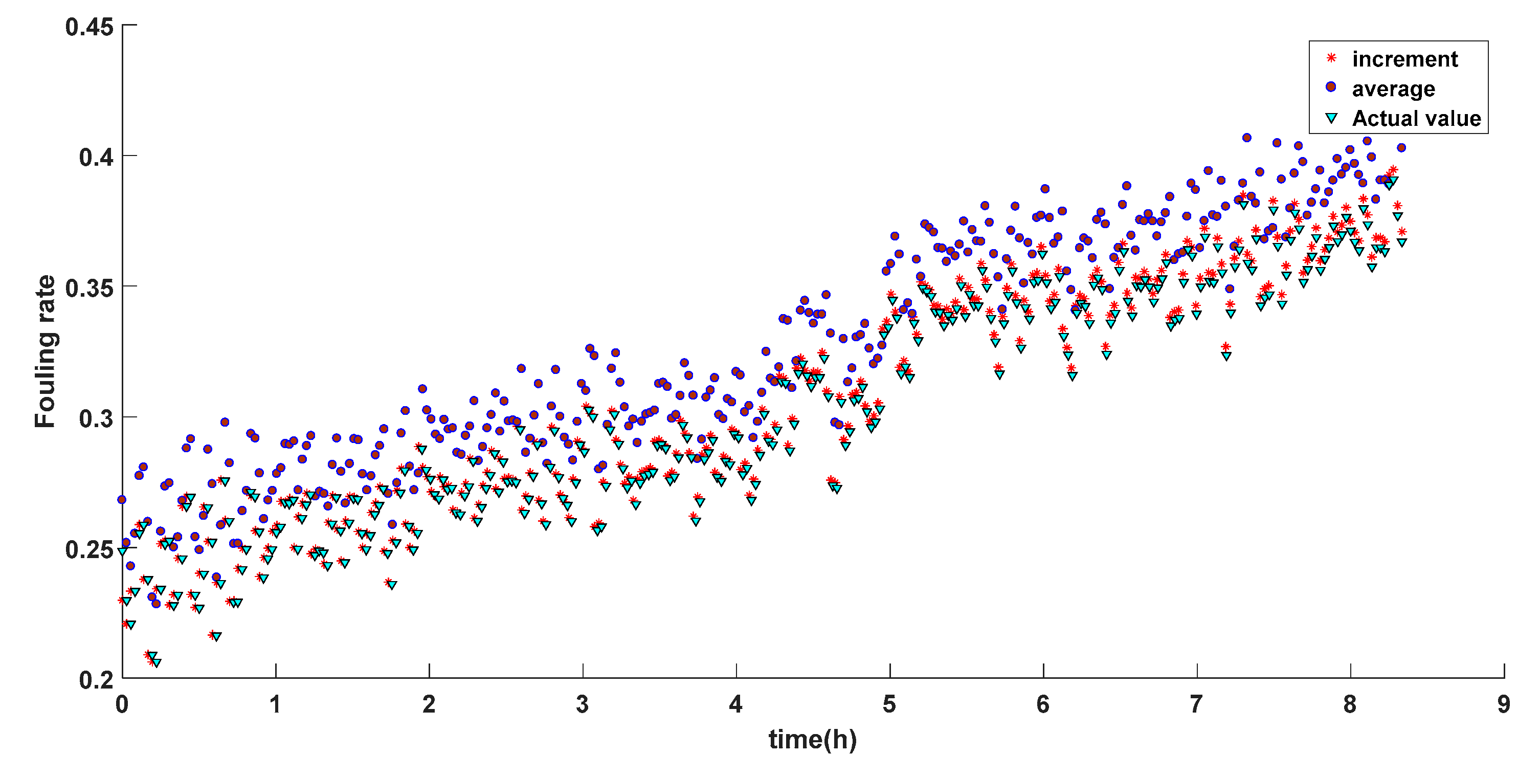
6.3. The Proposed Incremental Method

Two methods are proposed in this manuscript, mainly to get $F_d(t)$ and $F_b(t)$, respectively:

Method 1: Method based on data statistics.

In this manuscript, 20 sets of fouling rate data are used. In each set of fouling rate data, there are 300 points in the process of soot accumulation, 24 points in the process of soot blowing, and the time interval is 100 s.

Step 1: At 0 × 100 s, 20 sets of data will have 20 different fouling rates. By fitting 20 fouling rates, the probability distribution function at 0 × 100 s can be obtained. The probability density function can be obtained by derivation, and the mathematical expectation, $E(X_1)$, at 0 × 100 s can be calculated by the formula: $E(X)={\displaystyle \int f(x)xdx}$.

Step 2: At the time of 1 × 100 s, $E(X_2)$ is obtained by the same method;

……

Step n: At time n × 100 s, $E(X_n)$ is obtained.

When n = 300, the 300 mathematical expectations ($E(X_1)$, $E(X_2)$ … $E(X_{299})$) are taken as the points of the soot accumulation process, and these discrete points can be fitted by the curve to obtain $F_d(t)$.

When n = 24, the 24 mathematics expectations ($E(X_1)$, $E(X_2)$ … $E(X_{24})$) are taken as the points of the soot blowing process, and these discrete points can be fitted by the curve to obtain $F_b(t)$.

Method 1 is only applicable to partial data in which the pollution rate sequence is in the middle position, and is not applicable to all data, and there are certain deficiencies.

Method 2: Method based on incremental distribution.

The 20 sets of fouling rate data used in this manuscript have 299 time intervals (23 time intervals) for each set of fouling rate data of the soot accumulation process (soot blowing process).

Step 1: In the first time interval, in a group of data, the fouling rate at 1 × 100 s is different from that at 0 × 100 s, and the “increment of fouling rate” is obtained. By the same method, the “increment of fouling rate“ of the other 19 sets of data in the first time interval can be obtained, and then the 20 “increment of fouling rate” obtained is fitted to obtain the probability distribution (as shown in Figure 7, which obeys the normal distribution), which is called the incremental distribution.

Step 2: In the second time interval, the incremental distribution of the second time interval is obtained by the same method.

Step n: At the nth time interval, the incremental distribution of the nth time interval is obtained.

When n = 299, 299 incremental distributions of the soot accumulation stage are obtained.

When n = 23, 23 incremental distributions of the soot blowing stage are obtained.

Figure 7 is a random selection of six incremental distributions obtained. The abscissa is the fouling rate increment and the ordinate is the probability. The parameter, $\mu$, in the normal distribution is a positional parameter of the normal distribution, which is used to describe the concentrated trend position of the normal distribution. The parameter, $\sigma$, describes the degree of dispersion of the data distribution. A conclusion can be drawn from the analysis of all the incremental distributions that all parameters’ $\sigma$ are extremely small, indicating that the normal distribution is concentrated. It is reasonable to use a parameter, $\mu$, to represent the incremental data distribution. Only one initial value is given, and the initial value is superposed with 299(23) increments in turn. All the fouling rate data (300 soot accumulation points and 24 soot blowing points) in the whole soot blowing cycle are obtained. $F_d(t)$ and $F_b(t)$ can be obtained by fitting these discrete points in the process of soot accumulation and soot blowing.

Figure 8 shows the fouling rate rankings of the two groups monitored when the initial cleaning status of the economizer heating surface is different, but the operating load and the coal working condition are the same. These two sets of data are obtained from 20 sets of existing data, which are the two groups with a larger or smaller fouling rate at the beginning of economizer. The fouling rate of the heating surface will change over time, and there will always be differences in the fouling rate data between the two groups.

The data with a small initial value (the red point in Figure 8) is selected as a reference object, and the fouling rate data processed by the first method and the second method are compared with the reference object. In Figure 9, “actual value” represents the fouling rate data of the reference object; “average” represents the fouling rate data obtained by method 1; “increment” represents the fouling rate data obtained by method 2. The results obtained by the above two methods are shown in Figure 9. It can be seen from the figure that the result obtained by the first method differs greatly from the actual value. The second method is more similar to the actual value. It is obvious that the second method can reflect the actual state of the heated surface.

6.4. Calculation Examples and Analysis of Results

This manuscript calculates the optimization example of soot blowing in a boiler economizer. Because the calculation result of the economizer fouling rate is a discrete value, it cannot be directly applied to the soot blowing optimization model, and curve fitting is needed. According to the literature [23,24], the fitting form of $F_d$ and $F_b$ is as follows:

$$F_d=A-B{e}^{-Ct}$$

(25)

$$F_b=D{e}^{-Et}$$

(26)

where A, B, C, D, and E are all constants obtained by fitting and are all greater than 0. Since the thermal parameters of the boiler are extremely disturbed during operation, $t_d$ and $t_b$, calculated under different operating conditions, will be different, but the operating parameters under the same load and coal conditions are relatively stable. Therefore, the operation process of the power plant can be divided into different operating loads and coal working conditions, and the corresponding $t_d$ and $t_b$ under each operating condition can be calculated to guide the blowing operation. Taking the 300 MW of the normal operating load as an example, in order to improve the goodness of fit and reliability of the data fitting results, multiple groups of the same operating load and fouling rate data of the coal working conditions were used to fit. The specific operation flow is as follows:

Step 1: Obtain the real-time operation data of the economizer through the distributed control system (DCS).

Step 2: Through the data preprocessing, the collected operating data is used to calculate the fouling rate.

Step 3: Multiple sets of data are added at the same time to calculate the increments of multiple fouling rates at the same time, and the increase in fouling rate at the same time is calculated, and the expected increase in the fouling rate at each time is calculated.

Step 4: Take a set of initial values of the fouling rate as a starting point in the multiple sets of data and calculate the fouling rate at the subsequent time based on the expected increase in the fouling rate obtained in the third step.

Step 5: Fit the obtained fouling rate according to the time axis and calculate the goodness of fit.

Step 6: The fitting curve of the dust accumulation time period and blowing time period is brought into Equation (20), and the optimal $t_d$ and $t_b$ are obtained through the optimization algorithm. The optimization result is brought into Equation (21) and $F_{\max }$ is obtained.

Step 7: Through the optimization results obtained, the soot blowing scheme is formulated to reduce the operational burden of the operators.

Figure 10 and Figure 11 are the fouling rate rankings obtained by the incremental method during the dust accumulation and soot blowing periods, respectively. The fitting results of the two are good at 90.33% and 95.08%, respectively, and the goodness of fit is above 90%, which can be more accurately applied to soot blowing optimization calculation. The fit is as follows:

$$F_d=10.54-10.31e^{-0.001716t}$$

(27)

$$F_b=0.328e^{-0.4515t}$$

(28)

In order to satisfy the constraint requirement $F_d(t_d)=F_b(t_d)$, in the calculation, the fitting formula $F_b$ is changed to:

$$F_b=0.328e^{-0.4515(t-t_d+t_c)}$$

(29)

where $t_c$ is the intermediate parameter set to define the starting point of the fitted curve and can be eliminated by Equation (20). The fitting results of $F_d$ and $F_b$ are substituted into the soot-blowing optimization calculation model, and the $t_d$ and $t_b$ are solved by the Particle Swarm Optimization(PSO) algorithm. The definition of the soot blowing period, $t_c$, is: $t_c=t_d+t_b$.

As shown in

Table 2. Optimization calculation results of soot blowing.

Parameter	Original Value	Optimized Results	Comparison of Results
$t_d (\mathrm{h})$	8.33	7.62	0.71	9.32%
$t_b (\mathrm{h})$	0.67	0.46	0.21	46.65%
$t_c (\mathrm{h})$	9	8.08	0.92	11.39%
$F_{\min }$	0.26	0.26
$F_{\max }$	Experience setting	0.36
$Q_p (\mathrm{kJ}/\mathrm{h})$	10,750,163.25	15,570,885.17	4,820,721.92	30.96%

, the soot blowing frequency is increased in the optimization calculation result; the soot blowing period, $t_c$, is reduced from 8.33 to 7.62 h; the single soot blowing time is reduced from 0.67 to 0.46 h; and the heat exchange capacity per unit time of the economizer is increased by 4,820,721.92 $\mathrm{kJ}/\mathrm{h}$. Standard coal is a conversion standard artificially developed for the purpose of the unified calculation of the caliber. Standard coal is used as a standard for calculation or comparison. In general, judging the quality of different soot optimization strategies is achieved by comparing the standard coal consumption of different strategies. The calorific value of 1 kg standard coal is about 29,509.8 $\mathrm{kJ}$. It is equivalent to a calorific value saving of 163.36 $\mathrm{kg}/\mathrm{h}$ standard coal. Assuming that the normal working time of a coal-fired power plant is 5000 hours a year, 816.8 tons of standard coal can be saved in the economizer part of a coal-fired power plant boiler annually after the optimization of the soot blowing cycle by using the optimization method in this manuscript. The optimization effect is obvious.

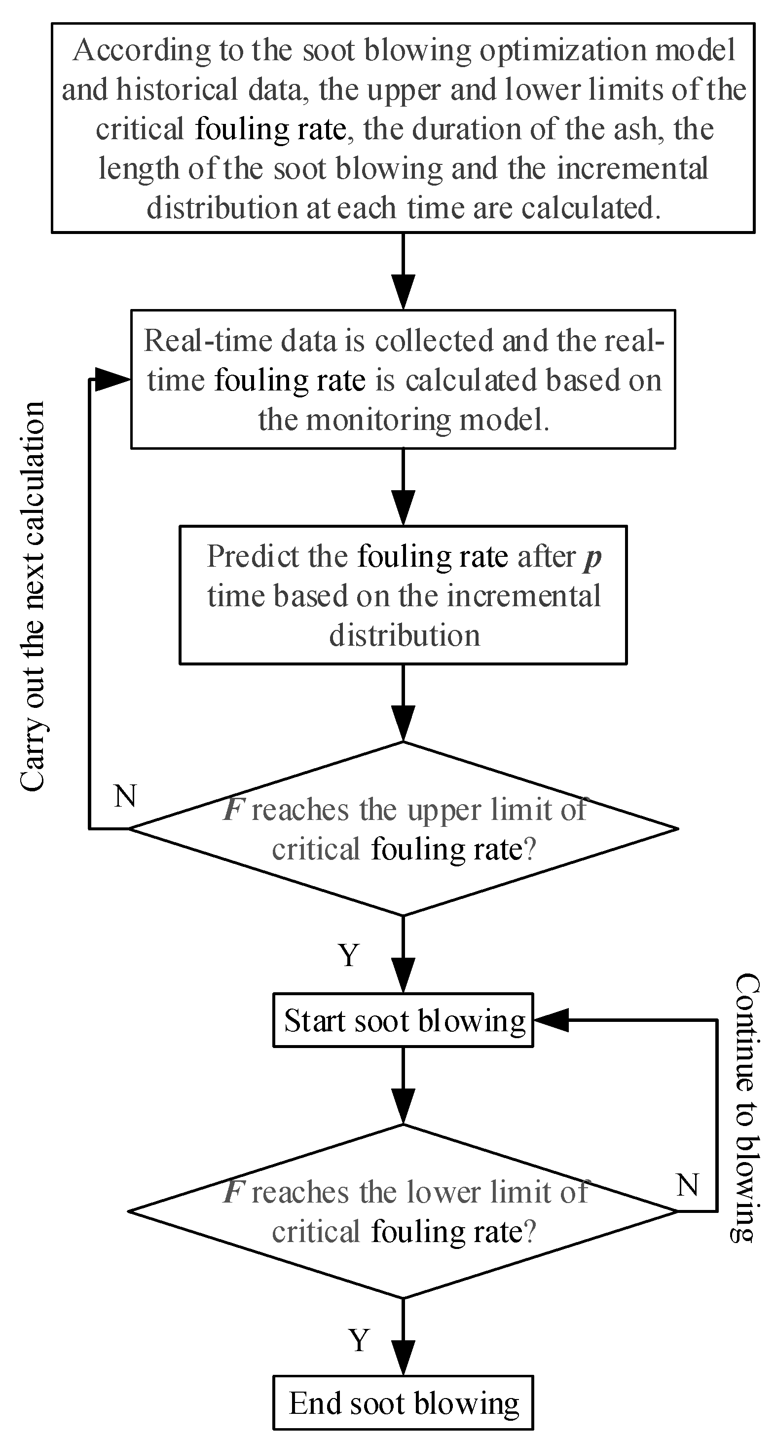
6.5. The Optimization Strategy of Soot Blowing

In this manuscript, the critical fouling rate, duration of ash accumulation, and duration of soot blowing are combined to formulate the optimal strategy for soot blowing. It is assumed that the preparation time of ash blowing operation is p, as shown in Figure 12.

The actual soot blowing operation of an economizer in a power plant also needs to take into account the main steam and reheat steam temperature, superheater and reheater desuperheating water flow, load standards and smoke exhaust standards, and other power plant indicators. The actual optimization strategy of soot blowing of the power plant can be modified based on the optimization scheme developed in this manuscript.

7. Conclusions

In this manuscript, the boiler efficiency and steam loss caused by soot blowing were weighed, and an optimization model of soot blowing per unit time heat transfer was proposed to improve the economic benefit of coal-fired utility boilers. The optimization variables of the optimization model are the soot blowing period (soot accumulation time, $t_d$, and soot blowing time, $t_b$), and the soot accumulation curve, $F_d$, and soot blowing curve, $F_b$, in the optimization model are also unknown. In order to obtain the ash accumulation curve, $F_d$, and the soot blowing curve, $F_b$, a method based on incremental distribution was proposed in this manuscript. In this method, the incremental distribution curves of all time intervals are obtained by using multiple sets of fouling rate data at the same working condition and the same measuring point. By analyzing the incremental distribution of all time intervals, the increments of all time intervals are obtained. Under the condition of a known initial heating surface clean state (fouling rate), the fouling rate at all times in the soot blowing cycle can be obtained by using the cumulative method. These fouling rates are discrete points and cannot be used directly. For this reason, the curve fitting method was used for these discrete points to obtain the ash accumulation curve, $F_d$, and the soot blowing curve, $F_b$, which are in the soot blowing optimization model. The PSO optimization algorithm was used to maximize the heat transfer of the heated surface in a unit of time, and the optimum soot blowing period (soot accumulation time, $t_d$, and soot blowing time, $t_b$) was obtained. A simple soot blowing optimization strategy was formulated based on the optimum soot blowing period. The results show that 816.8 tons of standard coal can be saved per year if the heating surface of the economizer of a 300 MW coal-fired power plant boiler is taken as the research object and the normal working time of the coal-fired power plant is 5000 hours per year. The optimization strategy can be used to guide soot blowing operation and improve boiler performance. It can not only improve heat transfer efficiency but also reduce unnecessary steam waste.

References

1. Sivathanu, A.K.; Subramanian, S. Extended Kalman filter for fouling detection in thermal power plant reheater. Control. Eng. Pract 2018, 73, 91–99. [Google Scholar] [CrossRef]
2. Sandberg, J.; Fdhila, R.B.; Dahlquist, E.; Avelin, A. Dynamic simulation of fouling in a circulating fluidized biomass-fired boiler. Appl. Energy 2011, 88, 1813–1824. [Google Scholar] [CrossRef]
3. Dong, M.; Han, J.; Li, S.; Pu, H. A Dynamic Model for the Normal Impact of Fly Ash Particle with a Planar Surface. Energies 2013, 6, 4288–4307. [Google Scholar] [CrossRef]
4. Shao, Y.; Wang, J.; Preto, F.; Zhu, J.; Xu, C. Ash Deposition in Biomass Combustion or Co-Firing for Power/Heat Generation. Energies 2012, 5, 5171–5189. [Google Scholar] [CrossRef]
5. Romeo, L.M.; Gareta, R. Neural network for evaluating boiler behaviour. Appl. Therm. Eng. 2006, 26, 1530–1536. [Google Scholar] [CrossRef]
6. Aliakbari, S.; Ayati, M.; Osman, J.H.; Sam, Y.M. Second-order sliding mode fault-tolerant control of heat recovery steam generator boiler in combined cycle power plants. Appl. Therm. Eng. 2013, 50, 1326–1338. [Google Scholar] [CrossRef]
7. Romeo, L.M.; Gareta, R. Fouling control in biomass boilers. Biomass Bioenergy 2009, 33, 854–861. [Google Scholar] [CrossRef]
8. Pena, B.; Teruel, E.; Diez, L. Soft-computing models for soot-blowing optimization in coal-fired utility boilers. Appl. Soft Comput. 2011, 11, 1657–1668. [Google Scholar] [CrossRef]
9. Dong, M.; Li, S.; Xie, J.; Han, J. Experimental Studies on the Normal Impact of Fly Ash Particles with Planar Surfaces. Energies 2013, 6, 3245–3262. [Google Scholar] [CrossRef]
10. Teruel, E.; Cortés, C.; Díez, L.I.; Arauzo, I. Monitoring and prediction of fouling in coal-fired utility boilers using neural networks. Chem. Eng. Sci. 2005, 60, 5035–5048. [Google Scholar] [CrossRef]
11. Perez, L.; Ladevie, B.; Tochon, P.; Batsale, J. A new transient thermal fouling probe for cross flow tubular heat exchangers. Int. J. Heat Mass Transf. 2009, 52, 407–414. [Google Scholar] [CrossRef] [Green Version]
12. Qiu, K.; Zhang, H.; Zhou, H.; Zhou, B.; Li, L.; Cen, K. Experimental investigation of ash deposits characteristics of co-combustion of coal and rice hull using a digital image technique. Appl. Therm. Eng. 2014, 70, 77–89. [Google Scholar] [CrossRef]
13. Kalisz, S.; Pronobis, M. Investigations on fouling rate in convective bundles of coal-fired boilers in relation to optimization of sootblower operation. Fuel 2005, 84, 927–937. [Google Scholar] [CrossRef]
14. Barrett, R.E.; Tuckfield, R.C.; Thomas, R.E. Slagging and Fouling in Pulverized-Coal-Fired Utility Boilers; A Survey and Analysis of Utility Data: Final Report; EPRI: Palo Alto, CA, USA, 1987; Volume 1. [Google Scholar]
15. Pattanayak, L.; Ayyagari, S.P.K.; Sahu, J.N. Optimization of sootblowing frequency to improve boiler performance and reduce combustion pollution. Clean Technol. Environ. Policy 2015, 17, 1897–1906. [Google Scholar] [CrossRef]
16. Valero, A.; Cortés, C. Ash fouling in coal-fired utility boilers. Monitoring and optimization of on-load cleaning. Prog. Energy Combust. Sci. 1996, 22, 189–200. [Google Scholar] [CrossRef]
17. Fan, Q.; Yan, W. Boiler Principles; China Electric Power Press: Beijing, China, 2007. [Google Scholar]
18. Shi, Y.; Wang, J.; Liu, Z. On-line monitoring of ash fouling and soot-blowing optimization for convective heat exchanger in coal-fired power plant boiler. Appl. Therm. Eng. 2015, 78, 39–50. [Google Scholar] [CrossRef]
19. Zhang, S.; Shen, G.; An, L.; Li, G. Ash fouling monitoring based on acoustic pyrometry in boiler furnaces. Appl. Therm. Eng. 2015, 84, 74–81. [Google Scholar] [CrossRef]
20. GB/T 10184-88. Performance Test Code for Utility Boiler; Chinese GB Standard: Beijing, China, 1988. [Google Scholar]
21. Shi, Y.; Wang, J.; Wang, B.; Zhang, Y. Real-time online monitoring of thermal efficiency in coal-fired power plant boiler based on coal heating value identification. Int. J. Model. Identif. Control 2013, 20, 295. [Google Scholar] [CrossRef]
22. Yan, W.; Chen, B.; Liang, X.; Xue, Y.E.; Wang, L.; Zhao, B. Investigation on Ash Monitoring Model for Rotary Air Heater in Utility Boiler. Power Eng. 2002, 22, 1708–1710. [Google Scholar]
23. Pena, B.; Teruel, E.; Diez, L. Towards soot-blowing optimization in superheaters. Appl. Therm. Eng. 2013, 61, 737–746. [Google Scholar] [CrossRef]
24. Shi, Y.; Wen, J.; Cui, F.; Wang, J. An Optimization Study on Soot-Blowing of Air Preheaters in Coal-Fired Power Plant Boilers. Energies 2019, 12, 958. [Google Scholar] [CrossRef]
Figure 1. The curve of the fouling rate in one cycle.
Energies 12 02901 g001
Figure 2. Change of the quantity of heat exchange on the heated surface.
Energies 12 02901 g002
Figure 3. Change curve of the fouling rate in multiple periods.
Energies 12 02901 g003
Figure 4. Contrast picture of the fouling rate data before (up) and after (down) pretreatment.
Energies 12 02901 g004
Figure 5. The curve of fouling rate (24 h).
Energies 12 02901 g005
Figure 6. Data of fouling rate. (a) Fouling rate data of the ash deposition process; (b) Fouling rate data for soot blowing process.
Energies 12 02901 g006aEnergies 12 02901 g006b
Figure 7. The histogram of the incremental distribution.
Energies 12 02901 g007
Figure 8. Two sets of fouling rates.
Energies 12 02901 g008
Figure 9. Results obtained by the two methods.
Energies 12 02901 g009
Figure 10. Fouling rate and fitting curve of the dust accumulation time period with time.
Energies 12 02901 g010
Figure 11. Fouling rate and fitting curve of the soot blowing time period as a function of time.
Energies 12 02901 g011
Figure 12. The optimization strategy of soot blowing.
Energies 12 02901 g012