Article

Remaining Useful Life Prediction of Rolling Element Bearings Using Supervised Machine Learning

1
Faculty of Computing, Engineering and media, De Montfort University, Leicester, LE1 9BH, UK
2
Faculty of Engineering, Environment and Computing, Coventry University, Coventry CV1 2JH, UK
3
Department of Engineering and Applied Science, School of Water, Energy and Environment, Cranfield University, Bedfordshire, MK43 0AL, UK
4
Department of Mechanical Engineering, University of Lagos, Nigeria 100213, West Africa
*
Author to whom correspondence should be addressed.
Energies 2019, 12(14), 2705; https://doi.org/10.3390/en12142705
Submission received: 9 June 2019 / Revised: 5 July 2019 / Accepted: 11 July 2019 / Published: 15 July 2019
(This article belongs to the Special Issue Fault Diagnosis and Fault-Tolerant Control)

Abstract

:
Components of rotating machines, such as shafts, bearings and gears are subject to performance degradation, which if left unattended could lead to failure or breakdown of the entire system. Analyzing condition monitoring data, implementing diagnostic techniques and using machinery prognostic algorithms will bring about accurate estimation of the remaining life and possible failures that may occur. This paper proposes a combination of two supervised machine learning techniques; namely, the regression model and multilayer artificial neural network model, to predict the remaining useful life of rolling element bearings. Root mean square and Kurtosis were analyzed to define the bearing failure stages. The proposed methodology was validated through two case studies involving vibration measurements of an operational wind turbine gearbox and a split cylindrical roller bearing in a test rig.

1. Introduction

Rolling element bearings are critical components in rotating machinery. These bearings generally operate under adverse conditions, making performance degradation unavoidable. Such degradation, if left unattended, can cause failure or breakdown of the entire system. The purpose of prognostics is to use prediction techniques to predict the remaining useful life (RUL) of a system and its constituent components based upon historical information, current usage and future operating conditions so as to prevent the catastrophe from happening [1]. Historical information includes historical failure data of similar systems and event logs. Current usage could be in the form of a feature derived from sensor measurements which indicates the current health status of the system. Future operating condition refers to operational and environmental factors that could affect the future status of the system. Such information can be obtained based on expert opinion or by looking at the production plans. Prognostics offers several benefits, including [2,3]:
  • Avoiding catastrophic failure, unscheduled maintenance and production loss.
  • Reducing maintenance costs by minimizing the number of unnecessary interventions and machine overhauls.
  • Increasing the lifespan of components by providing advance information on the severity of the fault to be maintained.
The RUL of a bearing is generally defined either as the total number of revolutions before a failure occurs or the total number of hours that the bearing can run until the first sign of failure develops [4]. The RUL is estimated based on measured and calculated bearing condition variables such as vibration amplitude and frequency. As shown in Figure 1, if a certain condition indicator x is calculated or monitored continuously from t = 0 to t = t B , then a continuous time series y(t) can be obtained, which represents the deterioration process of the component under study. This time series consists of two parts, α and β, which indicates the healthy running stage and the fault degradation stage, respectively. Prognostic analysis is usually based on the analysis of the time series from point A to point B. Ideally, if the RUL of a bearing (i.e., the total running time between point A to B) can be accurately estimated by using only the past data covered by α, then the optimal maintenance schedule can be made easily.
Over recent decades, much research has been implemented to develop health monitoring methods for rotating machinery, especially bearings. Compared to fault detection, the literature of prognostics and health management is relatively limited, and effective implementing of prognostic techniques is still lacking. The increased interest in machinery prognostics has resulted in many successful tools, models and applications in the past few years. Basically, there are three types of prognostic approaches that can be employed to predict the RUL; namely, data-driven methods, physics-based models and hybrid models. Data-driven approaches utilize the historical failure data of the machine and/or similar machines to estimate how much time is left until a system malfunction occurs. This method does not require an in-depth understanding of the physics of systems under study. Physics-based approaches predict the remaining life according to propagation of the damage mechanism (i.e., physics of failure). A hybrid approach uses both a data-driven and physics-based method so as to achieve an improved predictive performance in terms of a more improved predictive accuracy than that of the single method.
Over recent years, many efforts have been conducted in developing regression-based prognostic methods that can be used to estimate the RUL of rotating machinery. Li et al. [5] improved the performance of the traditional exponential regression model and applied the developed regression model to vibration measurements collected from rolling element bearings to predict RUL. Wu et al. [6] put forward a time-to-failure prognostic method based on an empirical Bayesian algorithm and exponential regression model for rolling element bearings. Sutrisno et al. [7] investigated the accuracy of three different techniques for predicting the RUL of bearings. Bayesian Monte Carlo and moving average spectral kurtosis, support vector regression (SVR) and an anomaly detection algorithm were compared according to their performance in estimating a ball bearing’s remaining life. The anomaly detection technique was found to be the most accurate among all methods compared. Goebel et al. [8] conducted a comparative study of three prognostic methods: relevance vector machine (RVM), Gaussian process regression (GPR) and a neural network. The study showed that the three techniques have resulted in significant different RUL prediction results. Loukopoulos et al. [9] studied the performance of several machine learning techniques, including linear regression, polynomial regression and K-Nearest Neighbors Regression. The results showed that an ensemble method based on the weighted average of the predicted RUL of each individual method offers a higher predictive accuracy. Kim et al. [10] utilized Support Vector Regression to evaluate the bearing health condition by using real-world run-to-failure data obtained from bearings of gas pumps. The results showed that the developed probability estimation based prognostic method is potentially very effective for RUL prediction.
Several other artificially intelligent approaches applied to machinery prognostics have been considered by researchers. For instance, a self-organizing neural network was employed by Zhang and Ganesan [11] for extrapolating the fault progression and estimating the remnant life of a bearing. Loukopoulos et al. [9] applied a Self-Organizing Map (SOM) model to predict the RUL of industrial pumps using temperature measurements. Dong et al. [12] developed a condition prediction method based on the grey model and back-propagation neural network. Elasha et al. [13] put forward a life assessment approach for tidal turbine gearboxes. The method was validated on data generated using a Blade Element Momentum Theory (BEMT) model. They predicted the RUL of a gearbox based on the turbine loading conditions. The results of their investigation show life variations between the gears due to differences in stress cycles and differing rotational speeds. Li et al. [14] put forward a hybrid method in which a long short-term memory model and a state-space model was combined to predict the pro-fault performance of a centrifugal compressor. An adaptive neuro-fuzzy inference system (ANFIS) was used together with the particle filtering (PF) algorithm in [15] to predict the RUL of a gearbox. The authors concluded that the ANFIS model outperforms the recurrent neural network through a comparative study. Elforjani and Shanbr [16] employed three supervised machine learning techniques; Artificial neural network (ANN), SVR and GPR, to correlate Vibration measurement features with natural wear of bearings. They concluded that the back-propagation neural network model outperforms the other methods in predicting the RUL of bearings. The aforementioned prognostic techniques offer a tradeoff between reliability, speed and applicability. This paper combines two supervised machine learning techniques; namely, the regression model and artificial neural network (ANN) model to correlate vibration features with the corresponding fault stages during the natural run-to-failure process of rolling element bearings. The main contribution of this study is to improve the fitting of condition indicators obtained from vibration signals of bearings using appropriate regression models. Furthermore, this study aims to ascertain the feasibility of using ANN models to estimate the RUL of rolling element bearings, and to explore the feasibility of combining regression models with ANNs for a better RUL prediction. The effectiveness of the hybrid prognostic method was validated through two case studies: an operational wind turbine gearbox and a split cylindrical roller bearing used in an experimental test rig.

2. Methodology

Contributions

In condition monitoring applications, the vibration signals of bearing damage often present multiple modulation characteristics, and therefore the features extracted by the general methods from one bearing may not necessarily correlate to fault characteristics extracted from another bearing. The internal reasons behind this include, for example, different observed trends from different cases. As a result, there is still a need to apply and validate bearing fault indicators such as root mean square (RMS) and Kurtosis (KU) for different applications. Furthermore, due to the measurement noise, variation of operating conditions and stochasticity of the system deterioration, the extracted condition indicators from the raw vibration signals generally contain fluctuations, which would incur inaccurate RUL predictions. In this context, this study contributes to the existing literature in that:
  • It improves the fitting of the features extracted from vibration measurements through the use of appropriate regression models.
  • It explores the possibility of combining regression models with ANNs to improve the predictive accuracy of regression models.
  • A test rig was designed and experimental tests were conducted to generate bearing failure data in order to validate the proposed prognostic model. The model was also validated through industrial data provided by a commercial company.

3. Statistical Condition Indicators

Vibration based health monitoring schemes are applicable for monitoring many constituent components of a gearbox, such as shafts, gears and bearings. To achieve a better signal-to-noise ratio (SNR), vibration measurements are processed using filtering and amplifying techniques. Two condition indicators, RMS and KU [17], are often generated from the vibration signals. Then the extracted condition indicators are fitted using regression methods to provide useful information about the bearing degradation.

3.1. Kurtosis

Each mechanical failure has an associated “signature” that can be found in the frequency or time domain representations of vibration signals. Kurtosis is such a “signature” which is referred to as the fourth statistical moment of a given signal, reflecting the peakness of the histogram [18]. A kurtosis value greater than three is an indicator of a sharp peak signal. A kurtosis value smaller than three indicates vibration signals with flat peaks. In some cases, the occurrence of background noise and other sources of vibration signals may prevent bearing faults from being detected through the observation of changes in the kurtosis. To solve this problem, the kurtosis value needs to be computed across different frequency bands [19]. The Kurtosis of a random signal is computed as:
K U   =   1 N i   =   1 N ( X i   μ ) 4 [ 1 N i   =   1 N ( X i   μ ) 2 ] 2
where N is the number of samples in the signal, X i refers to the amplitude of the signal of the i th sample, and μ denotes the mean sample amplitude.

3.2. Root Mean Square

The root mean square (RMS) value describes the energy content of a signal. RMS is one of the most commonly used statistical parameters that describe change in the dynamic of the machine [20]. For the signal of sample size N , the RMS value is calculated using the equation below.
R M S   =   X 1 2 + X 2 2 + X N 2 N
It is well known that the RMS value is a weak method to detect failure at its early stage because of the small energy generated by the defect, which makes a small difference in the value of RMS. However, RMS is capable of reflecting the increase of the vibration energy as the fault progresses [5]. Consequently, RMS is employed as the prediction indicator in this study. In other words, the RUL is predicted by extrapolating the trajectory of RMS values.

4. Regression Analysis

Regression models, as one of the most popular data-driven techniques for RUL prediction, make attempts at fitting available data of deterioration by regression functions and then extrapolating the fault propagation until the fitted curve reaches a pre-defined threshold. The objective of regression analysis is to find an empirical relation to predicting the bearing degradation thought time series. Due to measurement noise, variation of operational conditions and the stochastic nature of the degradation processes, the acquired data are usually accompanied by fluctuations that may have a significant impact on the model’s ability to interpret the degradation trend. In this case, the raw condition indicators cannot be directly used as the inputs of the prediction models. This is due to the fact that any fluctuations in the condition indicators will cause the model to follow the randomness, and consequently, its ability to accurately estimate the health status of the bearings may be very weak [21]. Therefore, in this study, we first conduct a comparative study of two regression models, namely polynomial and exponential regression, and then choose the one with the best fitting performance to fit the condition indicators extracted from the data.
The polynomial models are suitable for situations where the correlation between explanatory and study variables is curvilinear. Polynomial regression belongs to the least-square curve fitting family. It takes a set of data as inputs and generates an approximation between the input data and time. To be specific, it estimates the coefficients of a polynomial function in that the function approximates the curve closely. The formula of polynomial regression is as follows:
y 1 = a 0 + a 1 x + a 2 x 2 + + a n x i n
where y 1 is the response variable, χ is the predictor variable, and a 0 ,   a 1 ,…, a n are model coefficients. The degree of the polynomial function is determined by the number of non-zero coefficients in (3), which in turn determines how accurate the data can be fit. If the number of coefficients is zero or one, then the fitted curve is known as a linear regression. If the number of coefficients is larger than one, a non-linear polynomial regression will be implemented.
The exponential regression model involves a fitting process that finds the parameters of the exponential function which can present the best fit for a set of data [21]. The function form of the exponential is shown in Equation (4):
y 2   =   a   ×   e b x
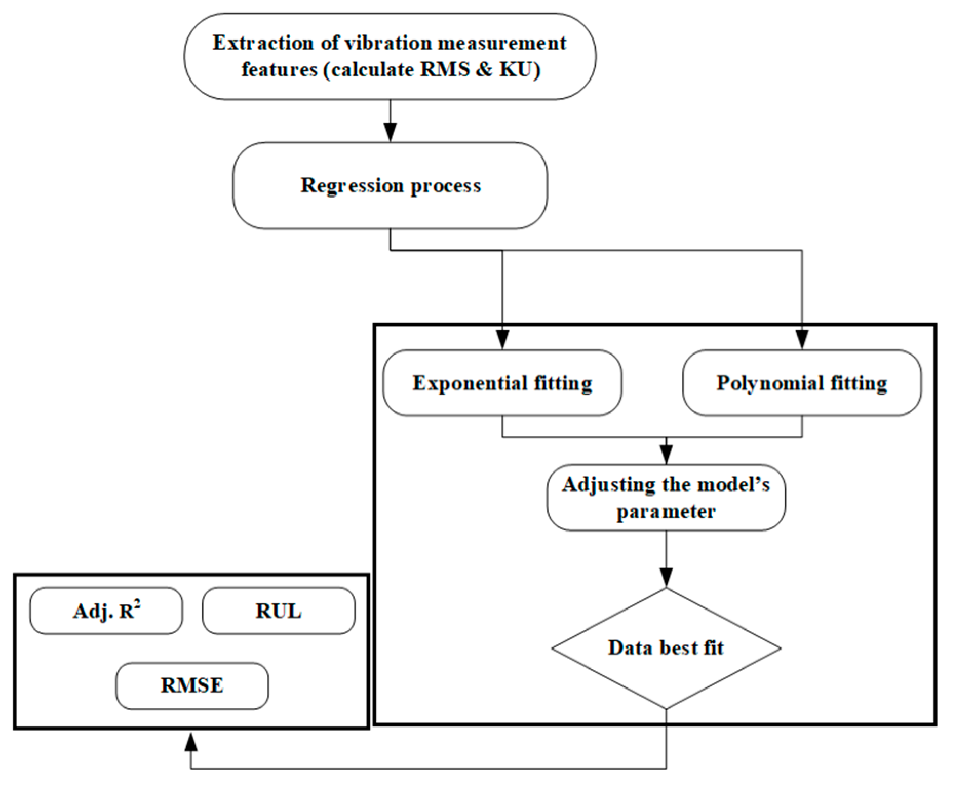
where a , b are model constants and χ is the predictor variable. Figure 2 shows the process of using the two regression models to find the best fit of the condition indicators. The vibration signals were first processed to obtain the condition indicators; namely, RMS and KU. Then the coefficients in Equations (3) and (4) are determined such that the best fit of the exponential and polynomial functions are reached. The performance of the regression models has been assessed using two statistics: root mean square error (RMSE) and adjusted R2. The RMSE is defined as the square root of the variance of the residuals between the predicted and the actual RUL. RMSE measures how close the measured data is to the predicted values. The R2 is defined as the ratio between the difference between the sum square total (SST) and sum square error (SSE) to the SST. SST measures the data deviation from the sample mean, and SSE measures the deviation of the data from the model’s predicted values. One of the disadvantages of the R2 metric is that it does not indicate if a regression model provides an adequate fit to the data. Therefore, the adjusted R2 was instead used in this research as the third performance metric. Adjusted R2 is defined as the ratio between the residual mean square errors to the total mean square error (which is the variance of the predicted values).

5. Multilayer Artificial Neural Network

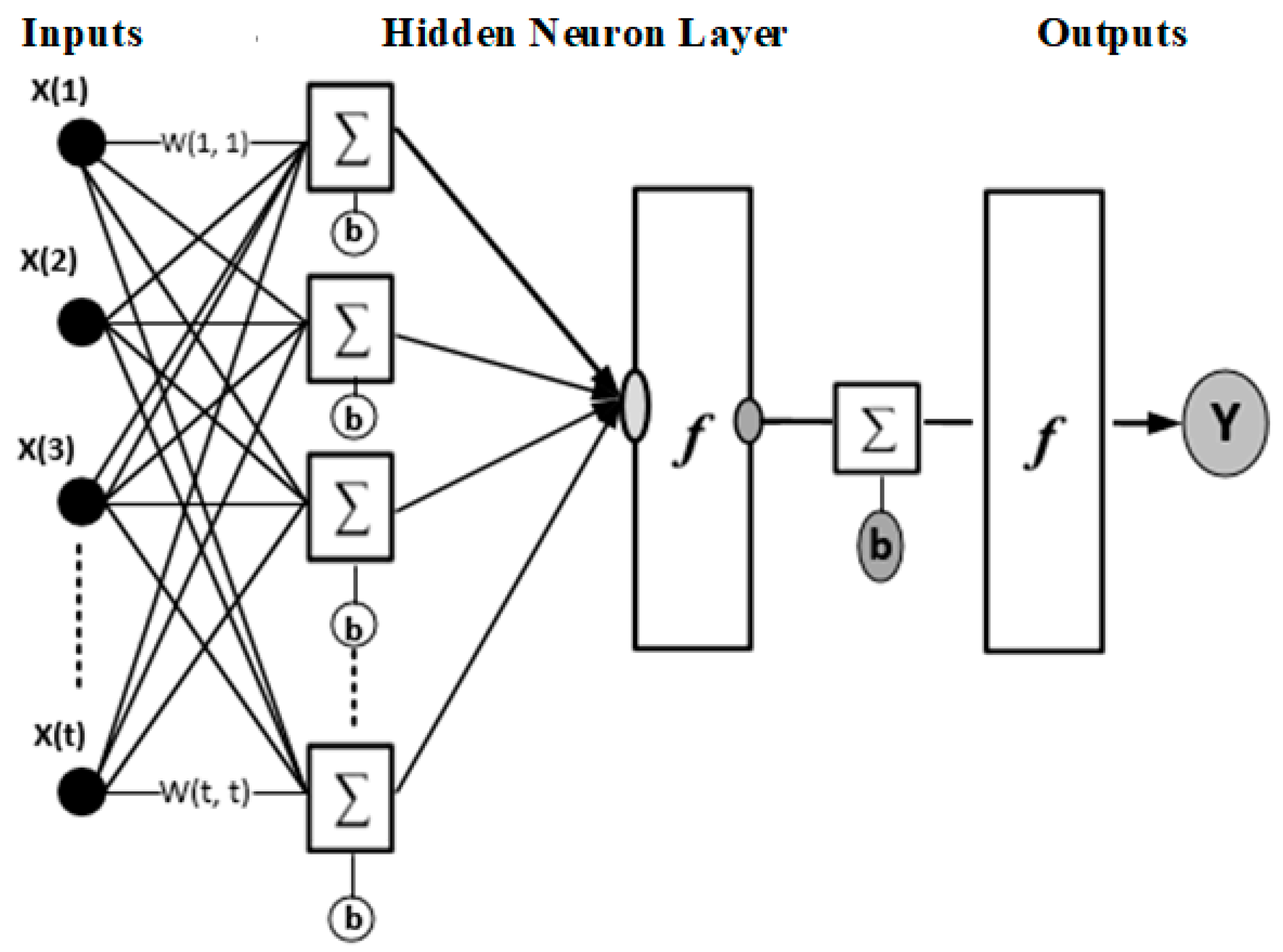
ANNs belong to the supervised machine learning family. They are inspired by biological neural networks and each neuron is represented by a node [22]. An ANN generally contains an input layer, multiple hidden layers, one output layer, biases and connection nodes. When the known inputs and target outputs are repetitively presented to an ANN, the connection weights between nodes will be adjusted automatically such that the difference between the network outputs and the targets is as small as possible. In this study, the ANN that we implemented is a multilayer back-propagation neural network. Figure 3 illustrates an exemplary architecture of the multiple-layer neural network model. It is observable from the figure that each layer consists of its own input and output nodes (x & y), weighting coefficients (w) and bias vector (b). The input layer doesn’t involve any processing and is utilized to directly feed information to the subsequent network layers.
In contrast, the output layer involves weighting and biases calculations when producing the network outputs. The hidden layers aim at adding additional processing so as to avoid solutions that do not converge. As shown in Figure 4, the main purpose of the bias neurons is to prevent the network from generating zero results even if the network inputs are not zero. The exemplary network structure is formed of a feed-forward model. The following equation explains how the network inputs are correlated with the outputs:
  h i   =   φ 0   [ C φ h ( B u i + b h ) +   b 0 ]
where h i is the network output vector and the input vector is represented by u i , C denotes the weighting matrix between the hidden layer and the output layer. B is the connection matrix from the input layer to the hidden layer. The bias vectors of the hidden and output layers are represented by bh and bo, respectively. φh and φo denote the activation functions of the nodes in the hidden and output layers, respectively. Feedforward neural network models also take the form of
  h i   =   f ( u )
where f (⋅) denotes a nonlinear transformation from u to h i . Interestingly, the structure of a feedforward neural network is similar to that of a nonlinear regression model. Levenberg Marquardt (LM) learning algorithm [23] was chosen as the network training function in this study for adjusting the weighting and bias matrices during the training process. Levenberg-Marquardt optimization has been applied intensively for feedforward neural network training and has been proven to be able to deal with many difficult and diverse problems in practice. This algorithm minimizes functions that are sums of squares of nonlinear functions. One of the advantages of this optimization method is that the second-order convergence point can be approached without calculating the Hessian matrix.

6. Data Collection

The proposed approach was validated on two datasets: vibration signals captured from a high-speed shaft bearing of a 2 MW wind turbine and a split cylindrical roller bearing in a test rig.

6.1. Dataset 1

The first vibration dataset was collected from the Green Power Monitoring Systems [24]. The data was collected from a high-speed shaft bearing mounted inside a 2 MW wind turbine. The high-speed bearing which is the subject of this study is housed on the tail end of a gearbox. The bearing defect was efficiently detected by the sensor which was mounted radially onto the bearing support ring. An inspection of the bearing later showed that the inner race was cracked. The crack length was 26 mm in the outer race. The vibration measurement was taken for 50 consecutive days using MEMS-based accelerometers mounted radially on the bearing support ring [24]. Data was collected at 10-min intervals. The bearing speed was 1800 rpm. A total number of 50 data sets were recorded for analysis. The vibration data was sampled at a sampling rate of 97,656 Hz for 6 s [24]. Table 1 lists the key parameters of interest.

6.2. Dataset 2

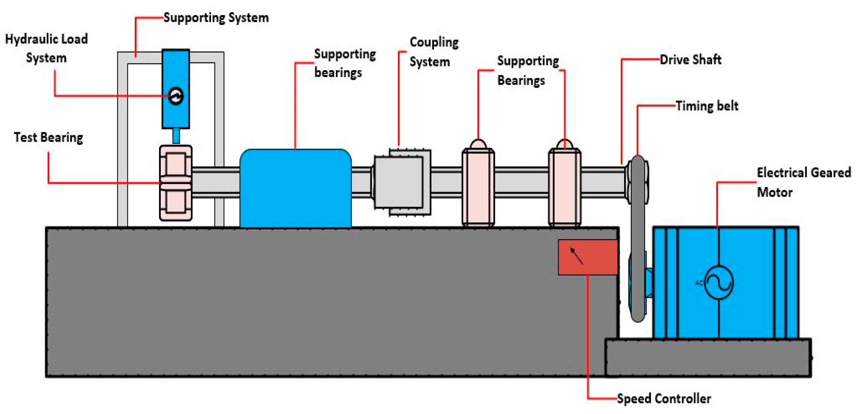
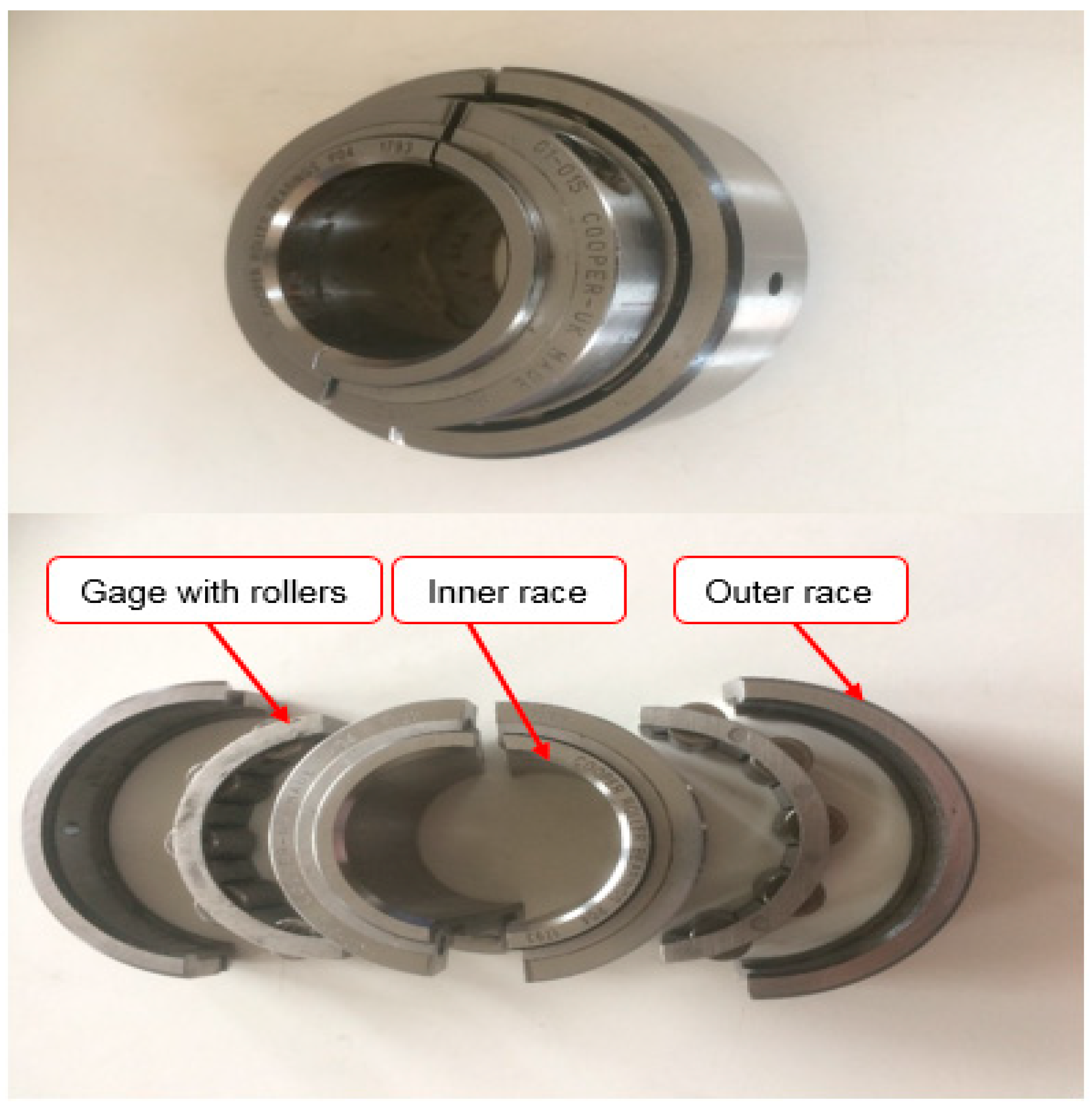
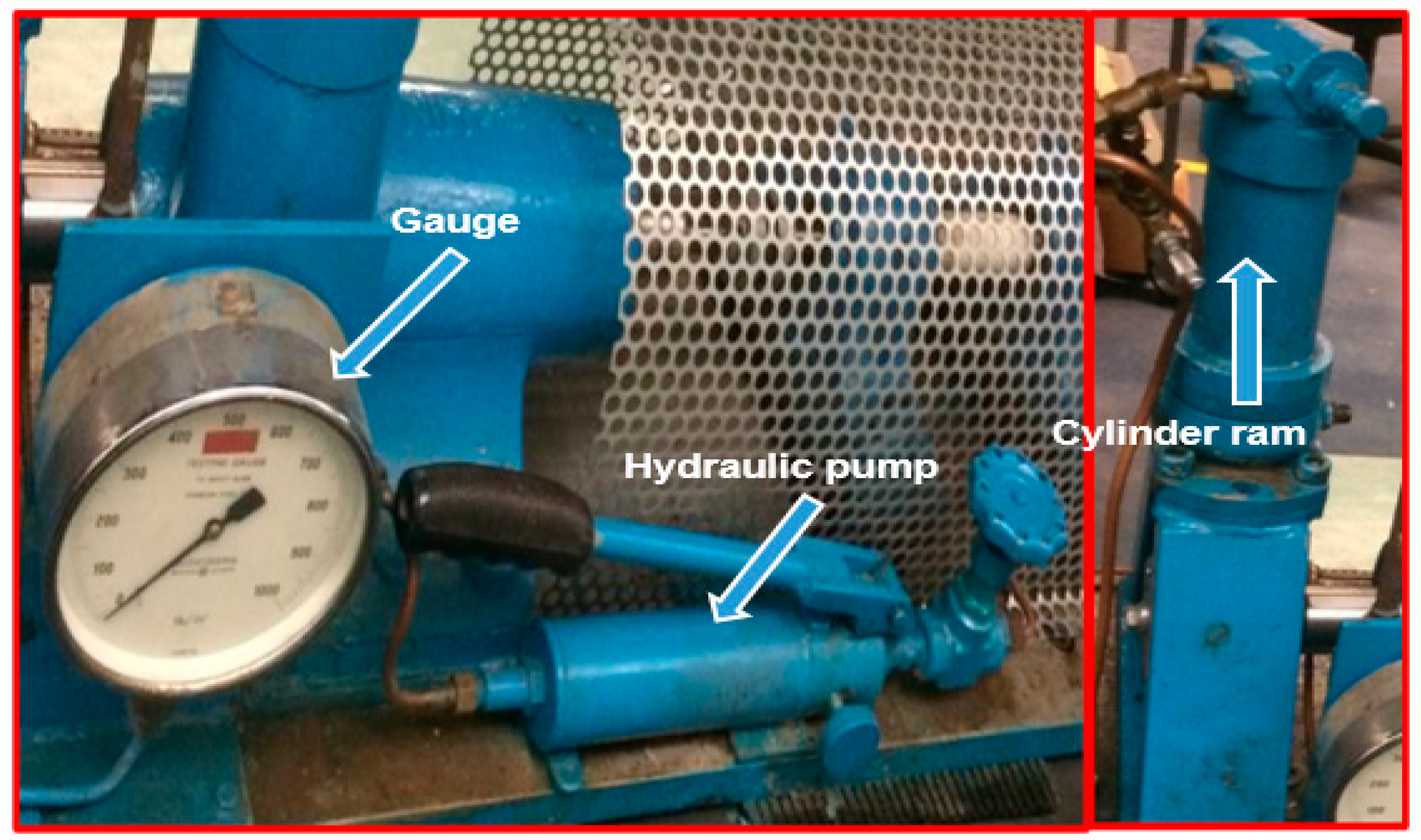
The second dataset was captured from an experimental test rig. The schematic of the test rig is shown in Figure 4. It was used to investigate the use of vibration signals to diagnose incipient bearing failure under conditions of high speed and under constant load. An electric motor (DC Motor—DY1815-B) is part of the rig. The motor drive shaft can rotate at controlled speeds between 10 and 4000 rpm. Two PZE accelerometers, each with a useful frequency range of at least 15 kHz, were attached to the test bearing housing, one mounted radial and horizontal, the other radial and vertical, to measure vibration in both directions. A split cylindrical roller bearing (type 01B 40MM GR) was employed to perform the run-to-failure test. The reason why this type of bearing was selected was that it can be mounted and dismounted simply, permitting regular inspection of the test bearing throughout the test series. As shown in Figure 5, each element of the test specimen was split into two halves. The dimensions of the test specimen are shown in Table 2. A handheld tachometer was employed to measure the shaft speed. The test load on the roller bearing was applied as normal to the driven shaft and radially to the designated load point; see Figure 6. A hydraulic ram was used to apply the test load, which was powered by a hand-pump; the magnitude of the pressure in the ram was measured using the fitted pressure gauge.
A hydraulic cylinder ram provided the radial load on the specimen housing. It was supported by an H-frame and had a gauge displaying the load value; see Figure 6. A high-accuracy data acquisition DAQ was used to record and monitor the vibration signal. The DAQ recorded all of the measurements at a sampling rate of 25.6 kHz
The accelerated life test was performed on the bearing to obtain vibration measurements during the bearing’s entire lifecycle from beginning to final failure. The Virtual Instrument (VI), consisting of a computer equipped with LabVIEW programme connected to data acquisition with sensors, was used to acquire and display vibration data. To speed up the crack initiation, a small amount of grease was applied to the roller bearing. It is worth knowing that the quantity of grease was not measured by weight nor volume. The purpose of doing this was to simulate real-world situations where the amount of lubricant inside the bearing during operation can be hard to measure and control because bearing location and geometry can make accessibility difficult.

7. Results

7.1. Signal Features Regression

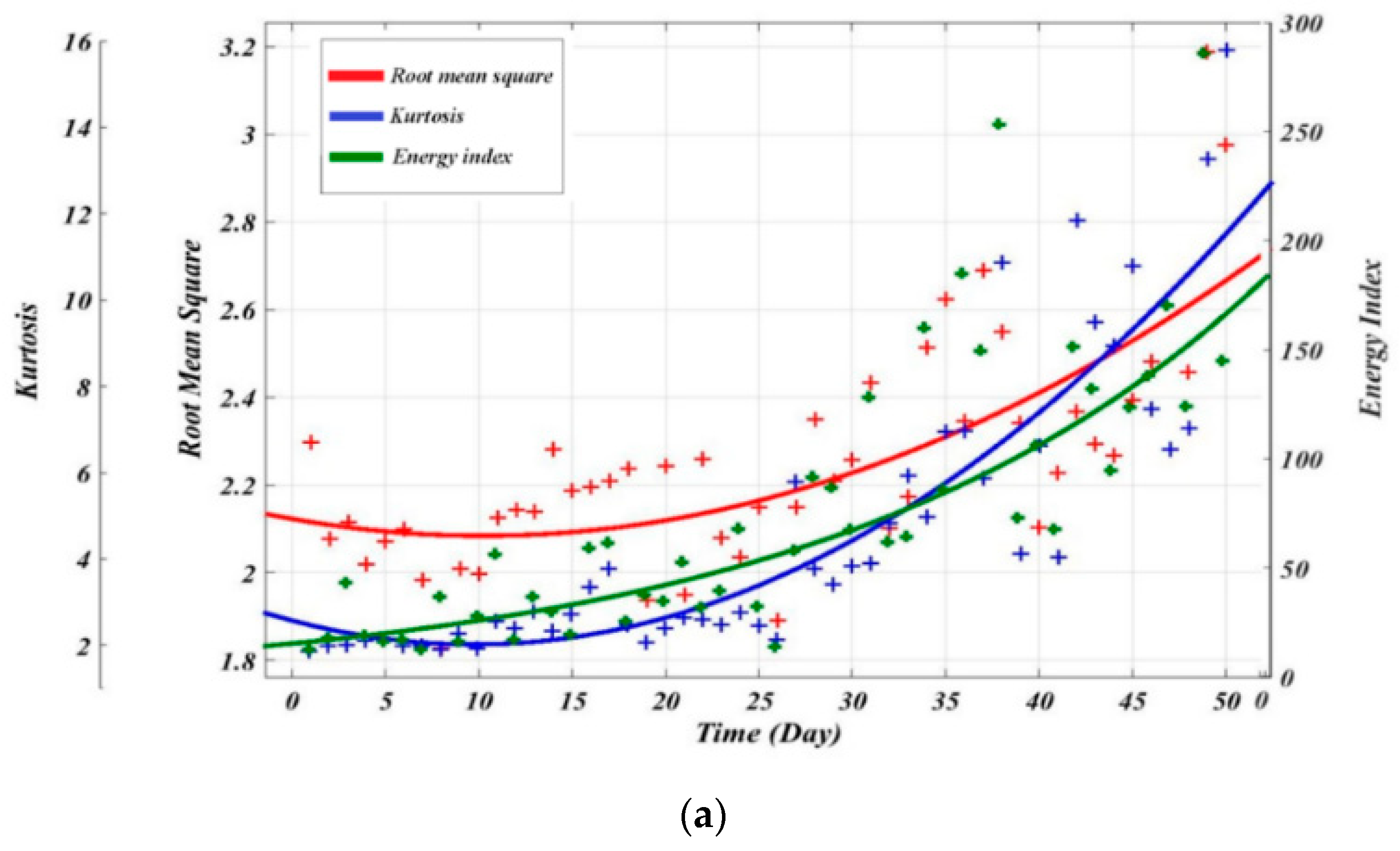
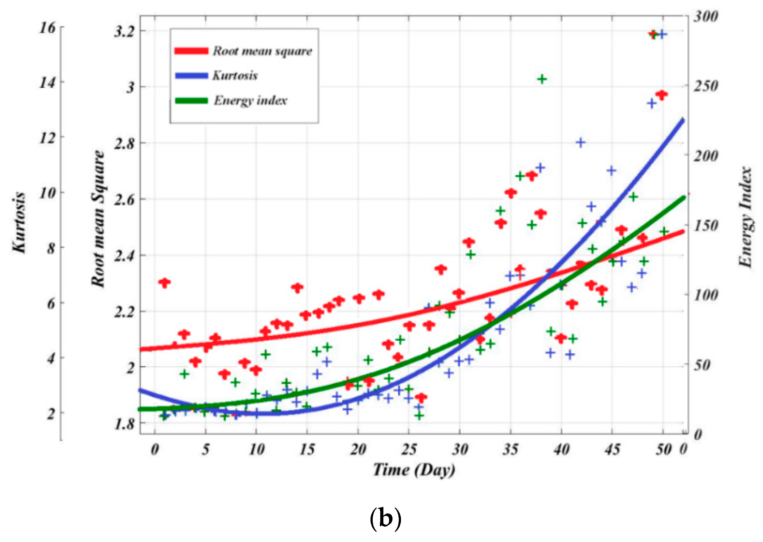
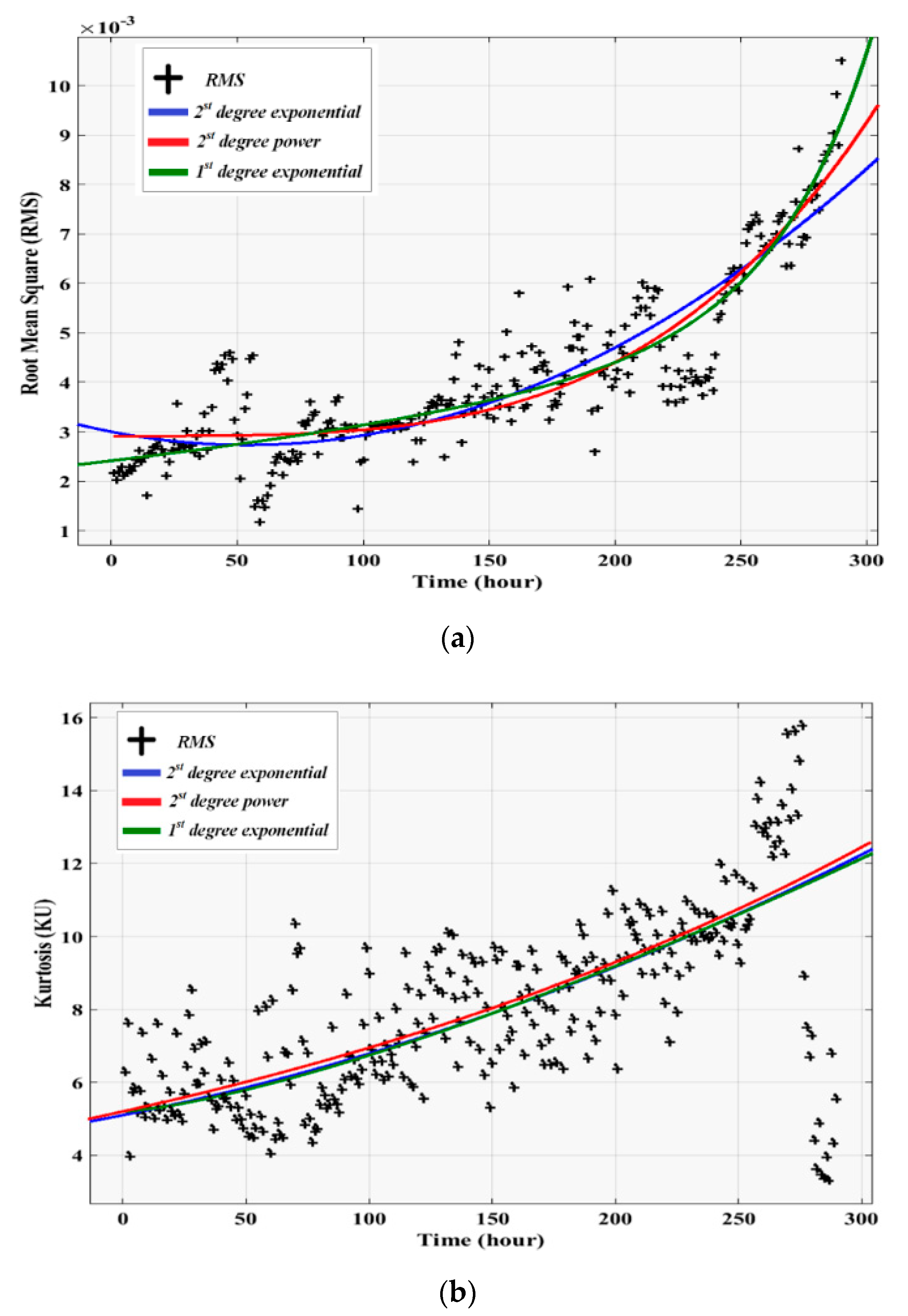
It has been mentioned previously that due to measurement noise, variation of operational conditions and the stochastic nature of the degradation processes, the raw condition indicators cannot be directly used as the inputs of the prediction models. To solve this problem, the obtained raw data were fitted by means of appropriate mathematical functions (i.e., exponential and polynomial models were utilized to represent trends of the condition indicators). The regression model utilized the two equations mentioned above (i.e., Equations (4) and (5)) to find the relationship between condition indicators and time. Figure 7 and Figure 8 show the actual and fitted values of the (a) high-speed shaft bearing case for 50 days of measurements of RMS and KU; and (b) the split cylindrical roller bearing for 298 h of testing.
Table 3 and Table 4 list the optimal fitting parameters and the associated RMSE and adjusted R 2 values for the exponential and polynomial models, respectively. It can be observed that using the exponential regression to fit the condition indicators is more accurate than the polynomial. For instance, in Table 3 RMS showed the lowest value of root mean square error of 0.05248 and a high adjusted R2 with 0.957. Whereas the results obtained from polynomial for the same condition indicator showed the lowest adjusted R2 with 0.5947. Therefore, exponential regression was selected to calculate the RUL, and the computed results were compared to those of the ANN model.

7.2. Artificial Neural Network

In this study, we propose use of an ANN model for estimating the RUL for bearing running at high speed and constant load. The model is a feed-forward back-propagation artificial neural network model with one input layer, a changeable number of hidden layers and one output layer. The optimal number of hidden layers, learning rate and algorithm type were determined during the training process by minimizing the error between target outputs and model outputs. Based on the training results, the ANN model that was finally adopted consisted of one input layer with two inputs, namely raw RMS and KU; one output layer with one output (fitted RMS values); and two hidden layers with 9 neurons in the first layer and 7 neurons in the second layer. The neural network was trained with the resilient back-propagation algorithm and the logistic activation sigmoid function.
The inputs of the ANN model are the raw RMS and KU values, while the target is the best fitted RMS obtained using fitting tools for the same parameter settings. The network structure maps between these variables to generate the function of explaining their relationship. The extracted raw RMS and KU were fed to the model, and the model was trained using the algorithms stated previously. As mentioned previously, the lowest training errors were obtained by an ANN model containing one input layer, one output layer and two hidden layers. The layer size was determined according to the mean square errors between the target output series and the estimated outputs.
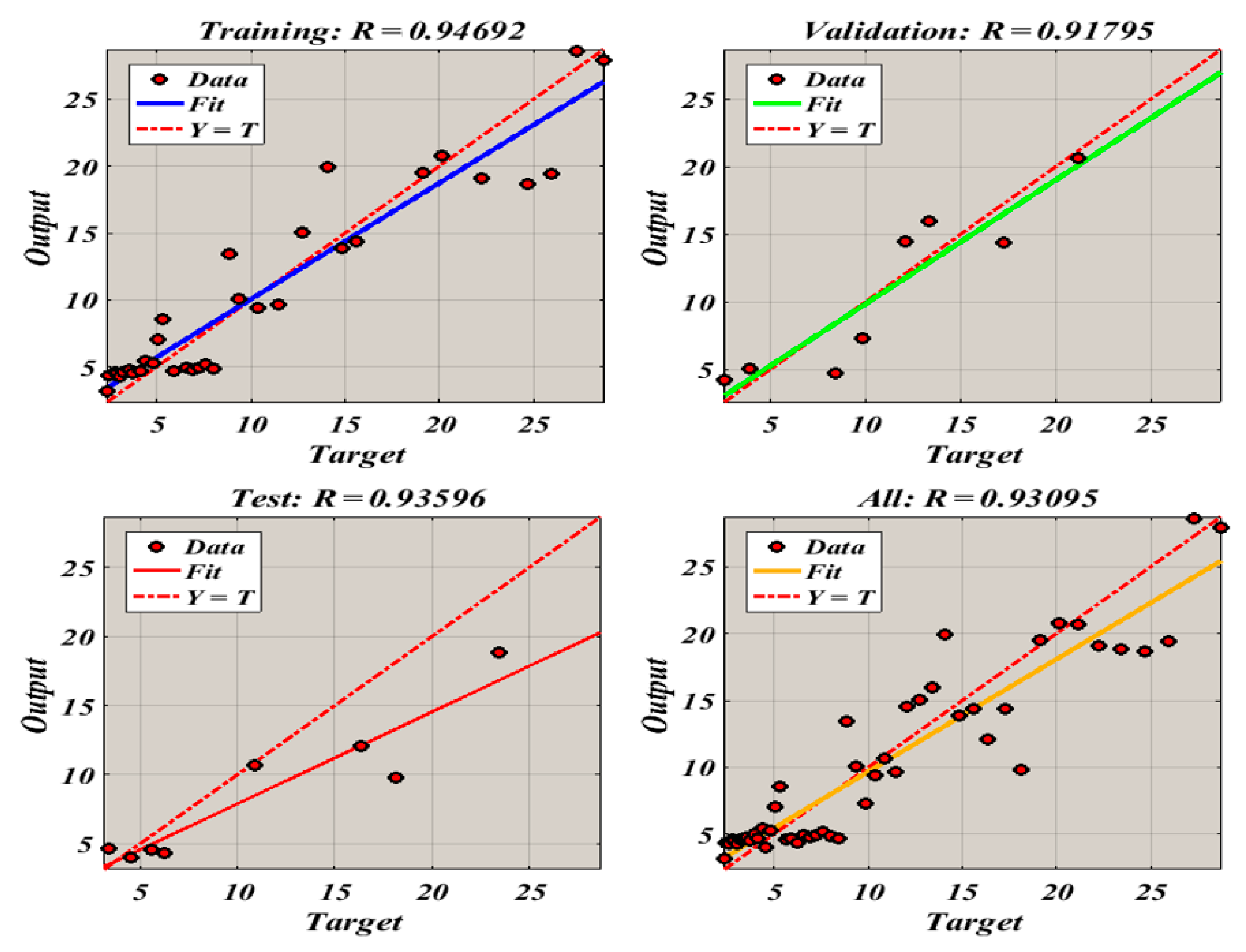
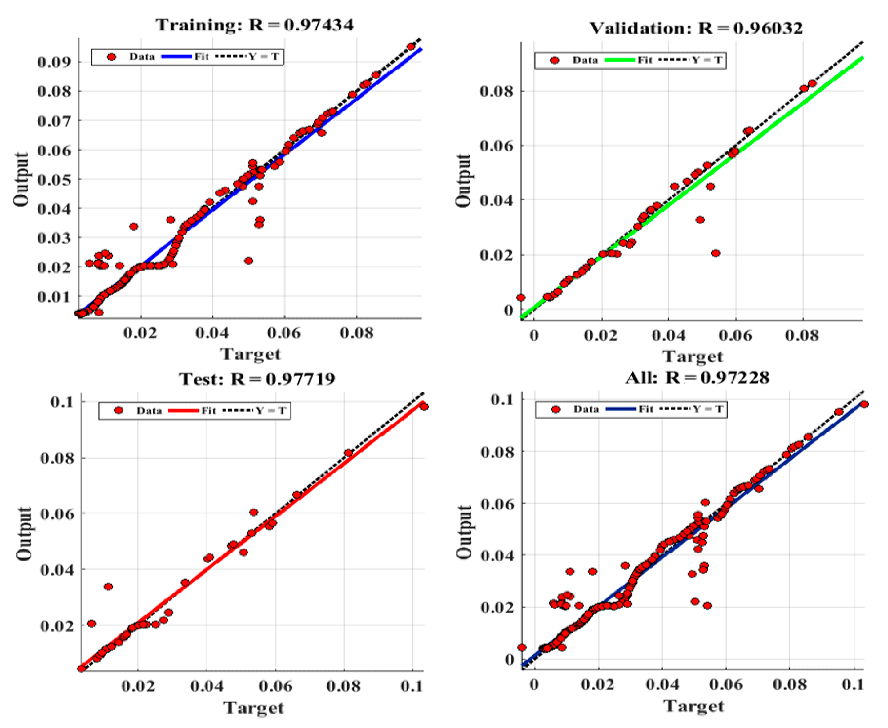
The next phase comprised of validation of the trained model. This was achieved by passing the raw KU and RMS values to the trained model. The ANN model’s output (i.e., estimated fitted RMS) is then extrapolated to a pre-defined failure threshold to predict the RUL of the system. Figure 9 and Figure 10 presented the final results of model output obtained from 70% of training and 30% of testing data. The error and the RUL were calculated using the following equations:
E r r o r   ( % ) =   A c t u a l   ( R U L ) E s t i m a t e d   ( R U L ) A c t u a l   ( R U L )  
R U L   = t f   t c
where t f is the time at which the failure occurred; in this study, t f was chosen as the last time instance of running. The t c is the time point at which the RUL is predicted.
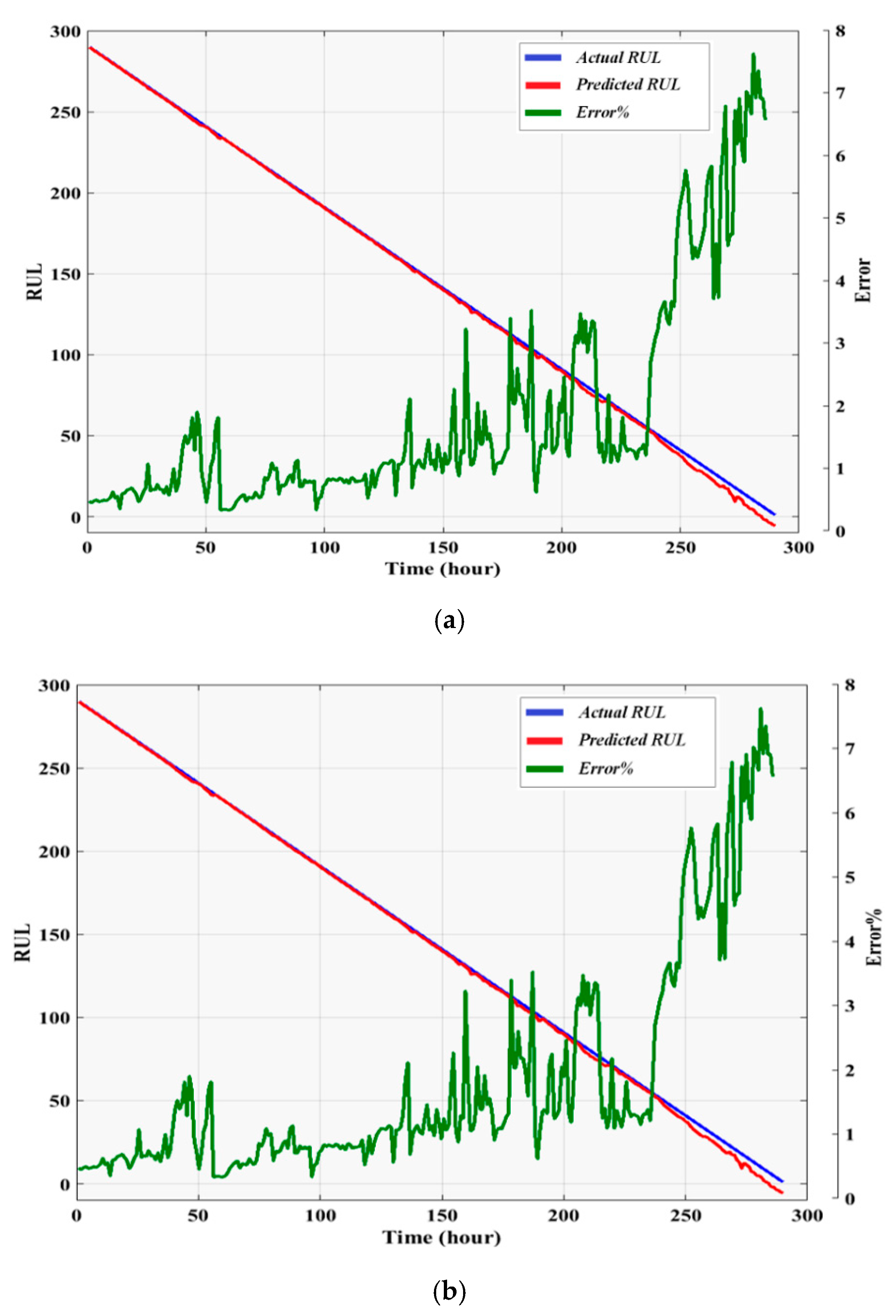
Figure 11 and Figure 12 show the results in terms of RUL prediction. The associated errors are also plotted in the figures. Based on observation of the trends of the predicted RUL compared to the actual one, it is evident that the proposed approach satisfactorily follows the deterioration trend of the bearings under study with small errors. To be specific, Figure 11a depicts the estimated RUL with the actual bearing life using the exponential regression model as a predicted tool. It shows that the trend at the beginning of the prediction initially closely estimated the actual values. However, as the end of bearing life approaches, the prediction deviates from the actual values and oscillates away. Results obtained from the ANN analysis using two inputs (RMS and KU) are depicted in Figure 11b. Results observation shows that the prediction made by the proposed model is very accurate. The RUL results obtained for dataset 2 show that the errors between the 0 and 250 operating hours of the ANN model are significantly lower than those of the regression model. The mean square error (MSE) was calculated in order to further compare the ANN and the regression models. The MSE of the regression model was 14.57, whereas the ANN model only had an MES value of 6.78. Therefore, the prediction made by the proposed ANN model is more accurate.

8. Conclusions

A data-driven prognostics model has been developed for RUL prediction of rolling element bearings. Two types of prediction methods have been used to model and estimate the remnant life: regression and back-propagation neural network. The outputs of the regression model have been used to feed the neural network. This paper explores the possibility of combining regression models with ANNs to improve the predictive accuracy of regression models. This paper also contributes to the existing literature by designing a test rig and conducting experimental tests to generate bearing failure data in order to validate the proposed prognostic model. The model was also validated through industrial data provided by a commercial company.
The obtained results using regression and ANN models have been compared. The performance of each regression model was compared using two parameters: RMSE and adjusted- R 2 . The result showed that the exponential model had better performance than polynomial regression. The results from the proposed ANN show that the model had good performance in predicting RUL of the bearing failure, and this success can be attributed to the link created between the regression model to the ANN through the best fit condition indicator. Comparing performance of the regression model and the ANN, it can be seen that the ANN has better performance; however, this performance cannot be achieved without the regression model, and so therefore the regression model is considered necessary to improve the performance of the ANN model.

Author Contributions

methodology, F.E. and S.S.; writing—original draft preparation, S.S.; writing—review and editing, X.L.; supervision, D.M.

Funding

This research received no external funding.

Conflicts of Interest

The authors declare no conflict of interest.

References

  1. Saha, B.; Goebel, K.; Poll, S.; Christophersen, J. Prognostics Methods for Battery Health Monitoring Using a Bayesian Framework. IEEE Trans. Instrum. Meas. 2009, 58, 291–296. [Google Scholar] [CrossRef]
  2. Misra, K.B. Maintenance Enginerring and Maintenability: An Introduction; Springer: London, UK, 2008. [Google Scholar]
  3. Tondon, N.; Choudhury, A. A review of vibration and acoustics measurement methods for the detection of defects in rolling element bearing. Tribol. Int. 1999, 32, 469–480. [Google Scholar] [CrossRef]
  4. Okoh, C.; Roy, R.; Mehnen, J.; Redding, L. Overview of Remaining Useful Life prediction techniques in Through-life Engineering Services. Procedia CIRP 2014, 16, 158–163. [Google Scholar] [CrossRef]
  5. Li, N.; Lei, Y.; LiN, J.; Ding, S.X. An Improved Exponential Model for Predicting Remaining Useful Life of Rolling Element Bearings. IEEE Trans. Ind. Electron. 2015, 62, 7762–7773. [Google Scholar] [CrossRef]
  6. Wu, J.; Wu, C.; Cao, S.; Or, S.W.; Deng, C.; Shao, X. Degradation Data-Driven Time-To-Failure Prognostics Approach for Rolling Element Bearings in Electrical Machines. IEEE Trans. Ind. Electron. 2018, 66, 529–539. [Google Scholar] [CrossRef]
  7. Sutrisno, E.; Oh, H.; Vasan, A.S.S.; Pecht, M. Estimation of remaining useful life of ball bearings using data driven methodologies. In Proceedings of the 2012 IEEE Conference on Prognostics and Health Management, Denver, CO, USA, 18–21 June 2012; Volume 2, pp. 1–7. [Google Scholar]
  8. Goebel, K.; Saha, B.; Saxena, A. A comparison of three data-driven techniques for prognostics. In Proceedings of the 62nd Society for Machinery Failure Prevention Technology, Virginia Beach, VA, USA, 6–8 June 2008; pp. 1–13. [Google Scholar]
  9. Loukopoulos, P.; Zolkiewski, G.; Bennett, I.; Sampatha, S.; Pilidis, P.; Li, X.; Mba, D. Abrupt fault remaining useful life estimation using measurements from a reciprocating compressor valve failure. Mech. Syst. Signal Process. 2019, 121, 359–372. [Google Scholar] [CrossRef]
  10. Kim, H.-E.; Andy, C.C.; Mathew, J.; Eric, Y.H.; Choi, B.-K. Machine Prognostics Based on Health State Estimation Using Svm. In Proceedings of the Third World Congress on Engineering Asset Management and Intelligent Maintenance Systems Conference, Beijing, China, 27–30 October 2008; pp. 834–845. [Google Scholar]
  11. Zhang, S.; Ganesan, R.; Xistris, G.D. Self-organising neural networks for automated machinery monitoring systems. Mech. Syst. Signal Process. 1996, 10, 517–532. [Google Scholar] [CrossRef]
  12. Mandal, D.; Pal, S.K.; Saha, P. Modeling of electrical discharge machining process using back propagation neural network and multi-objective optimization using non-dominating sorting genetic algorithm-II. J. Mater. Process. Technol. 2007, 186, 154–162. [Google Scholar] [CrossRef]
  13. Elasha, F.; Mba, D.; Togneri, M.; Master, I.; Teixeira, J.A. A hybrid prognostic methodology for tidal turbine gearboxes. Renew. Energy 2017, 114, 1051–1061. [Google Scholar] [CrossRef]
  14. Li, X.; Duan, F.; Loukopoulos, P.; Bennett, I.; Mba, D. Canonical variable analysis and long short-term memory for fault diagnosis and performance estimation of a centrifugal compressor. Control Eng. Pract. 2018, 72, 177–191. [Google Scholar] [CrossRef]
  15. Cheng, F.; Qu, L.; Qiao, W. Fault Prognosis and Remaining Useful Life Prediction of Wind Turbine Gearboxes Using Current Signal Analysis. IEEE Trans. Sustain. Energy 2018, 9, 157–167. [Google Scholar] [CrossRef]
  16. Elforjani, M.; Shanbr, S. Prognosis of Bearing Acoustic Emission Signals Using Supervised Machine Learning. IEEE Trans. Ind. Electron. 2017, 0046, 5864–5871. [Google Scholar] [CrossRef]
  17. Heng, R.B.W.; Nor, M.J.M. Statistical analysis of sound and vibration signals for monitoring rolling element bearing condition. Appl. Acoust. 2002, 53, 211–226. [Google Scholar] [CrossRef]
  18. Zhu, J.; Nostrand, T.; Spiegel, C.; Morton, B. Survey of Condition Indicators for Condition Monitoring Systems. In Proceedings of the Annual Conference of the Prognostics and Health Management Society, Fort Worth, TX, USA, 29 September–2 October 2014; Volume 5, pp. 1–13. [Google Scholar]
  19. Eftekharnejad, B.; Carrasco, M.R.; Charnley, B.; Mba, D. The application of spectral kurtosis on Acoustic Emission and vibrations from a defective bearing. Mech. Syst. Signal Process. 2011, 25, 266–284. [Google Scholar] [CrossRef] [Green Version]
  20. Wang, L.; Gao, R.X. Condition Monitoring and Control for Intelligent Manufacturing; Springer: London, UK, 2006. [Google Scholar]
  21. Bates, D.M.; Watts, D.G. Nonlinear Regression Analysis; Wiley: New York, NY, USA, 2007; 392p. [Google Scholar]
  22. Mahamad, A.K.; Saon, S.; Hiyama, T. Predicting remaining useful life of rotating machinery based artificial neural network. Comput. Math. Appl. 2010, 60, 1078–1087. [Google Scholar] [CrossRef] [Green Version]
  23. Levenberg, K.; Arsenal, F. A Method for the Solution of Certain Non-Linear Problems in Least Squares. Q. Appl. Math. 1943, 1, 536–538. [Google Scholar] [CrossRef]
  24. Bechhoefer, E.; van Hecke, B.; He, D. Processing for Improved Spectral Analysis. In Proceedings of the Annual Conference of Prognostics and Health Management Society, New Orleans, LU, USA, 14–17 October 2013; pp. 1–6. [Google Scholar]
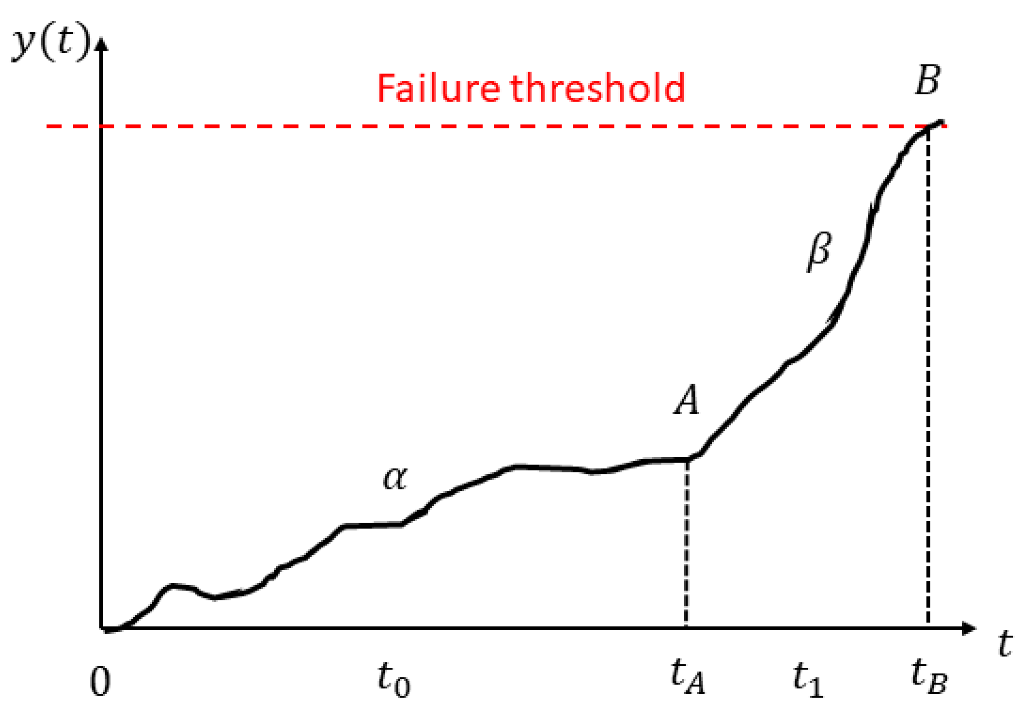
Figure 1. Bearing life process.
Energies 12 02705 g001
Figure 2. Schematic of Regression Process.
Energies 12 02705 g002
Figure 3. Multiple-layer neural network.
Energies 12 02705 g003
Figure 4. Schematic of test rig construction.
Energies 12 02705 g004
Figure 5. Specimen as an assembled and in parts.
Energies 12 02705 g005
Figure 6. Loading system.
Energies 12 02705 g006
Figure 7. Fitted condition indicators for dataset 1: (a) Fitted condition indicators using exponential functions; (b) Fitted condition indicators using polynomial functions.
Energies 12 02705 g007aEnergies 12 02705 g007b
Figure 8. Fitted condition indicators for dataset 2 (exponential and polynomial functions): (a) Actual and fitted root mean square (RMS); (b) Actual and fitted Kurtosis (KU).
Energies 12 02705 g008
Figure 9. Neural Network Training Regression (dataset 1).
Energies 12 02705 g009
Figure 10. Neural Network Training Regression (dataset 2).
Energies 12 02705 g010
Figure 11. Remaining useful life (RUL) results (dataset 1): (a) Regression Model RUL results; (b) Artificial neural network RUL results.
Energies 12 02705 g011
Figure 12. Remaining useful life (RUL) results (dataset 2): (a) Regression Model RUL results; (b) Artificial neural network RUL results.
Energies 12 02705 g012
Table 1. Wind turbine operating details.
Machine StateIncreasing Inner Race Bearing Fault
Power rating 2 MW flux
Nominal speed1800 rpm
Measurement ChannelSensor
Sample rate 97,656 Hz
Record length 6 s
Sensor typeAccelerometer
Table 2. Specification of Cooper cylindrical roller bearing type (01B 40MM GR).
ParameterMeasurement
External Diameter (Pitch)84.14 mm
Internal Diameter (Bore)40.00 mm
Pitch Circle Diameter62.71 mm
Roller Diameter11.91 mm
Number of Rollers10
Weight of the Specimen1.2 kg
Table 3. Optimal estimated exponential model constants.
Condition IndicatorsDataset 1Dataset 2
Model ConstantsRMSEAdj. R2Model ConstantsRMSEAdj. R2
abab
RMS2.2350.05110.052480.9570.0038350.37970.0007170.995
KU3.4390.11210.94690.9757.870.25480.24940.990
Table 4. Optimal estimated polynomial model constants.
Condition IndicatorsDataset 1Dataset 2
Model ConstantsRMSEAdj. R2Model ConstantsRMSEAdj. R2
a0a1a2a0a1a2
RMS2.190.1170.00440.16440.59470.0005520.0013650.0036020.00077350.853
KU3.240.57180.30040.21720.8810.2441.9717.7860.38510.792