Kinetic Evaluation of Lime for Medium-Temperature Desulfurization in Oxy-Fuel Conditions by Dry Sorbent Injection

Abstract

With increasing emphasis on the control of greenhouse gases, power plants may move towards oxy-fuel technologies rather than air-fired plants. This move leads to a change in the feed to the desulfurization unit, which also needs to be adapted along with the power plant. Most existing plants already have functioning desulfurization units, which need to be retrofitted for the new conditions. In the present study, three different limes have been examined as sorbents for sulfur capture in oxy-fuel conditions with varying residence times at medium temperature (150–450 ${}^{\circ }$C). Parameters indicative of the kinetics and competition between SO${}_2$ and CO${}_2$, like SO${}_2$ breakthrough time, total lime conversion, yield for sulfur capture and sulfur selectivity have been evaluated. The results of this study lead to the recommendation that medium temperature desulfurization should be used for moderate SO${}_2$ capture, in combination with already existing sulfur capture systems. The effects of CO${}_2$ and water vapor have also been analyzed. In addition, the performance of the unit irrespective of temperature strongly depends on the lime type. In addition, absence of water vapor strongly favored the desulfurization process when there was high concentration of CO${}_2$.

1. Introduction

Dry sorbent injection (DSI) methods have been studied as a means of desulfurization for a considerable time, with only moderate SO${}_2$ capture achieved. However, they can be retrofitted to already existing power plants, making them attractive from a capital cost point of view in comparison to other flue-gas desulfurization (FGD) systems [1]. A process flow diagram of a typical air-fired power plant is shown in Figure 1 and, as can be seen, it offers temperatures that range from below 100 ${}^{\circ }$C after the air-heater to 1200 ${}^{\circ }$C in the upper furnace [2]. Desulfurization can be performed at different temperatures with varying mechanisms, by injecting the sorbent at different injection points. There are currently a number of working FGD plants based on dry sorbent injection for high temperature desulfurization (usually >600 ${}^{\circ }$C) in the furnace and low temperature desulfurization (usually <150 ${}^{\circ }$C) in the duct system, around the world [1,2,3,4,5,6,7,8,9,10,11,12,13,14,15,16,17,18,19]. However, there are few working plants with lime-injection at medium-temperature in the economizer [1,2].

The possible percentage of SO${}_2$ removal in the medium-temperature economizer is as high as that in the furnace and of that downstream of the air heater, making it an attractive alternative for desulfurization [2]. Fernández et al. have studied the desulfurization of lime between 300–450 ${}^{\circ }$C using Ca(OH)${}_2$ and it was found that in the temperature range, the best performance was at 450 ${}^{\circ }$C, a temperature which is suitable for the economizer injection [20,21]. Desulfurization studies in the range of 50–400 ${}^{\circ }$C can also be found, where SO${}_2$ removal has been shown to be better at 400 ${}^{\circ }$C (economizer temperature) in comparison to other temperatures (duct temperatures) in the range, encouraging further attention to economizer FGD studies [22]. Studies in the temperature range of 120–240 ${}^{\circ }$C, with regenerable CaO-alumina [23], and 60–300 ${}^{\circ }$C, with fly-ash [19], have both been subjects of past research. However, these studies correspond more to the in-duct injection or at best, provide partial input for economizer injection studies at the lower end of the temperature range. Other desulfurization studies provided understanding of the mechanism and the chemistry involved in the medium-temperature process, but lack application-oriented performance or kinetic studies [24,25,26,27].

Another aspect of economizer injection is that the residence time is quite low, about 1–2 s. To facilitate higher residence times, a medium-temperature baghouse, in place of one that operates at low temperatures (in Figure 1, the air heater ensures low temperature in the baghouse), could be used. Recycling the sorbent in addition to using a medium-temperature baghouse, could further enable longer residence times. Another option would be to combine the medium temperature injection with other FGD systems, for example, wet FGD. Using a medium-temperature baghouse might call for repositioning of the air heater in order not to sacrifice the high efficiency of the power plant [28]. On the contrary, it might eliminate the air heater altogether, without losing any efficiency, if there already exists a heat recovery unit downstream, as in some hybrid desulfurization units [1,2]. Li et al. has worked on convective sorbent injection in combination with a medium-temperature baghouse, with promising results. The work refers to the region before the economizer, with super-heater and reheater in Figure 1, in the temperature range of 425–650 ${}^{\circ }$C [29,30,31]. Additionally, operation in the economizer does not mainly lead to formation of CaO but instead leads to SO${}_2$ reacting with the lime [2]. Therefore, the studies by Li et al. are insufficient to explore the potential for desulfurization in the economizer in combination with a medium-temperature baghouse, where the decomposition of lime to CaO does not take place.

The aforementioned research was all based on air-fired plants. In an attempt to decrease the greenhouse gases, especially CO${}_2$, research has tended to focus on oxy-fired power plants, among other things. Such plants have an exhaust gas stream concentrated in CO${}_2$. Changing the feed to the power plant and thus also the feed to the desulfurization system, calls for desulfurization units that are adapted to the new feed concentrated in CO${}_2$. Very few studies were found on oxy-fuel desulfurization [4,32,33]. Stewart et al. and Chen et al. have studied high-temperature desulfurization using limestone as sorbent in oxy-fuel conditions. At high temperatures, the reaction proceeds via CaO formed by decomposition of the carbonate or directly via the carbonate. These studies show that the presence of CO${}_2$ retards the pathway through formation of CaO but positively affects the pathway through CaCO${}_3$, in the high temperature range. They further show that the approach for desulfurization needs to shift towards providing higher residence times, as the slower reaction mechanism which goes through carbonation of the lime, is favored in the presence of high CO${}_2$ [4,32]. Moreover, Li et al. observed that injection above 500 ${}^{\circ }$C led to much higher carbonation levels with only 14% CO${}_2$ in the inlet stream [29,30,31]. This observation also strongly supports the previous argument that the pathway via CaCO${}_3$ might be favored by oxy-fuel conditions, where the CO${}_2$ concentration is much higher. This emphasizes the need to study the effect of high CO${}_2$ in the case of medium-temperature injections as well, preferably with high residence times.

In addition, in the case of air-fired plants, the formation of CaO by dehydration of lime is an important step to expose the unreacted Ca(OH)${}_2$ or CaO surfaces to SO${}_2$ owing to the mechanism involved, which goes through sulfation of CaO or Ca(OH)${}_2$ [2]. As mentioned earlier for the case of high temperature, in the presence of high concentrations of CO${}_2$, as in the case of oxy-fired plants, the reaction does not go through formation of CaO, instead it goes through CaCO${}_3$ [4,32]. However, the necessity of reactive CaO in case of medium temperature oxy-fuel desulfurization is yet to be evaluated. Wang et al. have previously studied medium-temperature desulfurization of lime in oxy-fuel conditions, avoiding dehydrating conditions, with encouraging results like lime consumption as high as 76% [33]. The work introduces implementation of medium-temperature desulfurization in an oxy-fired power plant and discusses its performance, but lacks a detailed kinetic evaluation of the medium-temperature desulfurization process. Kinetics are an important consideration in the design of the desulfurization unit of a power plant and henceforth will be the subject of the present study. Kinetic parameters like SO${}_2$ breakthrough time, total lime conversion, sulfur yield and sulfur selectivity are chosen as performance indicators.

This work, therefore, focuses on the evaluation of kinetics in relation to the following aspects:

• Medium temperature dry lime (Ca(OH)${}_2$) injection in the economizer;
• Temperatures below 450 ${}^{\circ }$C, where decomposition of lime does not take place;
• Mainly oxy-fuel conditions (60% CO${}_2$) with some air-fired (10% CO${}_2$) experiments for comparison;
• Effect of residence time, which would determine the degree of changes required in order to retrofit a plant with the new FGD unit.
• Effect of water vapor.
• Type of lime.

The temperature range was fixed between 150–450 ${}^{\circ }$C. Lower temperatures (150–300 ${}^{\circ }$C) were studied to facilitate the understanding of the reason behind the change in performance due to the presence of CO${}_2$. The effect of water vapor and CO${}_2$ in the feed stream is examined as well. This work builds on the previous study [33] on oxyfuel combustion and regenerative calcium cycle. In this process lime absorbs CO${}_2$ in the flue gas and be converted to calcium carbonate, which is separated and transferred to the calciner. In the calciner, calcium carbonate is converted to calcium oxide, which returns to the carbonator for CO${}_2$ capture. In the presence of SO${}_2$ the lime will also adsorb SO${}_2$ in the flue gas. This leads to deactivation in the system and the requirements for solids recirculation increase. This necessitates the need for investigating desulfurization at high CO${}_2$ concentration. However, this paper differs from [33] in that the medium-temperature injection is evaluated from a kinetics point of view as opposed to a purely process point of view. Further, note that lime in this study refers to Ca(OH)${}_2$. CaO is referred to as dehydrated lime.

2. Method

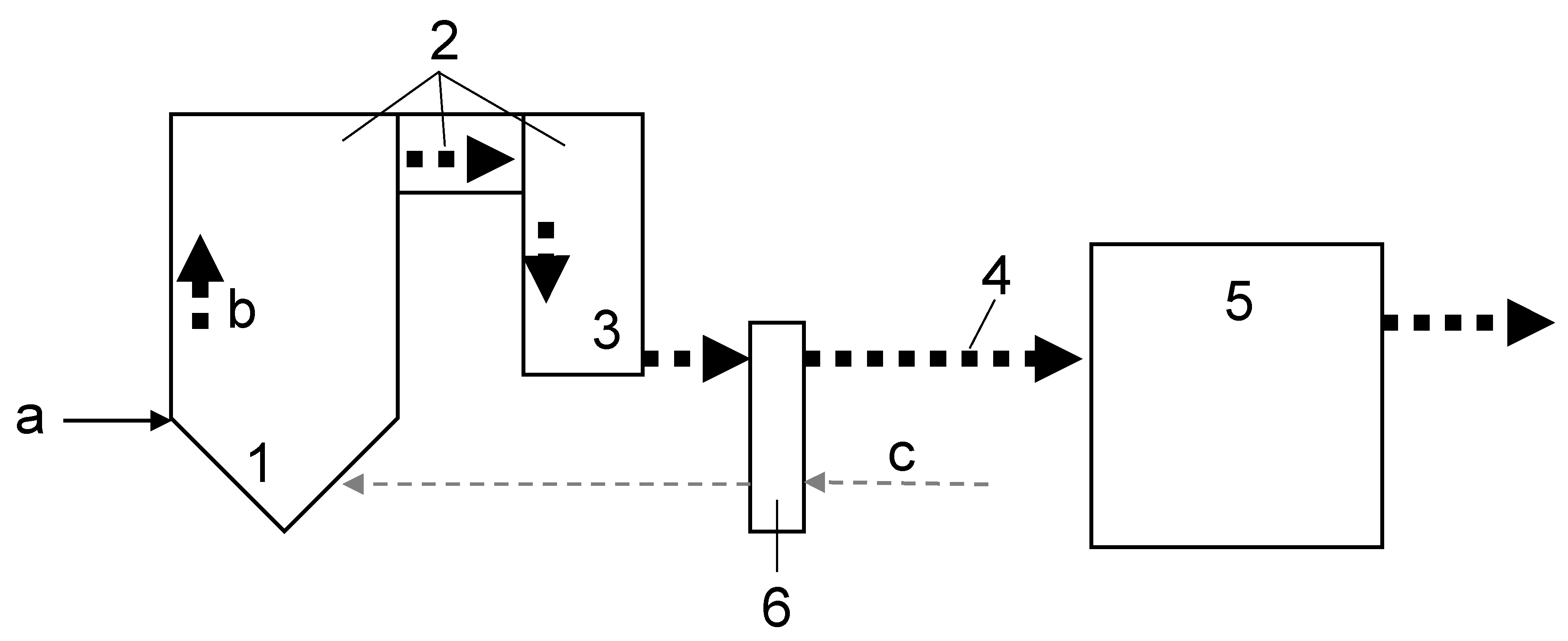
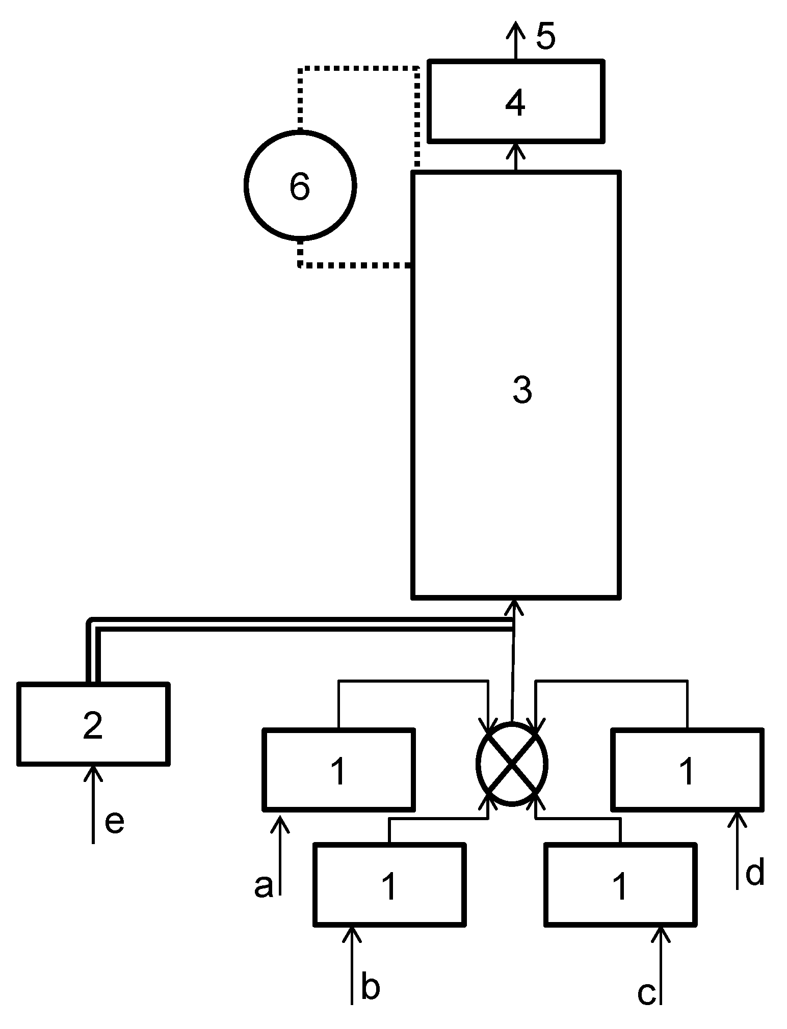
2.1. Experimental Setup for Continuous Runs

The experimental setup for the continuous experiments is shown in Figure 2. The gases used in the experiments were mixed by controlling the mass flow of each of the gaseous compounds. Water was added using a syringe and then heated to produce water vapor. The total flow rate was kept at 500 NmL/min for all experiments. A glass reactor (3.4 cm in external diameter) was filled with a mixture of 1 g of lime and 40 g of sand. The temperature of the reactor was maintained constant using a feedback control from a thermocouple attached to the outer wall of the reactor, to control the heater that maintained the reactor temperature. Dehydration of the lime was avoided by ensuring required flow of water vapor before heating the reactor to the required temperature. The exhaust gas was analyzed using an Emerson built Rosemount NGA 2 000 MLT 4T or a Hiden Analytical HPR-20 mass spectrometer (MS). The experimental setup has been described in more detail in [33]. At the end of the experiments, the total sulfur and carbon content were analyzed using a LECO CS230SH sulfur and carbon analyzer. The flow conditions, reactor dimensions and dilution factors were chosen to minimize heat and mass transfer limitations that are not process intrinsic. Wall effects, dilution effects and axial dispersion were also taken into consideration in the reactor design as per [34].

2.2. Experimental Conditions for Continuous Runs

Experiments were conducted mainly by changing the temperature between 150–450 ${}^{\circ }$C with lime A and base-case conditions. The base-case conditions refer to the experimental conditions that were prevalent in most of the runs, which were 2000 ppm of SO${}_2$, 60% CO${}_2$, 25% H${}_2$O, 2.5% O${}_2$ and the rest being inert (N${}_2$ or Ar). These values represent typical conditions for oxyfuel conditions. The limes were then varied between lime A, lime B and lime C for some temperatures. Properties of the three lime types are shown in

Table 1. Properties of the slaked limes investigated.

	Lime A	Lime B	Lime C
	Standard Type	Sorbacal SP *	Sorbacal SPS *
Species/Property		Weight Percent
Ca(OH)${}_2$	85.1	85.4	85.5
CaCO${}_3$	3.8	8.5	8.7
Inert	11.1	6.1	5.8
Surface area (m${}^2$/g)	17	44	43
Pore volume (mL/g)	0.08	0.23	0.21
Pore diameter $d_{50}$ (nm)	19	22	20

* https://www.sorbacal.com.

. Pore volumes and surface areas were determined using a Micromeritics ASAP 2400 instrument. The intention was to compare standard type Lime A with a so-called enhanced lime (Sorbacal SP) and one activated and enhanced lime (Sorbacal SPS).

Two types of experiments were conducted: short-term and long-term. Short-term experiments produced screening data to study the impact of different parameters. Long-term experiments uncovers information on reactivity decay and how the composition of the reacted limes change with exposure time. The short-term experiments were all run for about 0.8–2.5 h (

Table 2. Experimental conditions for the base-case, short term experiments.

Lime Type	Temperature (${}^{\circ }$C)	Time (h)
Lime A	450	2.0
	350	1.3	1.0 *
	300	2.2
	250	0.8	0.8 *
	200	1.2	1.0 *
	150	1.2
Lime B	450	2.0
	350	2.0	1.5 *
	250	2.0
	200	4.0
Lime C	450	1.8
	350	2.0
	250	2.5
	200	1.8

* Double experiments to check repeatability.

) for base-case conditions, except one experiment with lime B at 200 ${}^{\circ }$C that was accidentally run for 4 h. Based on the results of short-term experiments for lime A, two temperatures were chosen to test the long-term behavior of all the limes by running 12 h experiments. The long-term experiments were conducted for 12 h in all cases. The varying parameters for the base-case, short-term experiments are listed in Table 2. Some of the experiments were also repeated to check the repeatability of the results. The repeatability was tested in the measurement of the breakthrough time, but the total sulfur and carbon analysis was not performed on these samples. These experiments are marked in Table 2.

The influence of CO${}_2$ on the lime performance for sulfur capture was tested by lowering the CO${}_2$ concentration to 10% and 0%, simultaneously increasing the inert concentration to keep the total flow at 500 NmL/min. The experimental conditions for these runs are mentioned in

Table 3. Additional experiments conducted to test the effect of CO${}_2$ concentration on the performance of lime A.

Temperature (${}^{\circ }$C)	CO${}_2$ Concentration (%)	Time (h)
450	10	2.5
	0	3.5 *
350	10	1.8
	0	1.7
150	10	5.5

* The experiment was terminated with only 84% SO${}_2$ breakthrough.

. Unless otherwise mentioned, the experimental conditions are the same as in the base-case runs. For example, in Table 3, the water vapor content is not stated, as it is 25%, the same as in base-case experiments. Tests were also run to understand the influence of water vapor by changing the water vapor concentration from 25% to 0% (see

Table 4. Additional experiments conducted to test the effect of water vapor on the performance of lime A. The water vapor content is 0% in all the below mentioned experiments.

Temperature (${}^{\circ }$C)	CO${}_2$ Concentration (%)	Time (h)
450	60	2.2
	0	3.3
350	60	1.8
	0	2.3

for experimental conditions). The experiments with changing CO${}_2$ and H${}_2$O concentrations were limited to lime A. Additionally, some of the experiments had to run for different times as full breakthrough of SO${}_2$ was not observed, with the exception of an experiment at 450 ${}^{\circ }$C with 0% CO${}_2$ that was terminated with 84% SO${}_2$ breakthrough.

2.3. Data Analysis

The SO${}_2$ concentrations obtained from the Emerson built Rosemount NGA 2000 MLT 4T were absolute while the readings from the MS were calibrated to give SO${}_2$ concentrations relative to the inert (Ar) in the system. Since the inert does not react, the concentrations when reduced relative to the inert are also absolute. However, these concentrations showed an error of 10% since the SO${}_2$ in the system was in ppm. To make the results more comparable, the SO${}_2$ breakthrough curves obtained were normalized to the total SO${}_2$ concentration, i.e., to the SO${}_2$ concentration after 100% breakthrough. The breakthrough times required for 10% and 90% of the total SO${}_2$ concentration were obtained from such normalized curves. The 10% breakthrough times are considered as performance indicators to judge the “immediate” reactivity of the limes. The instrumental error was much higher, below 10% SO${}_2$ breakthrough and has therefore been avoided in the analysis.

The total sulfur and carbon analysis was used to further obtain the yield and selectivity for sulfur $(Y_{\left(S{O}_2\right)}$ and $S_{\left(S{O}_2\right)})$, as well as the total conversion of free lime (X). The yields for sulfur and carbon are defined as percentage of converted lime that formed sulfate and carbonate respectively. The total conversion, selectivity and yields are then related as per the equations below in (1). The procedure is described in more detail in [33].

$$S_{\left(C{O}_2\right)}+S_{\left(S{O}_2\right)}=100X=Y_{\left(C{O}_2\right)}+Y_{\left(S{O}_2\right)}Y=S\times X/100$$

(1)

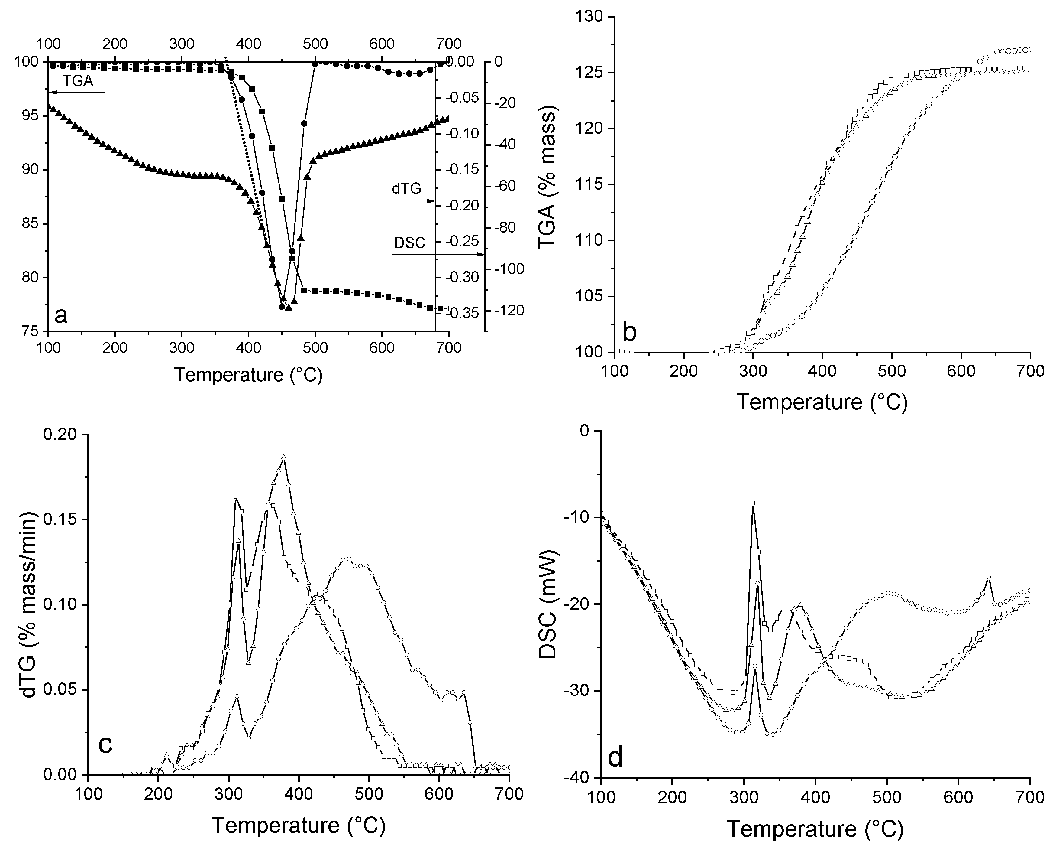
2.4. Thermodynamic Analysis and Characterization

We have previously conducted a thermodynamic analysis to understand which of the species is stable under the experimental conditions [33]. Thermal gravimetric analysis (TGA) and differential scanning calorimetry (DSC) were conducted on lime samples using the Mettler TGA/DSC 1 STARe system. The temperature was increased from 30–900 ${}^{\circ }$C at a rate of 20 ${}^{\circ }$C/min. A flow of 80 mL/min of air or CO${}_2$ was kept over the samples. The procedure for the BET analysis of the various lime samples used was presented earlier [33].

3. Results

In this section, the kinetic performance indicators such as breakthrough times for 10% and 90% SO${}_2$, conversion, selectivity, and yield are presented with the temperature for different types of lime. Furthermore, the results are described with respect to the effect of temperature, CO${}_2$ and H${}_2$O. This discussion facilitates a better understanding of the effect of CO${}_2$, H${}_2$O, temperature, and lime type on the kinetics of the sulfation process. The results correspond to that of base-case concentrations for the experiments conducted to study the effect of temperature. In the case of the effect of CO${}_2$ and H${}_2$O, the parameters that were varied are displayed, and the rest of the conditions correspond to the base-case. The results from thermodynamic analysis and characterization techniques such as BET, TGA and DSC are also explained below.

3.1. Thermodynamics and Characterization

A thermodynamic analysis of the system showed that under the experimental conditions (i.e., with 25% H${}_2$O and under 450 ${}^{\circ }$C), Ca(OH)${}_2$ (or lime) is more stable compared to the dehydrated product CaO. This shows that the decomposition of Ca(OH)${}_2$ does not take place under these conditions. For the CO${}_2$ concentrations between 10% and 60% and H${}_2$O concentration of 25%, CaCO${}_3$ is stable in comparison to Ca(OH)${}_2$. However, CaSO${}_4$ is even more favorable when compared to CaCO${}_3$ under the experimental conditions. Even if CaCO${}_3$ forms in the process, thermodynamics predicts that it will react with SO${}_2$ and O${}_2$ to form CaSO${}_4$. Furthermore, the hydrates, CaSO${}_4$·1/2H${}_2$O and CaSO${}_4$·2H${}_2$O, are also not favorable to CaSO${}_4$ [33].

The structural properties of the limes were previously determined using BET analysis, and it was found that lime B and C have a higher surface area (44 and 43 m${}^2$/g respectively) compared to lime A (17 m${}^2$/g). The pore volumes of lime B and C were also found to be higher than that of lime A; 0.23 and 0.21 mL/g for lime B and C to 0.08 mL/g for lime A. On the other hand, the pore diameters were very close to each other (19, 22, 20 nm for lime A, B and C respectively).

TGA for lime A in air, the derivative of TGA (dTG) and the corresponding DSC results are shown in Figure 3a. From the figure, the onset of the dehydration process is found to be around 380 ${}^{\circ }$C. However, the TGA and DSC were performed using atmospheric air, where the water vapor pressure is as low as 0.01–0.05 bars [35]. The dehydration temperature thus obtained is in agreement with the thermodynamic analysis [33] that estimates a dehydration temperature of 340–400 ${}^{\circ }$C in the aforementioned range of water vapor pressure. In their work, Li et al. state the decomposition temperature as 427 ${}^{\circ }$C for 8.17–8.54% H${}_2$O concentrations [29]. This is also in close agreement with the thermodynamics, which estimate that the dehydration temperature is approximately 407–411 ${}^{\circ }$C [33]. In the case of 25% H${}_2$O in the inlet stream, the estimated dehydration temperature is above 450 ${}^{\circ }$C [33].

TGA of the limes with 100% CO${}_2$, showed that carbonation of lime A takes place at around 290 ${}^{\circ }$C whereas carbonation of lime B and C began at 250 ${}^{\circ }$C [33] (also shown in Figure 3b). Additionally, dTG and DSC results in pure CO${}_2$ are compared for all the limes in Figure 3c and Figure 3d, respectively. They both show that the carbonation indeed takes place in two steps. This is seen as a slight change in slope in the TGA (Figure 3b), which is clearly visible as the two peaks in the dTG (Figure 3c). The results from DSC (Figure 3d) are in agreement with the dTG results. Furthermore, both dTG and DSC results show a shift in the maximum of the second carbonation peak for lime A when compared to lime B and C. This is also seen in Figure 3b as the curve for lime A transforms over a larger range of temperature. Such a shift would suggest that carbonation of lime A is lower when compared to lime B and C, at the experimental conditions used. It would be much higher at temperatures higher than 450 ${}^{\circ }$C, i.e., in case of injection before the economizer.

The dTG and DSC results further show that the rate of both carbonation steps is much higher in the case of lime B and C, when compared to lime A. This is clearly visible in the magnitude of the two peaks in both the dTG and DSC curves. The thermodynamic analysis shows that the carbonation is stable for all temperatures under 900 ${}^{\circ }$C when pure CO${}_2$ is used [33]. Nevertheless, Figure 3b,c shows that the kinetics of carbonation are negligible below 200 ${}^{\circ }$C for all limes even if formation of carbonate is thermodynamically preferred at this temperature.

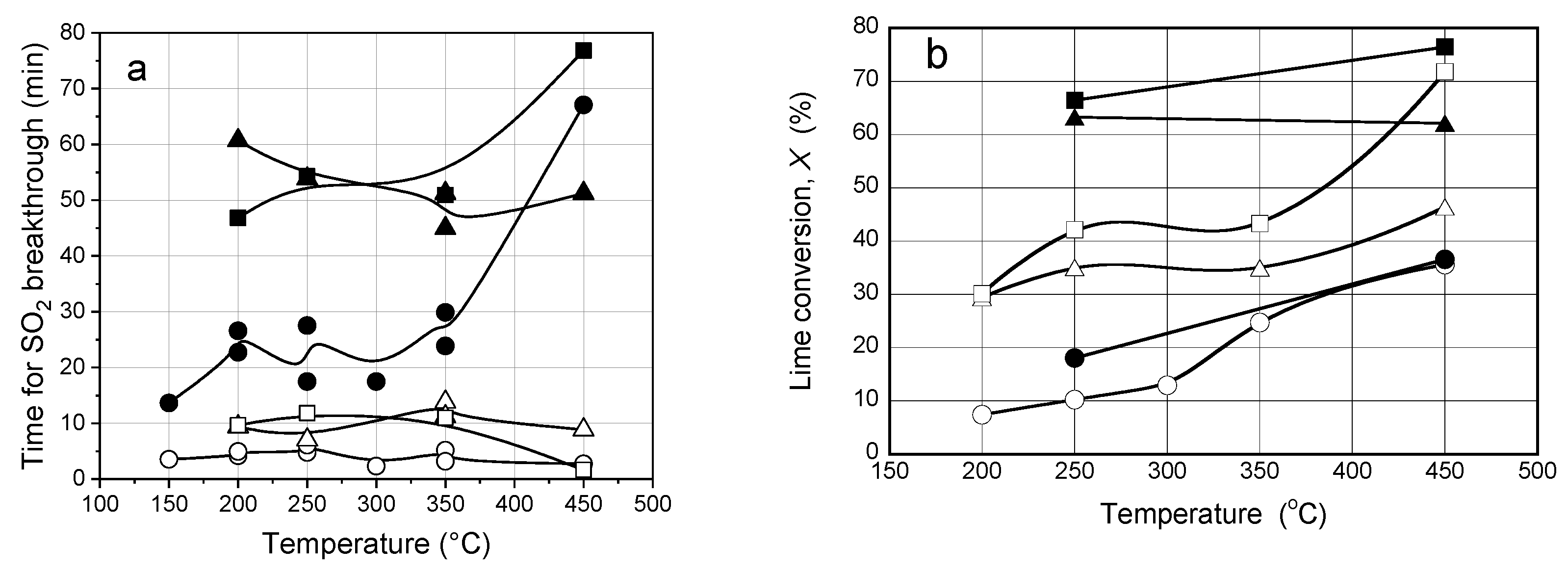
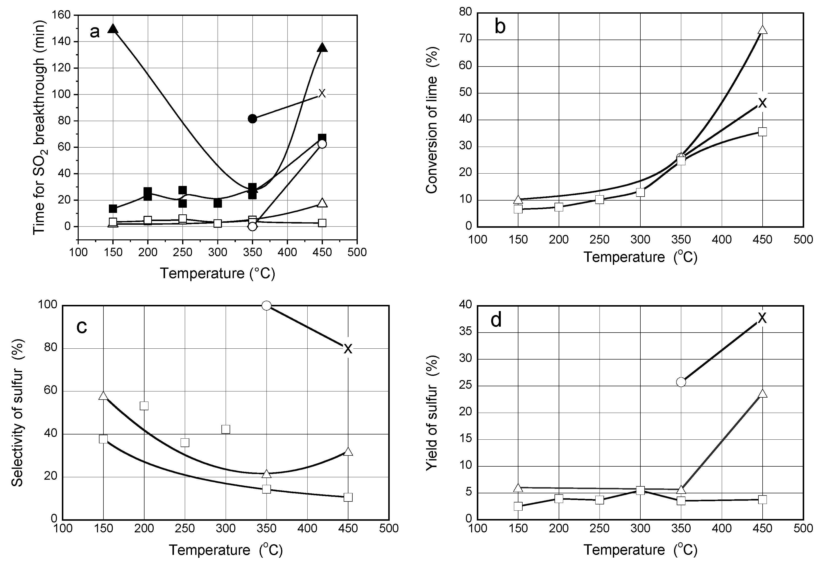
3.2. Continuous Runs—Base-Case Experiments—Effect of Temperature

Figure 4a compares the time taken for the breakthrough of 10% and 90% SO${}_2$ with the temperature for the different limes. The 10% breakthrough times for lime A, B and C have been fairly constant with the temperature, with the exception of lime C at 450 ${}^{\circ }$C, which is much lower than that at other temperatures. In addition, lime B and C clearly have higher 10% SO${}_2$ breakthrough times compared to lime A. The breakthrough time for 10% SO${}_2$ is a measure of how well the SO${}_2$ would be captured if the residence time of lime is very low (about a few minutes) and it can be seen that limes B and C are better for low residence time applications (except lime C at 450 ${}^{\circ }$C). All the 90% SO${}_2$ breakthrough times for lime A are between 10–30 min, except at 450 ${}^{\circ }$C, where they are close to 70 min, much higher than at other temperatures. For lime B, they lay between 45–60 min, about five times higher than 10% SO${}_2$ breakthrough times for the same lime. In contrast to lime A, the 90% SO${}_2$ breakthrough times are fairly constant for lime B. For lime C, the breakthrough times for 90% SO${}_2$ are about 45–55 min for all temperatures except 450 ${}^{\circ }$C, where it is close to 75 min.

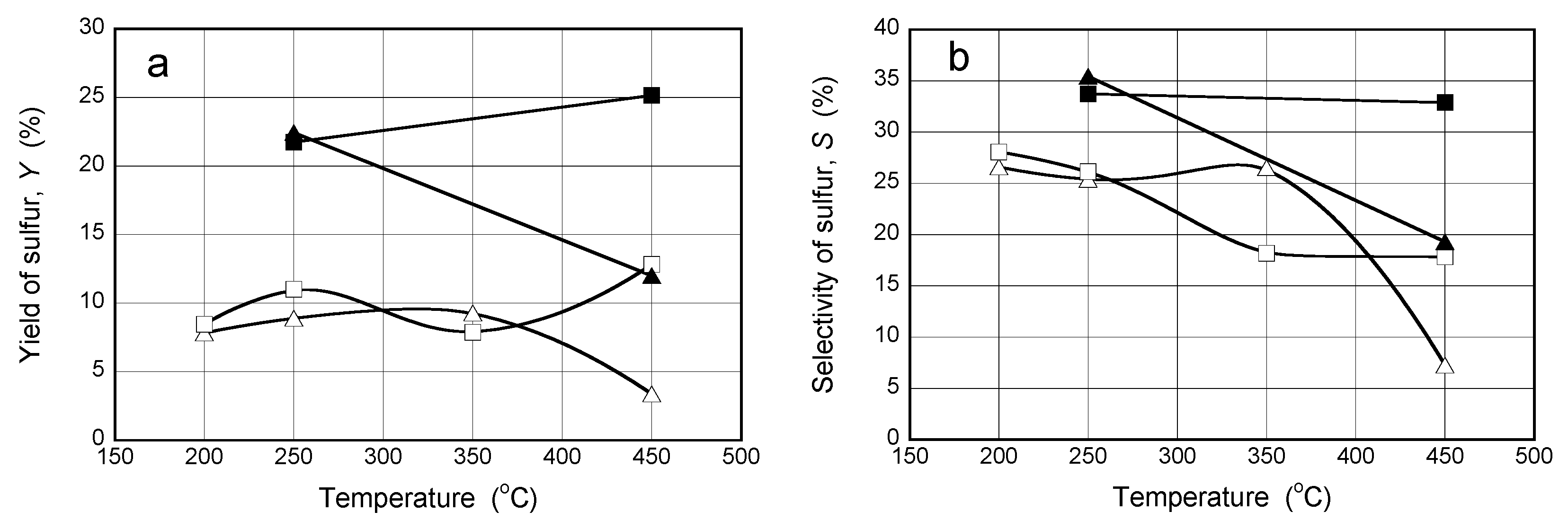
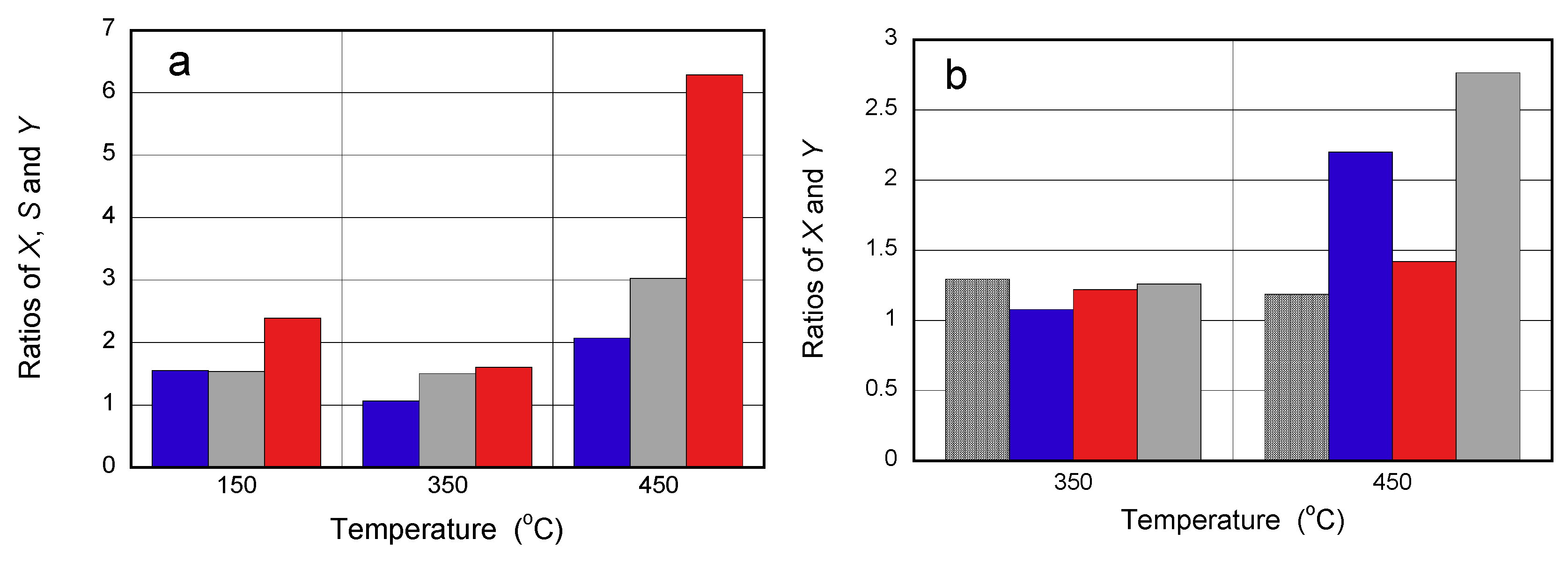
3.3. Conversion, Yield and Selectivity

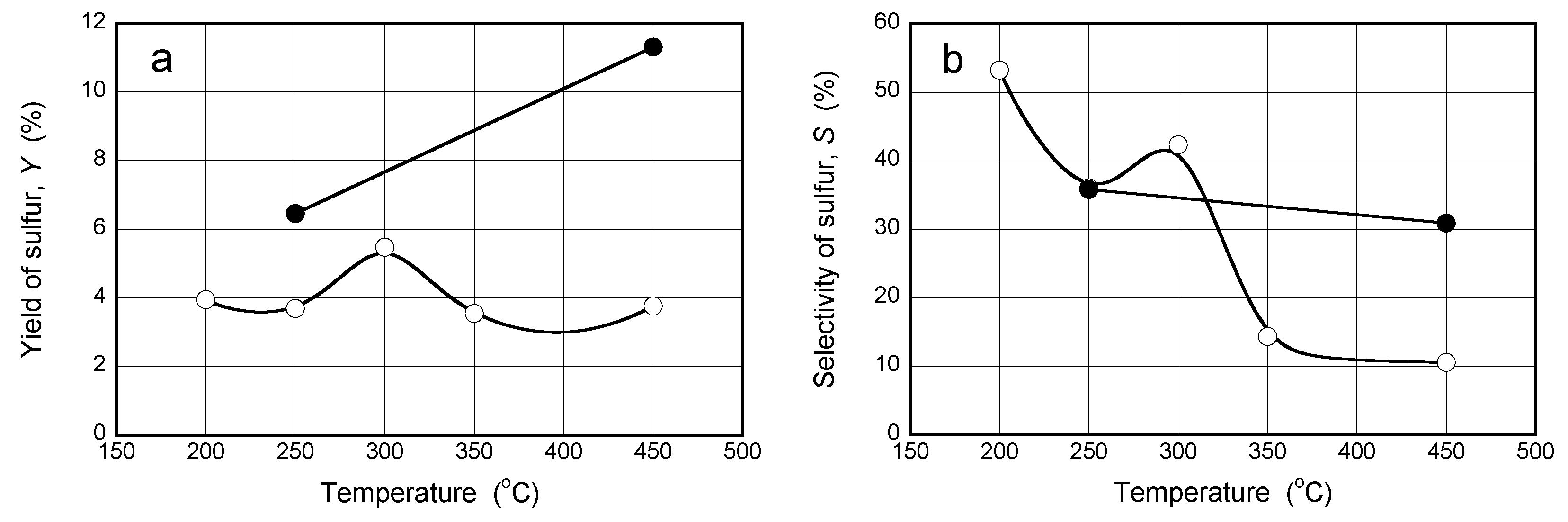
In Figure 4b, the conversion for the base-case conditions for all the limes are presented with the temperature. The long term runs were made to see if a maximum conversion could be achieved in practice if the residence time is very high. TGA results showed that 84% lime conversion is the limit for lime B and C, and 91% for lime A [33]. These values are based on what can be achieved for a reaction with CO${}_2$ according to the TGA experiments. As seen from Figure 4b, only lime C is close to the maximal value, displaying 76% conversion at 450 ${}^{\circ }$C. In the case of short term experiments, increasing the temperature increases the total conversion for all limes. For long term experiments, lime B shows the same conversion with temperature while the other limes still show an increase in conversion. Further, the total conversion is very low in the case of lime A, even for the long term experiments. Such low conversion makes it difficult to draw conclusions about the kinetics of this lime. However, data indicate that the kinetics at 450 ${}^{\circ }$C are superior for lime C, at least in comparison with lime B, since the conversion after the short term experiment is close to that after the long term one.

The sulfur yields with temperatures are presented for base-case conditions in Figure 5a, for lime B and C. The yield after the long term run is much better than the yield after the short term experiment for both the limes. In addition, at 450 ${}^{\circ }$C, the yield shown by lime C is significantly better compared to lime B at the same temperature. Moreover, lime B shows a pronounced drop in yield when going from 350 ${}^{\circ }$C (or 250 in case of the long runs) to 450 ${}^{\circ }$C and this drop is supported by both the short and the long experiments.

The selectivity for sulfur with the temperature is shown in Figure 5b for the same experimental conditions as for Figure 5a. The selectivity for the long runs is also higher than for the short runs for both the limes. In the short experiments, the selectivity for lime C shifts to lower values between 250 ${}^{\circ }$C and 350 ${}^{\circ }$C while in the case of lime B, the selectivity lowers at 450 ${}^{\circ }$C. For lime B, the selectivity (Figure 5b) decreases when going from 350 ${}^{\circ }$C (or 250 in case of long term experiments) to 450 ${}^{\circ }$C, just as the yield also decreases in Figure 5a. Such a drop is shown in both the short and long tests.

The yield and selectivity of sulfur for lime A are shown in Figure 6a and Figure 6b, respectively. The sulfur yield for lime A is between 3% to 6% for all temperatures in the case of short term experiments. At 250 ${}^{\circ }$C, the yield is still low even for the long term run. The yield for the long term experiment with lime A at 450 ${}^{\circ }$C is comparable with that of lime B. On the other hand, the selectivity of lime A is much higher until 300 ${}^{\circ }$C when compared to lime B and C. Above that temperature, the selectivity falls considerably for lime A. The selectivity for lime A at 250 ${}^{\circ }$C is very close for both short term and long term experiments, suggesting no improvement in selectivity with time. However, there is a considerable improvement in selectivity with time at 450 ${}^{\circ }$C.

3.4. The Effect of CO${}_2$ for Lime A

The experiments with lime A were repeated with 10% CO${}_2$ in the inlet stream for 150, 350 and 450 ${}^{\circ }$C, to investigate the effect of the concentration of CO${}_2$ on the performance of the lime for SO${}_2$ capture (see Table 3 for experimental conditions). The experiments with lower CO${}_2$ concentration represent the conditions for air-fired plants as in the case of [20,21,22,29,30,31].

The 60% CO${}_2$ curve in Figure 7a is the same as the one in Figure 4a for lime A. It is here compared with the times for 90% SO${}_2$ breakthrough when the CO${}_2$ is decreased to 10% and further to 0%. The time taken for the breakthrough of 10% SO${}_2$ is higher with lower concentrations of CO${}_2$, but only at 450 ${}^{\circ }$C. At other temperatures, it is relatively unaffected within the measurement error. The time required for 90% of the SO${}_2$ to breakthrough is much higher than in the case of 10% CO${}_2$ as compared to that of 60% when the temperature is 150 or 450 ${}^{\circ }$C. While at 350 ${}^{\circ }$C, there is no difference in breakthrough times. In the case of 0% CO${}_2$ concentration, the 90% SO${}_2$ breakthrough time shows an increase with temperature. As mentioned in Table 3, the experiment at 450 ${}^{\circ }$C with 0% CO${}_2$ was not conducted to let 90% of the SO${}_2$ breakthrough. The time shown in Figure 7a for 0% CO${}_2$ and 450 ${}^{\circ }$C corresponds to that of 84% SO${}_2$ breakthrough.

The conversions of lime A for short term experiments are displayed in Figure 7b, for different CO${}_2$ concentrations in the inlet. The conversion is the highest for lime A, at above 70% at 450 ${}^{\circ }$C, if CO${}_2$ is lowered to 10%. The conversions at other temperatures are close to that of 60% CO${}_2$. The conversion of lime for 0% CO${}_2$ is also close to that of 60% CO${}_2$ at 350 ${}^{\circ }$C. At 450 ${}^{\circ }$C, the conversion is lower when compared to 10% CO${}_2$ case, probably because the experiment was terminated at only 84% SO${}_2$ breakthrough. In Figure 7c, the yield for the different concentrations of CO${}_2$ are compared for lime A. The yield in the case of 10% CO${}_2$ concentration is only slightly higher than that of 60% CO${}_2$ case when the temperature is 150 and 350 ${}^{\circ }$C. However, the yield at 450 ${}^{\circ }$C is many times higher. With 0% CO${}_2$, the sulfur yield is higher at both 350 and 450 ${}^{\circ }$C.

As seen in Figure 7d, the selectivity for 10% CO${}_2$ is higher than for 60%, for all three temperatures. We only have data at three temperatures for 10% CO${}_2$, so we do not know if the performance between 200 and 300 ${}^{\circ }$C could be equally erratic for 10% CO${}_2$ as for 60% CO${}_2$ concentration. As expected, the sulfur selectivity is 100% in the absence of CO${}_2$ at 350 ${}^{\circ }$C. This is also reflected in the conversion of lime (Figure 7b) and the yield of sulfur (Figure 7c); they show the same value of about 25%. As shown in Equation (1), $Y=S·X/100$, when $S=100$%, $Y=X$. At 450 ${}^{\circ }$C however, the selectivity is lower as the experiment was terminated at 84% SO${}_2$ breakthrough. The sulfated lime is thermodynamically more stable and unreactive in air but, the unreacted lime is still "available" for reaction and can be “infected” by CO${}_2$ from the air when sent to analysis. This affects the selectivity and therefore, lower selectivity is observed in Figure 7d. This is shown as a disparity in Figure 7b,c. The conversion of lime is higher than the yield of sulfur in the case of 0% CO${}_2$ at 450 ${}^{\circ }$C.

A summary of the data from Figure 7b–d, in terms of the enhancement, when cutting the CO${}_2$ down to 10%, is shown in Figure 8a. Yet again, a large difference is observed at 450 ${}^{\circ }$C; the conversion of lime is twice as high for the experiments with 10% CO${}_2$ compared to 60% CO${}_2$, whereas the selectivity for SO${}_2$ is thrice as high and the yield is more than six times higher.

3.5. Effect of Water Vapor for Lime A

The experiments at 350 ${}^{\circ }$C and 450 ${}^{\circ }$C were repeated with lime A to investigate what happens when the concentration of water vapor is cut from 25% to 0%, with both 60% and 0% CO${}_2$ (see Table 4 for experimental conditions). As per the thermodynamic analysis, in the absence of H${}_2$O, dehydration of lime is favorable at both the temperatures. However, the TGA in the presence of air (Figure 3a), showed that the kinetics of dehydration onset at 380 ${}^{\circ }$C despite the thermodynamics being favorable at 350 ${}^{\circ }$C. The H${}_2$O concentration in the present experiments were 0% while the TGA was performed in air, i.e., with low but non-zero water vapor content. It is still noteworthy that the kinetics of the dehydration step is low at 350 ${}^{\circ }$C but reaches its maximum at 450 ${}^{\circ }$C as per the TGA.

Figure 8b shows an enhancing effect when cutting water from 25% to 0%, probably due to dehydration as predicted by thermodynamics. It has been established already that dehydration of lime enhances the performance for desulfurization [2]. This enhancement effect is slight at 350 ${}^{\circ }$C and most pronounced at 450 ${}^{\circ }$C with high CO${}_2$ concentration as compared to the case of no CO${}_2$. Figure 3a prompts to higher dehydration rate at 450 ${}^{\circ }$C as compared to 350 ${}^{\circ }$C but, the increase in lime conversion and sulfur yield are not significant, if any, as the temperature increases from 350 ${}^{\circ }$C to 450 ${}^{\circ }$C in the absence of CO${}_2$. In the presence of CO${}_2$, however, not only does the overall conversion of lime increase more than two times, the yield of sulfur increases more than 2.5 times. Such higher effect on sulfur yield compared to the conversion of lime shows that the dehydration not only opens up new unreacted lime surfaces for SO${}_2$ and CO${}_2$ capture, it “prefers” sulfur capture to carbon capture. Notably, the yield at 450 ${}^{\circ }$C without CO${}_2$ are overestimated due to the value in the denominator being error prone. As mentioned earlier, experiment at 450 ${}^{\circ }$C with 0% CO${}_2$ and 25% H${}_2$O was terminated with 84% SO${}_2$ breakthrough. Therefore, the improvement might be slightly lower.

Li et al. have found a similar enhancement in sulfation of lime with a decrease in moisture content from 16% to 8%. They have also observed a simultaneous increase in lime decomposition rates and attributed the increase in sulfation to availability of CaO for reaction. However, they have observed an increase in carbonation in contrast to our results. Furthermore, their temperature range was higher, between 450–570 ${}^{\circ }$C for convective pass application, and their CO${}_2$ concentration was only 14% [30]. In contrast, Stewart et al. tested limestone for sulfation at high temperature (850 ${}^{\circ }$C) and found that increased H${}_2$O improved sulfation and conversion in case of both air-fired as well as oxy-fuel cases [4].

4. Discussion

The yield of sulfur is a key parameter. It is a measure of the absolute amount of sulfur which has reacted with the lime. If the yield increases with time, it means that more species react with the lime. Consequently, if the yield decreases with time, the corresponding species disappears from the lime. This is exactly what can be seen for carbonate under certain conditions. The most obvious case is for lime C at 450 ${}^{\circ }$C when going from short to long term experiments. The conversion of lime increased from 72% to 77% (Figure 4b) i.e., $\Delta X=$ +5% and the yield of sulfur increased from 13% to 25% (Figure 5a) i.e., $\Delta Y_{\left(S{O}_2\right)}$ = +12%. It then follows that the carbon yield decreases from 59% to 52% (calculated based on the description in the methods section), i.e., $\Delta Y_{\left(C{O}_2\right)}=\Delta X-\Delta Y_{\left(S{O}_2\right)}$ = −7%. Hence, the following reaction has been proven under these conditions:

$$\mathrm{CaCO}{}_3+\mathrm{SO}{}_2+1/2{\mathrm{O}}_2\rightleftharpoons \mathrm{CaSO}{}_4+\mathrm{CO}{}_2$$

Li et al. also observed a similar reaction pathway. The amount of CaCO${}_3$ increased and then decreased further with time while sulfur capture increased simultaneously, prompting towards the above reaction pathway [29]. Additionally, this small change in conversation over long exposure times raises an interesting question about the kinetics. Figure 4b indicates that the kinetics for lime C are superior at 450 ${}^{\circ }$C since the conversion for short term exposure is close to that for long term. However, this is only true for the formation of carbonate, as seen from the relatively lower selectivity (Figure 5b) for short term experiments compared to the long term experiments at 450 ${}^{\circ }$C. The time span between short and long term runs is needed to replace some of the carbonate with sulfate and to further capture sulfur, as seen in Figure 5a.

Looking at the overall behavior of lime C with temperature, the 90% SO${}_2$ breakthrough time (Figure 4a) increases between 200 to 250 ${}^{\circ }$C, stays constant at the same value between 250 and 350 ${}^{\circ }$C and further increases when the temperature increases to 450 ${}^{\circ }$C. On the other hand, the sulfur selectivity (Figure 5b) shows a two-step behavior. The selectivity that is constant from 200 to 250 ${}^{\circ }$C steps down when the temperature is increased to 350 ${}^{\circ }$C and stays constant when the temperature is further increased to 450 ${}^{\circ }$C. Combining the 90% breakthrough time with sulfur selectivity allows for the prediction of sulfur yield (Figure 5a) behavior. The conversion for lime C, in Figure 4b, is much higher than the yield values because of the reaction between the lime and CO${}_2$ for the short term tests.

In the case of lime B, the breakthrough times for 90% SO${}_2$ (Figure 4a) decrease with the temperature while the selectivity (Figure 5b) is mostly constant until 350 ${}^{\circ }$C and decreases drastically at 450 ${}^{\circ }$C. The behavior of 90% breakthrough times and selectivity with temperatures together explain the yield (Figure 5a) for lime B. The yield at 450 ${}^{\circ }$C is low owing to both low selectivity as well as low breakthrough times. The increase in conversion (Figure 4b) on the other hand, is due to the carbonation reaction. The long term selectivity for sulfur increases at both 250 and 450 ${}^{\circ }$C, increasing the long term yield and conversion. Selectivity (Figure 5b) and yield (Figure 5a) for sulfur are very low in the case of lime B at 450 ${}^{\circ }$C. In light of the conversion data from Figure 4b, it is clear that lime B “prefers” CO${}_2$ rather than SO${}_2$ at 450 ${}^{\circ }$C, as shown by two independent experiments.

In case of lime A, the breakthrough times for 90% SO${}_2$ increased with the temperature for base-case conditions (Figure 4a). The sulfur selectivity (Figure 6b) for short term experiments displays erratic behavior due to the poor performance of lime A, i.e., since the yield and conversion values are so low, the errors in selectivity calculation are higher. However, it shows a broadly decreasing trend with the temperature for the short term experiments. The combination of breakthrough times and selectivity, together explain the behavior of yield (Figure 6a), which is more or less constant for the short term experiments over the temperature range. The steady increase of conversion with the temperature for the short term experiments, despite the low selectivity, is because of the carbonation reaction. Nevertheless, in the case of the long term experiments, the reaction between CaCO${}_3$ and SO${}_2$ ensures that the selectivity for sulfur is higher at 450 ${}^{\circ }$C. The fact that the conversion (Figure 4b) does not increase for the 12 h experiments shows that the predominant reaction taking place at 450 ${}^{\circ }$C, in the long run, is the conversion of CaCO${}_3$ to CaSO${}_4$, as is evident from an increase in selectivity for sulfur (Figure 6b) in the case of long term exposure. Inexplicably, even though a total conversion of more than 70% was achieved with 10% CO${}_2$ and short experiment time (Figure 7b), such high total conversion was not achieved with 60% CO${}_2$ despite running for 12 h (Figure 4b).

The results show that desulfurization at medium temperature range (250–450 ${}^{\circ }$C) in oxy-fuel combustion should be aiming at moderate SO${}_2$ removal. The results from our work suggest that lime B is suitable for injection in the cooler end of the economizer or warmer end of the duct system while lime C is best suited for injection in the economizer under oxy-fuel conditions. On the other hand, lime A might be better suited for air-fired plants. There is no simple explanation for this behavior based on the properties of the lime types shown in Table 1. In order to meet the emission standard, there is a need for further sulfur capture in a wet FGD system. Furthermore, the conversion of lime, even after 12 h of reaction, never reached 100% conversion and most of the used lime contained carbonate from reaction of the lime and CO${}_2$. The spent sorbent obtained from the medium temperature sulfur capture, therefore, has excellent properties to be re-used in the downstream wet FGD system. The spent sorbent will contain substantial amounts of limestone (calcium carbonate) and lime (calcium hydroxide), the former being the standard reagent in wet FGD and latter being an even superior reagent. The percentage of available reagent contained in the spent sorbent can be estimated as $(100-Y_{\left(S{O}_2\right)})$, and the lime-to-limestone ratio is $(100-Y_{\left(C{O}_2\right)}-Y_{(S{O}_2}))/Y_{\left(C{O}_2\right)}$. Furthermore, the use of the spent sorbent contains the same end product as will be obtained in wet FGD, i.e., calcium sulfate.

5. Conclusions

Medium temperature desulfurization was tested with oxy-fuel conditions using three different limes. The effect of temperature, CO${}_2$ concentration and water vapor were also investigated. It was found that the desulfurization behavior depends strongly on the lime type. In case of lime A, the effect of water vapor and CO${}_2$ were also tested, and sulfur capture was better in the absence of water vapor, particularly at 450 ${}^{\circ }$C with 60% CO${}_2$. Additionally, removing water improved SO${}_2$ capture far better than CO${}_2$ capture at these conditions. With lower CO${}_2$ concentration, there was a marked increase in total conversion along with sulfur yield and selectivity, at least at 450 ${}^{\circ }$C and short term experiments. The total conversion was more than 70% for the short term experiment with 10% CO${}_2$ while a long run with 60% CO${}_2$ resulted in only about 35% conversion of lime. Higher residence times allowed for a different pathway for sulfur capture via reaction of CaCO${}_3$ and SO${}_2$.

Lime A was found to be better suited for air-fired applications, while lime B and C are suitable for oxy-fuel plants. To optimize the sulfur capture over carbon capture, lime B should be injected in the cooler end of the economizer or warmer end of the duct system while lime C can be injected in the economizer. There is no simple explanation to this behavior based on the properties of the lime types investigated. Moreover, medium temperature desulfurization should be used in combination with other desulfurization units. The produce from medium temperature desulfurization can be re-used as SO${}_2$ sorbent in the wet FGD unit.

References

1. Soud, H.N.; Takeshita, M. FGD Handbook, IEACR/65, 2nd ed.; IEA Coal Research: London, UK, 1994; pp. 467–506. [Google Scholar]
2. Miller, B.G. Formation and Control of Sulfur Oxides. Clean Coal Eng. Technol. 2011, 1, 467–506. [Google Scholar]
3. Wang, C.B.; Zhang, Y.; Jia, L.F.; Tan, Y.W. Effect of water vapor on the pore structure and sulphation of CaO. Fuel 2014, 130, 60–65. [Google Scholar] [CrossRef]
4. Stewart, M.C.; Symonds, R.T.; Manovic, V.; Macchi, A.; Anthony, E.J. Effects of steam on the sulfation of limestone and NOX formation in an air- and oxy-fired pilot-scale circulating fluidized bed combustor. Fuel 2012, 92, 107–115. [Google Scholar] [CrossRef]
5. Wang, C.B.; Jia, L.F.; Tan, Y.W.; Anthony, E.J. The effect of water on the sulphation of limestone. Fuel 2010, 89, 2628–2632. [Google Scholar] [CrossRef]
6. Allen, D.; Hayhurst, A.N. Reaction between gaseous sulfur dioxide and solid calcium oxide mechanism and kinetics. J. Chem. Soc. Faraday Trans. 1996, 92, 1227–1238. [Google Scholar] [CrossRef]
7. Anthony, E.J.; Granatstein, D.L. Sulfation phenomena in fluidized bed combustion systems. Prog. Energy Combust. Sci. 2001, 27, 215–236. [Google Scholar] [CrossRef]
8. Low, M.J.D.; Goodsel, A.J.; Takezawa, N. Reactions of Gaseous Pollutants with Solids. 1. Infrared Study of Sorption of SO2 on CaO. Environ. Sci. Technol. 1971, 5, 1191–1195. [Google Scholar] [CrossRef]
9. Hartman, M.; Coughlin, R.W. Reaction of Sulfur-Dioxide with Limestone and Influence of Pore Structure. Ind. Eng. Chem. Process. Des. Dev. 1974, 13, 248–253. [Google Scholar] [CrossRef]
10. Suyadal, Y.; Erol, M.; Oguz, H. Deactivation model for dry desulphurization of simulated flue gas with calcined limestone in a fluidized-bed reactor. Fuel 2005, 84, 1705–1712. [Google Scholar] [CrossRef]
11. Munoz Guillena, M.J.; Linares Solano, A.; de Lecea, C.S.M. High temperature SO2 retention by CaO. Appl. Surf. Sci. 1996, 99, 111–117. [Google Scholar] [CrossRef]
12. Liu, C.F.; Shih, S.M.; Lin, R.B. Kinetics of the reaction of Ca(OH)2/fly ash sorbent with SO2 at low temperatures. Chem. Eng. Sci. 2002, 57, 93–104. [Google Scholar] [CrossRef]
13. Liu, C.F.; Shih, S.M.; Huang, T.B. Effect of SO2 on the Reaction of Calcium Hydroxide with CO2 at Low Temperatures. Ind. Eng. Chem. Res. 2010, 4, 9052–9057. [Google Scholar] [CrossRef]
14. Karatepe, N.; Ersoy-Mericboyu, A.; Yavuz, R.; Kucukbayrak, S. Kinetic model for desulphurization at low temperatures using hydrated sorbent. Thermochim. Acta 1999, 335, 127–134. [Google Scholar] [CrossRef]
15. Irabien, A.; Cortabitarte, F.; Viguri, J.; Ortiz, M.I. Kinetic-Model for Desulfurization at Low-Temperatures Using Calcium Hydroxide. Chem. Eng. Sci. 1990, 45, 3427–3433. [Google Scholar] [CrossRef]
16. Izquierdo, J.F.; Fite, C.; Cunill, F.; Iborra, M.; Tejero, J. Kinetic study of the reaction between sulfur dioxide and calcium hydroxide at low temperature in a fixed-bed reactor. J. Hazard Mater. 2000, 76, 113–123. [Google Scholar] [CrossRef]
17. Klingspor, J.; Strömberg, A.-M.; Karlsson, H.T.; Bjerle, I. Similarities between lime and limestone in wet-dry scrubbing. Chem. Eng. Process. 1984, 18, 239–247. [Google Scholar] [CrossRef]
18. Lee, K.T.; Koon, O.W. Modified shrinking unreacted-core model for the reaction between sulfur dioxide and coal fly ash/CaO/CaSO4 sorbent. Chem. Eng. J. 2009, 146, 57–62. [Google Scholar] [CrossRef]
19. Lee, K.T.; Mohamed, A.R.; Bhatia, S.; Chu, K.H. Removal of sulfur dioxide by fly ash/CaO/CaSO4 sorbents. Chem. Eng. J. 2005, 114, 171–177. [Google Scholar] [CrossRef]
20. Fernández, I.; Garea, A.; Irabien, A. SO2 reaction with Ca(OH)2 at medium temperatures (300–425 C): Kinetic behaviour. Chem. Eng. Sci. 1998, 53, 1869–1881. [Google Scholar] [CrossRef]
21. Fernández, I.; Garea, A.; Irabien, A. Flue-gas desulfurization at medium temperatures. Kinetic model validation from thermogravimetric data. Fuel 1998, 77, 749–755. [Google Scholar] [CrossRef]
22. Hünlich, T.; Jeschar, R.; Scholz, R. Sorption Kinetics of SO2 from Combustion Waste Gases at Low-Temperatures. Zement-Kalk-Gips 1991, 4, 228–237. [Google Scholar]
23. Svoboda, K.; Lin, W.; Hannes, J.; Korbee, R.; van den Bleek, C.M. Low-temperature flue gas desulfurization by alumina-CaO regenerable sorbents. Fuel 1994, 73, 114–1150. [Google Scholar] [CrossRef]
24. García-Martínez, J.; Bueno-López, A.; García-García, A.; Linares-Solano, A. SO2 retention at low temperatures by Ca(OH)2-derived CaO: A model for CaO regeneration. Fuel 2002, 81, 305–313. [Google Scholar] [CrossRef]
25. Muñoz-Guillena, M.J.; Linares-Solano, A.; de Lecea, C.S.M. A study of CaO-SO2 interaction. Appl. Surf. Sci. 1994, 81, 409–415. [Google Scholar] [CrossRef]
26. Muñoz-Guillena, M.J.; Linares-Solano, A.; de Lecea, C.S.M. A study of CaO-SO2 interaction in the presence of O2. Appl. Surf. Sci. 1994, 81, 417–425. [Google Scholar] [CrossRef]
27. Muñoz-Guillena, M.J.; Linares-Solano, A.; de Lecea, C.S.M. A new parameter to characterize limestones as SO2 sorbents. Appl. Surf. Sci. 1995, 89, 197–203. [Google Scholar] [CrossRef]
28. Miller, B.G. Anatomy of a Coal-Fired Power Plant; Butterworth-Heinemann: Oxford, UK, 2011. [Google Scholar]
29. Li, G.G.; Keener, T.C.; Wang, J. A Two-Stage Reactor for Studying Sorbent Reactivities in Flue Gas Desulfurization Systems Utilizing a Fabric Filter Collector. Environ. Technol. 1998, 19, 475–482. [Google Scholar] [CrossRef]
30. Li, G.; Keener, T.; Stein, A.; Khang, S. CO2 reaction with Ca(OH)2 during SO2 removal with convective pass sorbent injection and high temperature filtration. Environ. Eng. Policy 2000, 2, 47–56. [Google Scholar]
31. Li, G.G.; Keener, T.C.; Stein, A.W. Continuous Sorbent Reactions in a High-Temperature Fabric Filter Following Convective Pass Ca(OH)2 Injection for SO2 Removal. J. Air Waste Waste Manag. Assoc. 1999, 49, 1292–1303. [Google Scholar] [CrossRef]
32. Chen, J.; Yao, H.; Zhang, L. A study on the calcination and sulphation behaviour of limestone during oxy-fuel combustion. Fuel 2012, 102, 386–395. [Google Scholar] [CrossRef]
33. Wang, W.; Sanku, M.; Karlsson, H.; Hulteberg, C.; Karlsson, H.T.; Balfe, M. Medium Temperature Desulfurization for Oxyfuel and Regenerative Calcium Cycle. Energy Procedia 2017, 114, 271–284. [Google Scholar] [CrossRef]
34. Perez-Ramirez, J.; Berger, R.J.; Mul, G.; Kapteijn, F.; Moulijn, J.A. The six-flow reactor technology—A review on fast catalyst screening and kinetic studies. Catal Today 2000, 60, 93–109. [Google Scholar] [CrossRef]
35. Himmelblau, D.M.; Riggs, J.B. Basic Principles and Calculations in Chemical Engineering, 5th ed.; Prentice-Hall: Upper Saddle River, NJ, USA, 1989. [Google Scholar]
Figure 1. Schematic of air-fired power plants (drawn based on information in [2]). 1-Furnace (1100 to 1250 C), 2-Superheater/Reheater (600 to 1100 C), 3-Economizer (300 to 600 C), 4-Duct system (50 to 250 C), 5-Baghouse, 6-Air heater, a-Coal, b-Hot gases from combustion, c-Air. The temperatures in each region are indicative and prone to vary from plant to plant.
Energies 12 02645 g001
Figure 2. Schematic of experimental setup used. 1-Mass flow controller, 2-Syringe, 3-Reactor, 4-Gas analyzer, 5-Fume hood, 6-Feedback temperature control, a-SO 2 /N 2 , b-N 2 , c-O 2 , d-CO 2 , e-Water, (–) Process line, (...) Electrical line, (=) Electrical tracing.
Energies 12 02645 g002
Figure 3. (a) (▪) TGA in % mass, (•) dTG in % mass/min and, (▴) DSC in mW, of lime A in air. (...) Marking onset of change in DSC. The results for the other limes were similar, and TGA in air for all limes can be found in [33]. (b) TGA of lime samples in 100% CO 2 [33]. Re-printed from [33], which is licensed under a Creative Commons license (https://creativecommons.org/licenses/by-nc-nd/4.0/) (c) dTG of lime samples in 100% CO 2 (d) DSC of lime samples in 100% CO 2 In Figure 3b–d, the legend is as follows: (◯) Lime A, (▵) Lime B, (□) Lime C.
Energies 12 02645 g003
Figure 4. (a) Time for 10% and 90% SO 2 breakthrough for short term experiments of all lime types; (◯) Lime A, 10% (▵) Lime B, 10% (□) Lime C, 10% (•) Lime A, 90% (▴) Lime B, 90% (▪) Lime C, 90% (b) Conversion for both short and long term experiments for all lime types. (◯) Lime A, short term (▵) Lime B, short term (□) Lime C, short term (•) Lime A, long term (▴) Lime B, long term (▪) Lime C, long term. The inlet conditions were 2000 ppm SO 2 , 25% H 2 O, 2.5% O 2 and 60% CO 2 .
Energies 12 02645 g004
Figure 5. (a) Yield of sulfur with temperatures and (b) Selectivity of sulfur with temperatures under the inlet conditions of 2 000 ppm SO 2 , 25% H 2 O, 2.5% O 2 and 60% CO 2 . In both figures, the legend is as follows: (▵) Lime B, short term (□) Lime C, short term (▴) Lime B, long term (▪) Lime C, long term.
Energies 12 02645 g005
Figure 6. (a) Yield of sulfur with temperatures and (b) Selectivity of sulfur with temperatures under the inlet conditions of 2000 ppm SO 2 , 25% H 2 O, 2.5% O 2 and 60% CO 2 . In both figures, the legend is as follows: (◯) Lime A, short term (•) Lime A, long term.
Energies 12 02645 g006
Figure 7. (a) Time for 10% and 90% SO 2 breakthrough with lime A for different concentrations of CO 2 . (◯) 0% CO 2 , 10% SO 2 breakthrough (▵) 10% CO 2 , 10% SO 2 breakthrough (□) 60% CO 2 , 10% SO 2 breakthrough (•) 0% CO 2 , 90% SO 2 breakthrough (▴) 10% CO 2 , 90% SO 2 breakthrough (▪) 60% CO 2 , 90% SO 2 breakthrough (b) Conversion of lime (c) Yield of sulfur (d) Selectivity for sulfur for different concentrations of CO 2 with lime A. In Figure 7b–d, the legend is as follows: (◯) 0% CO 2 , (□) 10% CO 2 , (□) 60% CO 2 In all the figures, (X) marks the experiment where only 84% breakthrough of SO 2 was observed before termination. The other concentrations are as per base-case experiments.
Energies 12 02645 g007
Figure 8. (a) Ratios of X (conversion of lime), S (Selectivity for sulfur) and Y (yield of sulfur capture) when dividing the values for the parameters at 10% CO 2 by the corresponding values at 60% CO 2 ; (blue): X @10% CO 2 /@60% CO 2 ; (grey): S @10% CO 2 /@60% CO 2 ; (red): Y @10% CO 2 /@60% CO 2 ; (b) Ratios of X (conversion of lime) and Y (yield of sulfur capture) when dividing the values of the parameters at 0% H 2 O by the corresponding values at 25% H 2 O for different CO 2 concentrations; (black): X @0% H 2 O/@25% H 2 O for 0% CO 2 ; (blue): X @0% H 2 O/@25% H 2 O for 60% CO 2 ; (grey): Y @0% H 2 O/@25% H 2 O for 60% CO 2 ; (red): Y @0% H 2 O/@25% H 2 O for 0% CO 2 . The experiments were conducted using lime A. The concentrations that are not specified in the figures are as per base-case experiments.
Energies 12 02645 g008