Abstract
Combustion condition monitoring is a fundamental and critical issue that needs to be addressed in the wide-load operation of coal-fired boilers. In this paper, an unsupervised classification framework based on the convolutional auto-encoder (CAE), the principal component analysis (PCA), and the hidden Markov model (HMM) is proposed to monitor the combustion condition with the uniformly spaced flame images, which are collected from the furnace combustion monitoring system. First, CAE is adopted to extract the features from the flame images, which obtain the sparse representations in the images. Then, PCA is applied to project the feature vectors into the orthogonal space for robustness and computation efficiency. Finally, a HMM is built to calculate the corresponding optimal states by learning the temporal behaviors in the compressed representations. A coal combustion adjustment experiment was conducted in a 660 MW opposed-firing boiler, and the sequential 14,400 flame images with three different combustion states were obtained to evaluate the effectiveness of the proposed approach. We tested six different compression dimensions of the latent variable z in the CAE model and ensured that the appropriate compress parameter was 1024. The proposed framework is compared with five other methods: the CAE + Gaussian mixture model (GMM), CAE + Kmean, the CAE + fuzzy c-mean method, CAE + HMM, and the traditional handcraft feature extraction method (TH) + HMM. The results show that the proposed framework has the highest classification accuracy (95.25% for the training samples and 97.36% for the testing samples) and has the best performance in recognizing the semi-stable state (85.67% for the training samples and 77.60% for the testing samples), indicating that the proposed framework is capable of identifying the combustion condition, changing when the combustion deteriorates as the coal feed rate falls.
1. Introduction
Fossil power plants in China are facing more peak-shaving requests for the growth of renewable energies. Reducing the minimum unit technique output is one of the goals of flexible transformation, which means the boilers in power plants should be operated below the designed minimum output. When the boiler runs in a low load, the changeable quality of coal used in practice makes the combustion unstable, which directly affects the safety and economics of the boiler operation. Hence, the identification of combustion condition has received extensive attention by researchers. Flame visualization and characterization techniques are some of the research tools for understanding the combustion process. Current research mainly includes feature-based machine learning, statistical-based process monitoring, and deep learning methods.
The main steps of feature-based machine learning methods are feature extraction and state classification. However, whether or not the extracted characteristic parameters could represent the combustion condition is dependent on the image processing technology, such as the segmentation algorithm. Machine learning mainly includes artificial neural networks, linear classifiers, and clustering analysis, and tuning the parameters usually takes lot of time. Back propagation (BP) neural network (NN) [1], wavelet NN [2], and a method combined with Kohonen’s self-organizing NN and BP [3] were proposed to predict combustion status based on digital images. For improving the convergence speed and recognition accuracy, Han et al. [4] proposed an interactive flame image recognition method in which manual evaluation was introduced to the NN. Considering the uncertainty in flame detection, Li et al. [5] proposed a two-stage fusion structure, combining BP and the Dempster–Shafer (D–S) evidence theory. To analyze the dynamic characters in the flame images, Liu et al. [6] selected the relative changes of the ignition position as the inputs of the fuzzy neural network, Zhang et al. [7] applied the fuzzy theory to fuse the fire detection value and flame characteristics, and Xu et al. [8] proposed an online fuzzy clustering algorithm to monitor the in-furnace combustion states automatically. In terms of the linear classifiers, the support vector machine (SVM) [9] and the robust support vector regression machine [10] are also proposed for their anti-outlier performance. Wu et al. [11] introduced the Krawtchouk moment and Wang et al. [12] used Fisher Discriminant Analysis to extract the features, then combined wavelet SVM and k-nearest neighbor (KNN) for combustion state classification. For the sintering process of a rotary kiln, Li et al. [13] applied the ensemble learner models with the probabilistic neural network (PNN), the NN, the SVM, and extreme learning machine (ELM) classifiers for combustion state recognition and Chen et al. [14] used SVM and ELM to recognize the temperature condition of a rotary kiln.
On combustion process monitoring, Bai et al. [15] proposed a principal component analysis (PCA) to extract the characteristics of flame images. Considering the stochastic behavior of time series in the combustion process, Chen et al. [16] proposed a framework based on multiway principal component analysis (MPCA) and the hidden Markov model (HMM) to establish the probability monitoring chart of oil flame images under a normal combustion state for the combustion transition state sequence tracking. Bai et al. [17] proposed a multi-condition combustion process monitoring method based on a principal component analysis and random weight network (PCA-RWN).
In recent years, deep learning has received unprecedented attention and development. Its greatest advantage is that it can learn the representative characteristics in data automatically and avoid misleading from hand-crafted features [18]. It is widely applied in research fields related to feature extraction: Zhou et al. [19] combined independent subspace analysis (ISA) with a convolutional network to extract the local morphology of the burning image for the rotary kiln sintering process layer by layer and built the word package model to learn its global feature. Yuting et al. [20] used a deep belief network (DBN) to obtain features in the image of the furnace flame. In combustion state recognition, Wang et al. [21] proposed a deep learning method based on convolutional neural network (CNN) and deep neural network (DNN) to monitor combustion states and predict the heat release rate.
The studies above were mainly based on supervised learning, that is, the models learn and extract the corresponding features, directly and intentionally, through the information feedback from the labeled images. These labels are often given by researchers through specific experimental conditions or expertise. It’s a time-consuming and laborious task to label the image manually. If mistakes are made in the process of labeling, they would affect the performance of the models. The Kohonen network, proposed by Wei [2], and a fuzzy immune network algorithm, proposed by Guo et al. [22], were the attempts to realize the unsupervised learning in the flame monitoring process. However, since the features are extracted by hand-craft, it is hard to determine whether the selected features could improve the optimal recognition performance for combustion state classification.
In this paper, we propose an unsupervised classification framework based on the convolutional auto-encoder (CAE), principal component analysis (PCA), and the hidden Markov model (HMM) for pulverized coal combustion status recognition with the uniformly spaced flame images. The effective characteristics of the flame images are retrieved with the CAE and then further compressed with PCA to obtain a set of orthogonal data. The hidden Markov model is built on the orthogonal data and applied to new flame images for combustion status recognition. In the framework, the CAE is applied to extract features from the flame images directly, which simplifies the whole feature extraction process compared with the hand-craft method; PCA is introduced to disentangle the latent space, in which the data exists as relevant relationships in a good representation subspace, to make the different features independent of each other; HMM is applied to capture the dynamic temporal behaviors, which are effective for combustion condition recognition. In this paper, six different compression dimensions of the latent variable z in the CAE model are compared to select the appropriate compress parameter. The framework is then tested with the flame images from a 660 MW thermal power plant and compared with other methods, including the CAE + Gaussian mixture model (GMM), CAE + Kmean, the CAE + fuzzy c-mean method, CAE + HMM, and the traditional handcraft feature extraction method (TH) + HMM, to verify the effectiveness of the proposed framework.
2. Methodology
2.1. Convolutional Auto-Encoder
CAEs differ from conventional AEs as their weights are shared among all locations in the input and are preserved in spatial locality. The details of CAEs can be found in [23,24]. For a mono-channel input , the latent representation of the -th feature map is given by [23],
where the bias and weight are broadcasted to the whole map, is a nonlinear transformation (we use the rectified linear units (ReLU) [25] function here), and “” denotes the 2-dimensional convolution. The reconstruction process can be calculated as [23],
where H identifies the group of latent feature maps, identifies the flip operation over both dimensions of the weights, and is the bias for each input channel. The cost function to minimize the reconstruction error between the input and output is the binary cross entropy, which can be written as [26],
where is the number of samples.
2.1.1. Max-Pooling
For hierarchical networks, in general, and CNNs, in particular, a max-pooling layer is often introduced to obtain translation-invariant representations by taking the maximum value over the non-overlapping sub-region [23]. Figure 1b shows the down-sampling process of the input matrix , which is divided into several sub-regions. If the sub-regions do not overlap and the size of a sub-region is , the -th sub-region can be expressed as [27]
where is the -th blocks in the matrix .
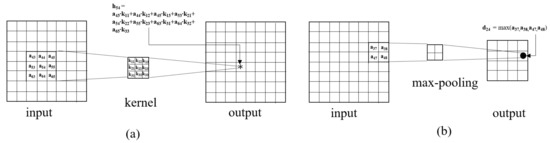
Figure 1.
The schematics of (a) the convolutional process and (b) the down-sampling process.
The max-pooling for is defined as [27]
The non-overlap max-pooling for matrix with the sub-region’s size is defined as [27]
2.1.2. Activation
The activation layer mainly performs nonlinear transformation on the input data, so that the network can fit nonlinear projection. The commonly used activation functions are sigmoid [26] and rectified linear units (ReLU). Sigmoid has the exponential function shape to imitate the biological neuron, which is located in the final layer to produce a categorical probability distribution, and is defined as [26].
The ReLU function is a piecewise function, which can change all the negative values to 0, and has better performance than the sigmoid function in terms of calculation speed. The function can be written as [25].
2.2. Principal Component Analysis (PCA)
As described in the previous sections, we can get the feature matrix from the output of the encoder. If the -th feature vector is , then the feature matrix can be written as
where is the number of features and is the number of samples. The auto-encoder compresses the original data into a more compact representation, which contains the most important features by reconstructing the input. PCA projects the input into an orthogonal space, ensuring that the obtained lower-dimension vector components are independent of each other. The goal of PCA [28] is to find the orthonormal matrix in , where the rows of are the principal components of . The singular value decomposition of the correlation matrix of , i.e., is given by [17]
where represents a unitary matrix and is the diagonal matrix of the eigenvalues. If is the number of the principal components, then the loading matrix can be marked as . The score matrix is calculated as [17]
where is a matrix transformed from , by reducing the n-dimensional feature vectors to r-dimensional vectors.
2.3. The Hidden Markov Model (HMM)
The HMM is a double stochastic process, in which the transition probability between each state and the observations of each state are uncertain [16,17,18,29]. The state that exists in the model can only be perceived through the vector and cannot be observed directly. We used the notation as the parameter set of the HMM model. represents the state transition probability distribution, which is the state transition probability among hidden states, and is the number of states. We denote the individual states as and the state at time as . The transition distribution is defined as [29]
if is the initial state distribution, where
The observation distribution is generalized by a Gaussian density [29],
where is the set of the observation vectors collected for modeling, is the mixture coefficient for the -th mixture in state and it should be summed up to one for each state, is the Gaussian density with mean vector , and the covariance matrix is the th mixture component in state .
Given some observation sequences as training data, we can use an iterative procedure, such as the Baum–Welch procedure, to estimate the model parameters, and the details are explained in [29]. The goal is to adjust the parameters of the model to maximize . If is the single best state sequence from a given , then the quantity can be defined as [29]
where is the highest probability along the single path when the state ends in at time . By induction we have [29]
Finally, we can get the formula of , i.e., the combustion state to its corresponding observation sets [29]
2.4. CAE and PCA-HMM-Based Combustion Classificaion
Applying image processing technology can retrieve rich and reliable information from the flame images. It has been widely studied and applied in various fields. In the sintering process of the rotary kiln, a flame image-based burning state recognition system is used to ensure sintered clinkers are qualified [19]. In the process of basic oxygen furnace blowing, it is used to make accurate and real-time judgment of the furnace endpoint [30]. In the aero-engine, it is proposed to determine the combustor ignition/flameout status and retrieve its corresponding features directly [31]. In this paper, we propose a deep learning method with pulverized flame images to recognize the burner state, which has a great reference value when applying it to the image-based combustion status recognition in other fields.
Figure 2a shows the schematic diagram of the proposed methods and the distribution map of swirl burners in the opposed-firing boiler. The A, B, C, D, E, F, and G in Figure 2a represent the seven layers of burners, which were distributed on the front and back wall of the furnace. The C, D, E, and F layer burners were on the front wall and the A, B, and G layer burners were on the back wall. Every layer burner was equipped with a medium-speed coal mill, and the pulverized coal pipelines of each coal mill were connected to the corresponding layer burners. Each mill and its corresponding layer burners could be shut down according to the boiler load changing. The flame image monitoring system, including a probe and a protective sleeve for each burner, was mounted on the F layer burners, as shown in Figure 2b. The cooling air pipelines were installed to cool the probe, which was extended into the furnace, ensuring that the probe’s temperature did not exceed 70. The images of coal combustion in the furnace were captured by the image probe as a video format, transferred through the composite video cables, and stored in the hard disk recorder in the electronics room. Firstly, we transformed the flame videos into the red, green, and blue (RGB) images with the size of 960 × 576 × 3 under 25 frames per sec frame rate, using video processing technology, and calculated the average of the 25 images per sec to eliminate the influence of the flicker. Secondly, the images were resized to the size of , as the inputs of the CAE model. The CAE model learns to encode the input images in compact representations and then reconstructs the input images from these representations. By training the CAE model, the representations can hold key information about the input images. Subsequently, PCA was applied to project the representations as feature vectors into the orthogonal space, ensuring that the feature vector components were independent of each other. Finally, the HMM model was built to generate the corresponding optimal state sequence from the feature variables, which can be applied for online combustion condition monitoring. The framework was built with the following steps:
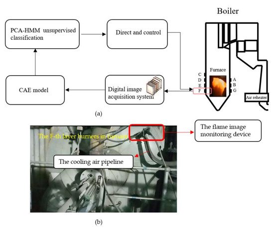
Figure 2.
(a) The schematic diagram of the proposed convolutional auto-encoder (CAE) and principal component analysis and hidden Markov model (PCA-HMM) framework for combustion classification and the position of seven layer burners in the boilers with the C, D, E, and F layers of burners on the front wall and the A, B, and G layers on the back wall; (b) The site installation of the flame image monitoring device.
- (1)
- A CAE model was constructed, in which the latent variables were considered as the features of the flame images , where is the number of the nodes in the encoding network’s output and is the numbers of the flame images.
- (2)
- The loading matrix was calculated to transform the n-dimensional latent variables into the r-dimensional data using PCA, and was taken as the observation vectors in the HMM model.
- (3)
- A set of was collected as the training data, and the parameters of the HMM model were estimated using Baum–Welch algorithm.
- (4)
- The output of the HMM model was calculated as , where is the highest probability along the path when the state ends in at time , and is the corresponding hidden state of .
3. Result and Discussion
3.1. Data Preparation
To evaluate the performance of the proposed framework, a coal combustion adjustment experiment was conducted in a opposed-firing boiler. The lines in Figure 3a,b are the actual total load in the training samples and the testing samples during the period of 11:00–17:00. The lines in Figure 3c,d are the coal rate of the F mill. The coal rate was adjusted to make the combustion state of the F layer burners gradually change between stable and unstable. According to the combustion theory [32], the concentration of the pulverized coal is the most important factor directly influencing the pulverized coal ignition and combustion in the airflow. For example, if the concentration of the pulverized coal is low and the amount of heat released is small, then a continuous flame cannot be formed. The large external heat dissipation makes the temperature level decrease, leading to unstable combustion. In the coal combustion adjustment experiment, as shown in Figure 3c, the coal rate was relatively steady at during 11:00–12:00, which means the combustion state was stable; then the coal rate of the F mill began to decrease around 14:35, until it was at 14:45; finally, the coal rate began to increase at 15:02 until the combustion stable state was reached. The combustion was under poor stability when the coal rate was around . We sampled the sequential 14,400 flame images as training sets and the 3600 images for testing sets. In particular, due to the lack of unstable and semi-stable samples, we selected the flame images between the period of 14:00–15:00, both as training and testing data. To differentiate testing data from the training data, we took the average images of 2 s during 13:00–15:00 as the testing data. The selected time periods are shown in Table 1. Figure 4 shows three typical images representing different combustion statuses, in which the combustion status of the flame from left to right are stable, semi-stable, and unstable, respectively.
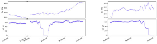
Figure 3.
The related variables in the boiler operation process: (a) The actual total load in the training data; (b) the actual total load in the testing data; (c) the coal rate of the F mill in the training data; (d) the coal rate of the F mill in testing data.

Table 1.
The selected time periods in the coal combustion experiment.
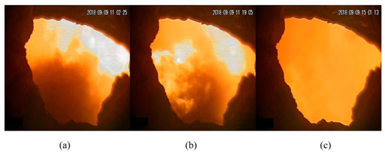
Figure 4.
Typical flame images under different combustion statuses: (a) Stable; (b) semi-stable; (c) unstable.
3.2. Simulation
3.2.1. Convolutional Auto-Encoder
We adjusted the image size from to as the input of the CAE network. The procedure was performed in the computer equipped with an Intel i7-CPU and a Nvidia GeForce GTX 1060 GPU (MI, Beijing, China). Figure 5 shows the architecture of the CAE network and the process of the encoding and decoding. The encoder consists of three convolutional layers, three max-pooling layers, and two fully connected layers. All convolutional layers use kernels, followed by ReLU activation functions and max-pooling layers, with with the stride of 2. We flattened the output of the last max-pooling layer into a one-dimensional vector and compressed it into the smaller dimensions with two full connection layers. The decoding structure was completely symmetrical with the encoding structure, which contained fully connected layers, convolutional layers, and un-pooling layers. The sigmoid activation function was applied in the last layer of the decoder to produce the output . Here, we chose the cross-entropy as a loss function to measure the deviation between the reconstructions and the original images . Table 2 shows the structure and parameters of the CAE network, where represents the kernel size, is the step size, is the number of the kernels, and is the fill parameter.
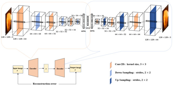
Figure 5.
The architecture of the CAE network.
Table 2.
Structure and parameters of the CAE network.
3.1.2. Determinate in the Compression Dimensions of Latent Variable
In this section, we explore the compression limit of the latent representation z to ensure that it has small dimensions but still contains enough useful information to reconstruct the original images closely. According to the CAE’s architecture, we tested six different dimensions in the calculation. Figure 6 shows the comparison between the original images and the model’s outputs. When the dimensions of the latent variables are 4096, 2048, and 1024, as shown in Figure 6b–d, the decoded images are diversified, similar to the original images, as shown in Figure 6a, and there is little difference among the three rows of flame images. The decoded images of the CAEs with latent dimensions as 512 and 256, respectively, as shown in Figure 6e,f are blurred and hardly satisfactory in some parts of the images. When the latent dimension is set to , the latent representation contains too little information to reconstruct the input, and there is almost no difference among the right three decoded images in Figure 6g.
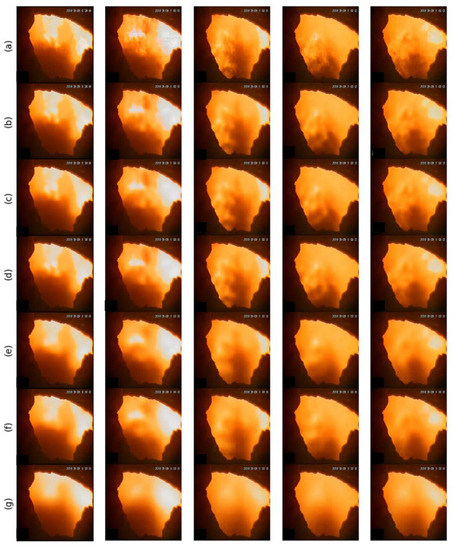
Figure 6.
The original flame images and reconstructions of the CAE networks: (a) Original images; (b) the decoded images of the CAE networks with different latent representation , as 4096, (c) 2048, (d) 1024, (e) 512, (f) 256, and (g) 2.
The object of training the CAE network is to use as few dimensions as possible to reconstruct the input, and the reconstructed images should be as similar as the original images. Figure 7 shows the mean square error (MSE) among different dimensions, and Table 3 shows the corresponding values. The MSE changes slightly when the dimensions are greater than 1000. We choose 1024 as the appropriate dimensions for the latent representation .
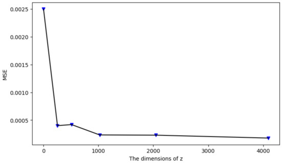
Figure 7.
The mean square error (MSE) of the CAE networks with different latent representations.
Table 3.
The MSE of the CAE networks with different latent representations.
3.1.3. Using PCA and HMM
In the previous section, we selected 1024 as the appropriate dimensions parameter for and took the latent representation as the feature vector of the flame image. PCA is applied here to reduce the dimensions of the feature vector, to improve the computational efficiency, and to avoid overfitting, due to the redundancy in the images. We used PCA to descend the high-dimensional data into a 90-dimensional vector with a contribution rate of . As the observation sets, the compressed vectors were used to train the HMM, assuming that the number of the hidden states is . By the iterative procedure, we obtained the model parameters and got the optimal state sequence corresponding to the observation sets.
Besides the proposed framework, we implemented another five methods for comparison: CAE + GMM, CAE + kmeans, CAE + fuzzy c-means, CAE + HMM, and TH + HMM:
- Since the HMM is proposed in this paper, we chose three different unsupervised clustering algorithms for comparison: the Gaussian Mixture model [33], k-means [34], and Fuzzy c-means [35]. For the four methods, including CAE, we took the latent variables obtained by CAE as the inputs of the clustering model and then set the labels by these methods respectively.
- TH adopts the traditional feature extraction procedure to get the feature vector of a flame image. We preprocessed the flame images before the feature extraction: (1) The median filter was applied for image denoising; (2) the QSTU algorithm [36] was applied for image segmentation. A total of 18 features were extracted, including the RGB image’s first-order and second-order moment, the gray level co-occurrence matrix (angular second moment, entropy, inverse differential moment, and correlation) [17], the fractal dimension [36], the flame’s area, and the first-order and second-order moment of the images’ HSI (hue,saturation,intensity) space [37]. The extracted vectors were taken as the observation sets, to get the optimal hidden state distribution using HMM.
3.1.4. Experimental Results and Analysis
In order to evaluate the performance of the proposed framework effectively, we got the real labels of the flame images, according to three intervals of the coal rate. Table 4 shows the specific ranges of coal rate. In addition, the combustion stability classification should not only reflect the combustion condition changes, but should also reflect the flicker frequency during the combustion process. We selected the following criteria to evaluate the performance: The flame image was considered as the stable state when the combustion status was changing between unstable and stable within 10 s; if the unstable (non-fire) state lasted for at least 10 s, the flame image was considered as the unstable state.
Table 4.
The specific ranges of coal rate and combustion status.
Figure 8a shows the comparison of different methods on the training data. Each point represents the combustion state corresponding to the flame image per second. Combining with the specific ranges of the coal rate (Table 4), the red dots represent the actual states: Category 0, 1, and 2, which represent unstable, semi-stable, and stable, respectively. From the distribution of the red dots, we can see that the unstable state remains at 14:45–15:02 when the coal rate was around 0 t/h; the semi-stable state remains at 14:35–14:45 and 15:02–15:09 when the coal rate was increasing or decreasing between 27 t/h and 53 t/h during those periods. As shown in Figure 8a, these methods, except the fuzzy c-means method (the pink dots), have higher accuracy in recognizing the unstable states; the Gaussian mixture model (the violet dots) and k-means algorithm (the yellow dots) have poor performance in identifying the semi-stable state. The methods that obtain HMMs, such as CAE + HMM (the brown dots), TH + HMM (the green dots), and CAE + PCA − HMM (the blue dots), have relatively steady performance in recognizing the combustion states. In particular, the proposed framework has the most ideal output. The results show that the HMM has an advantage in processing time series, in which the HMM can capture the temporal behaviors in the characteristic parameters and detect the change of combustion status more accurately. The conventional k-means is especially not suitable for this classification task, since the data has temporal behavior. The classification accuracy could be enhanced using the semi-supervised learning algorithms, such as discriminative k-means method [38], which needs further research.
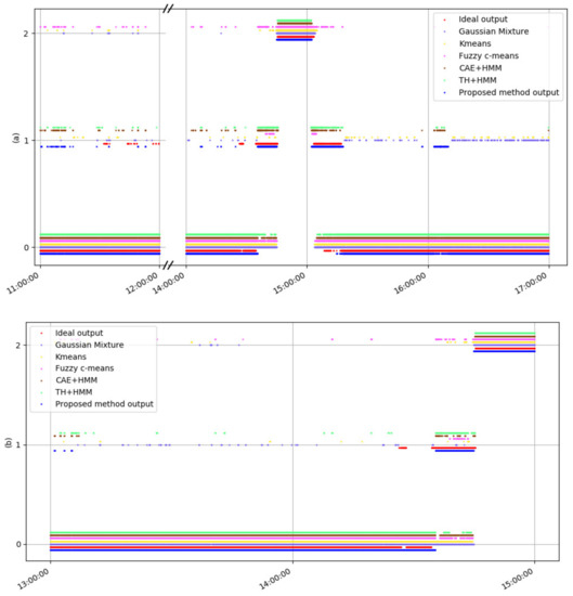
Figure 8.
(a) The hidden states distribution of the training data via different methods; (b) the hidden states distribution of the testing data via different methods. For better observation, the results of some methods are shifted up (or down) a little, based around the actual values.
Figure 8b shows the results of different methods on the testing data. In the figure, each point represents the combustion state corresponding to the flame image every 2 s. As in Figure 8a, the red dots represent the actual states over the combustion process. The Gaussian mixture model, k-means, and fuzzy c-means methods could not identify the semi-stable state well. All the methods except the proposed framework have a higher error rate in considering the semi-stable state as the stable state.
Under the aforementioned criteria, the performance of the proposed framework, CAE + GMM, CAE + Kmeans, CAE + fuzzy c-mean, CAE + HMM, and TH + HMM were evaluated with the same sets of flame images, and their confusion matrices are shown in Figure 9. It can be seen from Figure 9a–e that these methods have higher accuracy for category and , while they have bad performance in category . The classification accuracy of the GMM, k-means, and fuzzy c-means in the semi-stable state are 0.0026, 0.0123, and 0.059, respectively, which mean that these clustering methods can’t capture the sequential correlation in the flame characteristic. The lower accuracy of the CAE + HMM in this case implies that the observations set contains many correlated variables, which affects the performance of combustion state classification. TH was only about half accurate in category (0.4948). Since the feature extraction process was performed manually, we cannot guarantee that the feature vectors acquired are comprehensive and repetitive.
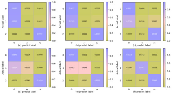
Figure 9.
The confusion matrices of different methods on the training data: (a) Convolutional auto-encoder and Gaussian mixture model (CAE + GMM); (b) CAE + k-means; (c) CAE + fuzzy−c-means; (d) CAE + HMM; (e) traditional handcraft and hidden Markov model (TH + HMM); (f) CAE + PCA + HMM.
Table 5 shows the classification accuracy of different methods on training data. It is worth noting that the total accuracy of the TH + HMM method is close to the proposed framework, indicating that the extracted features, such as the brightness and texture of the image, can reflect the change of combustion state effectively. It can be explained that CAE can extract useful features in the flame images effectively.
Table 5.
Accuracy of the training data via different methods.
The confusion matrices of these methods in testing data are shown in Figure 10. Table 6 shows the specification of the classification accuracy in testing data. The results show that all the methods have high accuracy in identifying the unstable and stable states; however, they have worse performance in the semi-stable states, among which the k-mean has the lowest accuracy (0.0301) and the proposed method has the highest accuracy (0.7760). The results show that the proposed framework has excellent performance in recognizing the semi-stable state, which is of great significance to guide the coal combustion adjustment.
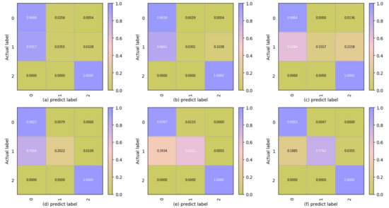
Figure 10.
The confusion matrices of different methods on the testing data: (a) CAE + GMM; (b) CAE + k-means; (c) CAE + fuzzy−c-means; (d) CAE + HMM; (e) TH + HMM; (f) CAE + PCA + HMM.
Table 6.
Accuracy of the testing data via different methods.
4. Conclusions
In this study, an unsupervised framework combined CAE, PCA, and HMM is proposed to classify the coal combustion status. First, we tested the influence of latent representation variables () in CAE with different dimensions on coal combustion adjustment experiment results, and was selected as the suitable parameter, which made the CAE contain the useful and sufficient features to closely reconstruct the input data. PCA was then applied to compress and de-nose the latent representation and to ensure that the vector components in the latent representation were independent and the computing was efficient. Finally, we adopted the HMM to learn and capture the sequence correlation in the combustion process.
In order to verify the effectiveness of the model, the coal rate was selected as the classification criteria of the combustion state, according to the combustion theory. The classification accuracy of the proposed framework on the training data and testing data were 95.25% and 97.36%, respectively. In particular, the proposed framework had better performance in recognising the semi-stable state (85.67% for the training samples and 77.60% for the testing samples), which is important for adjusting the combustion state in advance to avoid unstable combustion. It can therefore be concluded that the proposed framework not only simplifies the feature extraction process compared with manual image processing, but also provides an effective means for classifying the flame combustion status in an unsupervised way.
Author Contributions
Methodology, T.Q.; project administration (guided and coordinated combustion adjustment experiment), G.Z.; supervision, L.W. and K.G.; writing—Original draft, M.L.; writing—Review and editing, T.Q. and M.L.
Funding
This research was funded by the National Key R&D Program of China, grant number (NO. 2017YFB0902100).
Conflicts of Interest
The authors declare no conflict of interest.
Abbreviations
| CAE | convolutional autoencoder |
| CNN | convolution neural network |
| GMM | Gaussian mixture model |
| HMM | hidden Markov model |
| PCA | principal component analysis |
| TH | traditional handcraft feature extraction method |
| transition distribution | |
| mixture coefficient | |
| optimal state in time | |
| z | latent variable (latent representation) |
| mean vector | |
| initial state distribution | |
| parameters of the HMM model | |
| highest probability along the single path when the state ends in at time | |
| number of states | |
| Gaussian density | |
| observation vectors in time | |
| the loading matrix | |
| individual states | |
| unitary matrix | |
| covariance matrix | |
| diagonal matrix of the eigenvalues |
References
- Wang, F.; Ma, Z.Y.; Yan, J.H.; Wang, X.J.; Zhao, J.; Ni, M.; Cen, K.F. Diagnosis of Furnace Flame by Computer Image Processing and Neural Network Technology. Therm. Power Gener. 2003, 32, 24–28. (In Chinese) [Google Scholar]
- Chen, C.Y.; Yan, J.H.; Shang, M.; Ma, Z.Y.; Wang, X.; Cen, K.F. Combustion Diagnosis Based on Flame Image in Furnace. Power Eng. 2003, 32, 24–28. (In Chinese) [Google Scholar]
- Xu, Z.W. Recogniton and Diagnosis of Boiler Flame Based on Wavelet Neural Network. Chin. J. Sci. Instrum. 2004, 25, 376–379. (In Chinese) [Google Scholar]
- Han, P.; Zhang, X.; Wang, B.; Pan, W.H. Interactive Method of Furnace Flame Image Recognition Based on Neural Network. Proc. CSEE 2008, 28, 22–26. (In Chinese) [Google Scholar]
- Li, Z.X. Research on Furnace Flame Detection Based on MSIF; North China Electric Power University: Heibei, China, 2009. (In Chinese) [Google Scholar]
- Liu, H. Judging boiler combustion stability based on flame image and fuzzy neural network. Chin. J. Sci. Instrum. 2008, 29, 1280–1284. (In Chinese) [Google Scholar]
- Zhang, X.; Ding, Y.J.; Zheng, K.J.; Wu, Z.S. Combustion state evaluation of swirl burner based on multi-source information fusion. Proc. CSEE 2010, 30, 23–28. (In Chinese) [Google Scholar]
- Xu, B.C.; Zhang, D.Y.; Chen, L. Study on combustion stability based on flame images. Comput. Eng. Appl. 2012, 48, 168–172. (In Chinese) [Google Scholar]
- Liu, D.G.; Lv, L.X.; Liu, C.L. Flame Furnace in Thermal Power Plant Condition Monitoring Using SVM. In Proceedings of the 2009 Second International Conference on Intelligent Computation Technology and Automation, Changsha, China, 10–11 October 2009. [Google Scholar]
- Chen, X.F.; Wang, S.T; Cui, Y.J.; Ma, Y.P.; Chou, X.Q. Fuzzy Clustering Based Robust SVR and Flame Image Processing. J. Image Graph. 2009, 14, 463–470. (In Chinese) [Google Scholar]
- Wu, Y.Q.; Zhu, L.; Zhou, H.C. State recognition of flame images based on Krawtchouk moment and support vector machine. Proc. CSEE 2014, 34, 734–740. (In Chinese) [Google Scholar]
- Wang, Z.C.; Liu, M.; Dong, M.Y.; Wu, L. Riemannian Alternative Matrix Completion for Image-based Flame Recognition. IEEE Trans. Circuits Syst. Video Technol. 2016, 27, 2490–2503. [Google Scholar] [CrossRef]
- Li, W.; Wang, D.; Chai, T. Flame Image-Based Burning State Recognition for Sintering Process of Rotary Kiln Using Heterogeneous Features and Fuzzy Integral. IEEE Trans. Ind. Inform. 2012, 88, 780–790. [Google Scholar] [CrossRef]
- Chen, H.; Zhang, X.G.; Hong, P.Y.; Yin, X. Recognition of the Temperature Condition of a Rotary Kiln Using Dynamic Features of a Series of Blurry Flame Images. IEEE Trans. Ind. Inform. 2015, 12, 148–175. [Google Scholar] [CrossRef]
- Bai, W.D.; Yan, J.H.; Chi, Y.; Ma, Z.Y.; Zhang, Q.Y.; Lin, B.; Ni, M.J.; Cen, K.F. Research on Flame Monitoring Based on Image Processing Technology and PCA method. Power Eng. 2004, 24, 87–90. (In Chinese) [Google Scholar]
- Chen, J.; Hsu, T.Y.; Chen, C.C.; Cheng, Y.C. Monitoring combustion systems using HMM probabilistic reasoning in dynamic flame images. Appl. Energy 2010, 87, 2169–2179. [Google Scholar] [CrossRef]
- Bai, X.J.; Lu, G.; Hossain, M.M.; Szuhánszki, J.; Daood, S.S.; Nimmo, W.; Yan, Y.; Pourkashanian, M. Multi-mode combustion process monitoring on a pulverised fuel combustion test facility based on flame imaging and random weight network techniques. Fuel 2017, 202, 656–664. [Google Scholar] [CrossRef]
- Wang, S.H.; Xiang, J.W.; Zhong, Y.T.; Zhou, Y.Q. Convolutional neural network-based hidden Markov models for rolling element bearing fault identification. Knowl.-Based Syst. 2018, 144, 65–76. [Google Scholar] [CrossRef]
- Zhou, X.J.; Cai, Y.Q.; Xia, K.J.; Feng, Y. Burning state recognition for rotary kiln sintering process based on burning salient zone image feature learning and classifiers fusion. Control Decis. 2017, 32, 187–192. (In Chinese) [Google Scholar]
- Lyu, Y.T.; Chen, J.H.; Song, Z.H. Image-based process monitoring using deep learning framework. Chemom. Intell. Lab. Syst. 2019. [Google Scholar] [CrossRef]
- Wang, Z.Y.; Song, C.F.; Chen, T. Deep learning based monitoring of furnace combustion state and measurement of heat release rate. Energy 2017, 131, 106–112. [Google Scholar] [CrossRef]
- Guo, J.M.; Liu, S.; Jiang, F. The Application of Fuzzy Immune Network Algorithm to Flame Monitoring. Proc. CSEE 2007, 27, 1–5. (In Chinese) [Google Scholar]
- Masci, J.; Meier, U.; Ciresan, D.; Schmidhuber, J. Stacked Convolutional Auto-Encoders for Hierarchical Feature Extraction. In Proceedings of the Artificial Neural Networks and Machine Learning–ICANN 2011–21st International Conference on Artificial Neural Networks, Espoo, Finland, 14–17 June 2011; Part I. Springer: Berlin/Heidelberg, Germany, 2011. [Google Scholar]
- Gao, Z.S.; Shen, C.; Xie, C.Z. Stacked convolutional auto-encoders for single space target image blind deconvolution. Neurocomputing 2018, 313, 295–305. [Google Scholar] [CrossRef]
- Karimpouli, S.; Tahmasebi, P. Segmentation of digital rock images using deep convolutional autoencoder networks. Comput. Geosci. 2019, 142–150. [Google Scholar] [CrossRef]
- Fang, Z.Q.; Jia, T.; Chen, Q.S.; Xu, M.; Yuan, X.; Wu, C.D. Laser stripe image denoising using convolutional autoencoder. Results Phys. 2018, 11, 96–104. [Google Scholar] [CrossRef]
- Li, Y.J. Deep Learning: Mastering Convolutional Neural Networks from Beginner; Machine Press: Beijing, China, 2018; Volume 424, pp. 33–35. [Google Scholar]
- Shlens, J. A Tutorial on Principal Component Analysis. Int. J. Remote Sens. 2014, 51, 1–12. [Google Scholar]
- Rabiner, L.R. A Tutorial on Hidden Markov Models and Selected Applications in Speech Recognition. Proc. IEEE 1989, 77, 257–268. [Google Scholar] [CrossRef]
- Jiang, F.; Liu, H.; Wang, B.; Sun, X.F. Basic Oxygen Furnace Blowing Endpoint Judgment Method Based on Flame Image Convolution Neural Network. Comput. Eng. 2016, 42, 277–282. [Google Scholar]
- Chen, M.M.; Yuan, T.; Jiang, R.W.; Zhang, X. Application of flame images for combustor ignition/flameout experimentation. Gas Turbine Exp. Res. 2018, 31, 35–37. (In Chinese) [Google Scholar]
- Yan, S.L.; Wang, D.S.; Li, Y.H.; Zhu, W.P. Analysis of the Influential Factors to Boiler Combustion Stability. Power Syst. Eng. 2005, 21, 29–30. (In Chinese) [Google Scholar]
- Reynolds, D. Gaussian Mixture Models. In Encyclopedia of Biometrics; Li, S.Z., Jain, A., Eds.; Springer US: Boston, MA, USA, 2009. [Google Scholar]
- Sculley, D. Web-scale k-means clustering. In Proceedings of the 19th International Conference on World Wide Web, Raleigh, NC, USA, 26 April 2010. [Google Scholar]
- Winkler, R.; Klawonn, F.; Kruse, R. Fuzzy C-Means in High Dimensional Spaces; IGI Global: Hershey, PA, USA, 2011. [Google Scholar]
- Bai, X.J.; Lu, G.; Yan, Y. Fractal Characteristics of Thin Thermal Mixing Layers in Coal-Fired Flame. J. Combust. Sci. Technol. 2017, 23, 225–230. (In Chinese) [Google Scholar]
- Sun, D.; Lu, G.; Zhou, H. Quantitative Assessment of Flame Stability Through Image Processing and Spectral Analysis. IEEE Trans. Instrum. Meas. 2015, 64, 3323–3333. [Google Scholar] [CrossRef]
- Arandjelović, O. Discriminative k-means clustering. In Proceedings of the International Joint Conference on Neural Networks, Dallas, TX, USA, 4–9 August 2013. [Google Scholar]


© 2019 by the authors. Licensee MDPI, Basel, Switzerland. This article is an open access article distributed under the terms and conditions of the Creative Commons Attribution (CC BY) license (http://creativecommons.org/licenses/by/4.0/).