Cogging Torque Reduction in Brushless Motors by a Nonlinear Control Technique

Abstract

This work addresses the problem of mitigating the effects of the cogging torque in permanent magnet synchronous motors, particularly brushless motors, which is a main issue in precision electric drive applications. In this work, a method for mitigating the effects of the cogging torque is proposed, based on the use of a nonlinear automatic control technique known as feedback linearization that is ideal for underactuated dynamic systems. The aim of this work is to present an alternative to classic solutions based on the physical modification of the electrical machine to try to suppress the natural interaction between the permanent magnets and the teeth of the stator slots. Such modifications of electric machines are often expensive because they require customized procedures, while the proposed method does not require any modification of the electric drive. With respect to other algorithmic-based solutions for cogging torque reduction, the proposed control technique is scalable to different motor parameters, deterministic, and robust, and hence easy to use and verify for safety-critical applications. As an application case example, the work reports the reduction of the oscillations for the angular position control of a permanent magnet synchronous motor vs. classic PI (proportional-integrative) cascaded control. Moreover, the proposed algorithm is suitable to be implemented in low-cost embedded control units.

1. Introduction

The phenomenon of cogging torque is an intrinsic characteristic of permanent magnet synchronous motors (PMSMs), in both interior (IPM) and surface-mounted (SPM) electric machine types. This phenomenon is due to the magnetic interaction between the teeth of the stator slots and the permanent magnets arranged on the rotor surface in the SPM case, or internally embedded in the rotor iron in the IPM case [1].

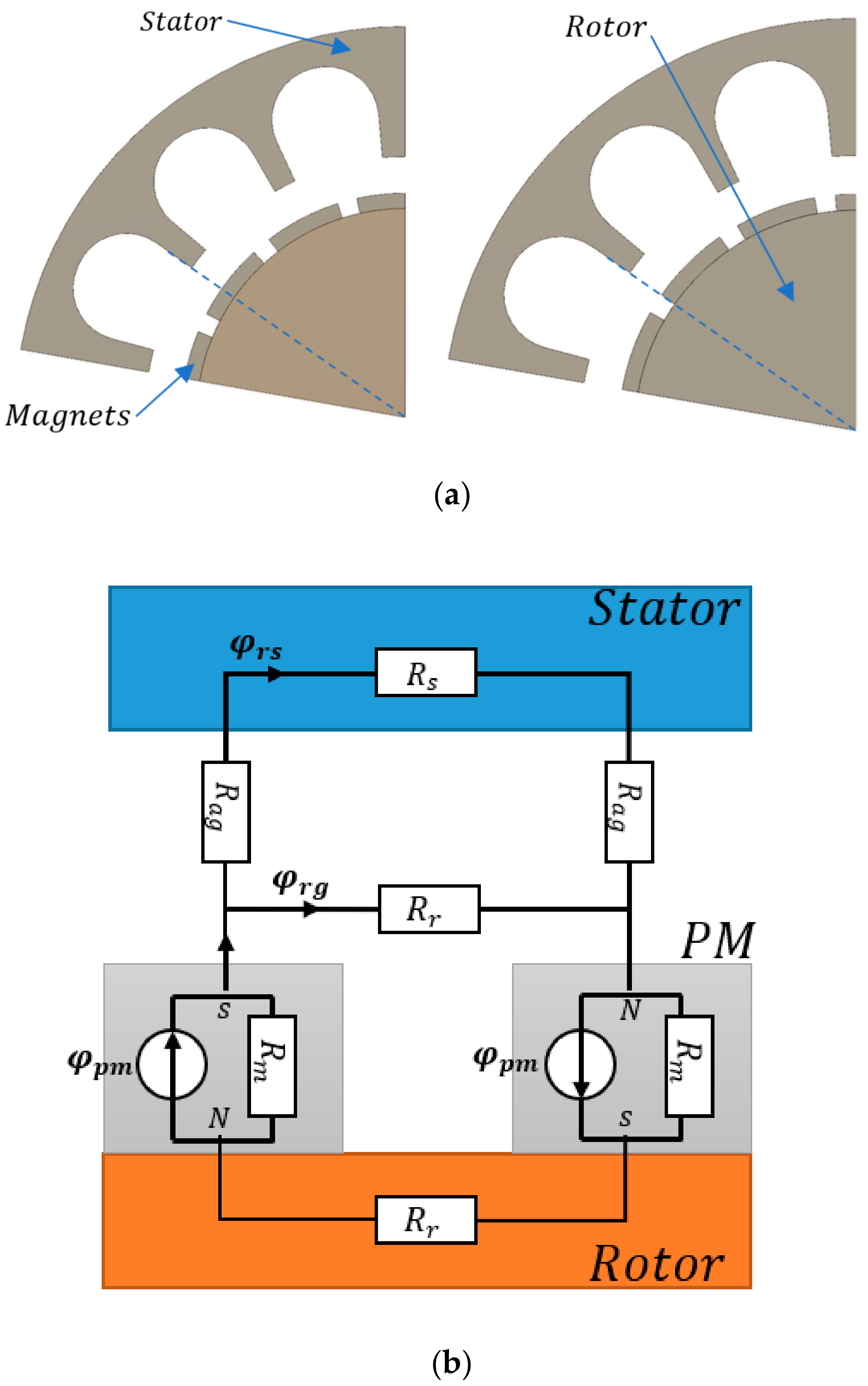
This is because the nonuniformity of the air gap is characterized by an equivalent magnetic circuit, which describes the magnetic interaction between rotor and stator. The equivalent magnetic circuit depends on the mutual position between the teeth of the stator cavities and the permanent magnets. This implies that the reluctance of the magnetic circuit is a function of the rotor angle. Figure 1 shows the physical origins of the cogging couple generating the cogging torque.

In Figure 1, the physical quantity ${\phi }_{pm}$ represents the magnetic flux generated by the permanent magnets, while ${\phi }_{rs}$ and ${\phi }_{rg}$ are the portions closed in the iron of the stator and in the air gap, respectively, and $R_m, R_r, R_s, and R_{ag}$ represent the reluctances of the permanent magnets, rotor, stator, and air gap, respectively.

Figure 1a shows that during the rotation of the rotor, the stator slot will alternately see a polar compartment (the space between two magnets) and a section of a magnet. This confirms that the magnetic circuit changes according to the angular position. Figure 1b represents the path of the magnetic flux in the ideal case of a uniform stator surface.

This phenomenon is due exclusively to the dependence of the magnetic circuit on the angular position and on the magnetic and geometric characteristics of the motor itself. Indeed, it is possible to appreciate the cogging torque even by simply rotating the motor axis manually without electrically feeding it. Starting from an angular position of the rotor, after a rotation of ${\vartheta }_{cog}=2\pi /mcm\left(p,N_c\right)$, where p is the number of pole pairs and $N_c$ is the number of caves, the same situation is encountered. Indeed, along the air gap, the same configuration in terms of interaction between teeth and magnets can be encountered several times. Consequently, the cogging couple is interpretable as a noise disturbance, with an angular frequency dependent on the number of slots and number of magnets and therefore polar pairs. The intensity of the cogging noise disturbance is a function of the geometry of the magnets and the teeth of the slots and of the magnetic characteristics of the materials involved. This disturbance is measurable by means of a test bench where, usually, a brushless motor is mechanically connected to a DC motor (not affected by the cogging effect) and passively rotated. In the mechanical connection of the two rotation axes, a torque meter is incorporated; then, from it, is possible to obtain the torque exerted in the absence of power supply. This torque is therefore equivalent to the torque for cogging effect.

In this work, a method for reducing the cogging torque is proposed, based on the use of a nonlinear automatic control technique. This technique, known as feedback linearization, is ideal for underactuated dynamic systems. State-of-the-art solutions are often based on the physical modification of the electrical machine to try to suppress the natural interaction between the permanent magnets and the teeth of the stator slots. However, such modifications are expensive because they require customized procedures, whereas the proposed method does not require any modification of the electric drive.

This paper is organized as follows. Section 2 reviews the state of the art of cogging reduction techniques that have been recently proposed in the literature and introduces the core idea of the solution proposed. In Section 3, an analytical description of the phenomenon to derive a model useful for the design of an automatic controller is carried out, as well as a model of a brushless motor including the cogging term. Section 4 presents a feedback linearization control to reduce cogging torque in brushless motors. Section 5 presents implementation results and a robustness analysis of the proposed control vs. motor parameter changes. Section 6 presents an analysis of the algorithmic complexity and the suitability for integration in a low-cost embedded system. Conclusions are drawn in Section 7.

2. Review of State of the Art for Cogging Torque Reduction

In the literature, torque ripple due to the cogging couple in PMSMs is reduced, but not eliminated, by an appropriate magnetic and layout winding design, as proposed in [2,3]. The other typical approach is the reduction of the intensity of the magnetic interaction between the stator and the rotor by properly designing the machine according to different criteria and verified with finite element method (FEM) analysis tools, as discussed in [4,5]. The problem with the above approaches is that the modifications to the electrical motor are expensive because are customized, and furthermore, they do not guarantee a complete suppression of the torque ripple caused by the cogging phenomenon. Hence, reduction techniques aiming at modeling and/or estimating the cogging phenomenon and then compensating or reducing it by proper control algorithms are more suited to achieve low-cost and scalable solutions.

The control of the machine stator currents could be used to compensate the torque harmonics that cannot be easily eliminated during the design stage. For instance, a conventional field-oriented control (FOC) scheme is proposed in [6] for torque ripple mitigation. However, because of the relatively high-frequency components present in the torque ripple, high bandwidth currents could be required. In [6,7], this is achieved using dead-beat controllers. Nevertheless, in these studies, the torque ripple is compensated by adding harmonic components in the q-axis stator current reference, and by regulating the d-axis current to zero. Consequently, with $i_d=0$, maximum torque per ampere (MTPA) cannot be achieved [8,9] and the machine is no longer operating at the optimal torque.

In [8], a valid cogging reduction solution has been proposed through the application of the model predictive control (MPC) technique, which is based on solving optimal problems in an iterative manner, which in addition to being computationally heavy, is linked to the knowledge of the model. In recent papers, the use of resonant controllers has been also proposed for the control of PMSMs, such as in [10,11,12].

Resonant controllers are based on the internal model principle and they can be used to regulate with zero steady-state error signals of sinusoidal nature. For this purpose, one resonant notch is required to regulate a single-frequency component of the harmonic torque. Therefore, to eliminate most of the harmonic distortion, multiresonant controllers are required, and the design and digital implementation of such a controller is complex [13]. Moreover, if the control system is implemented in the stationary frame, a tuning mechanism is required to modify the resonant frequencies in real time when variations in the PMSM rotational speed are produced [12].

Recently, the use of finite-control set model predictive control (FCS-MPC) has been proposed for applications involving electrical drives and power converters [14]. With this methodology, a discrete model of the plant and power converter is required to predict the behaviour of the system for a particular switching state of the converter. To track references, a cost function that considers the tracking error at each sampling instant is used. The optimal switching action, which minimizes the cost function, is applied to the converter. As discussed in the literature, FCS-MPC has several advantages. For instance, it is relatively simple to include nonlinearities, constraints, and variables of different nature (electrical or mechanical) in the cost function. The application of FCS-MPC to the control of PMSMs has been discussed in the literature by using predictive current control [15,16]. Additionally, in [17,18], FCS-MPC is suggested as an alternative to a direct regulation of the machine torque. The method is called model predictive direct torque control (MP-DTC), which uses an external speed loop based on a PI controller. However, in previous papers, control methods to reduce the torque ripple produced by flux linkage harmonic distortion are not addressed; neither is mitigation of the cogging torque discussed.

In [19], a torque predictive control to mitigate the high-frequency torque due to switching effects is presented. However, this paper does not address mitigation of the low-frequency torque pulsations produced by the machine.

Control of the PMSM rotational speed based on FCS-MPC is presented in [20,21]. With this approach, the nested control loops typically used in drives are replaced by a predictive control system. The results discussed in [20,21] show that a high dynamic response can be achieved with this methodology. However, to compensate the load torque, an observer has to be implemented, and this may limit the performance of the control system to compensate relatively high-frequency torque components, particularly when the machine is operating at high rotational speed. Moreover, high-bandwidth observers are sensitive to measurement noise, parameter uncertainty, quantization error of the feedback signal, etc. A Lyapunov observer-based control technique is implemented in [22]. With respect to the other approaches based on a control algorithm, the nonlinear control proposed by us allows for an offline and deterministic projection of the control laws. This approach facilitates the integration of a cogging torque model without the need for designing a complex observer to estimate cogging-related signals.

In this work, in the following Sections, a nonlinear control approach is presented as an alternative to all the previous methods. First of all, with respect to [2,3,4,5], the proposed approach has the advantage of keeping the same mechanical structure of the electric motor without adding the payload of customized structures.

The feedback linearization allows to replace the nonlinear dynamic with a linearized one through a systematic change of variables. Furthermore, the proposed control technique is formally more robust than the above-discussed algorithmic techniques for cogging torque mitigation, due to the largest region of asymptotic stability. The proposed algorithm is suitable to be implemented on low-cost embedded controllers; for example, the Arduino-Uno platform using an ATMEGA328 microcontroller.

3. Cogging Torque and Motor Modelling

3.1. Cogging Torque Formulation

In this work, the objective is not to present a method for describing the cogging torque. The starting point is the formulation in closed form, reported in [1], that exploits the Fourier harmonic analysis against results obtained with FEM analysis. In particular, reference was made to the following expression:

$$T_{cog} \cong {\displaystyle \sum }_{k=1}^m{T}_k\sin \left(kZ{\vartheta }_m+ {\alpha }_k\right)$$

(1)

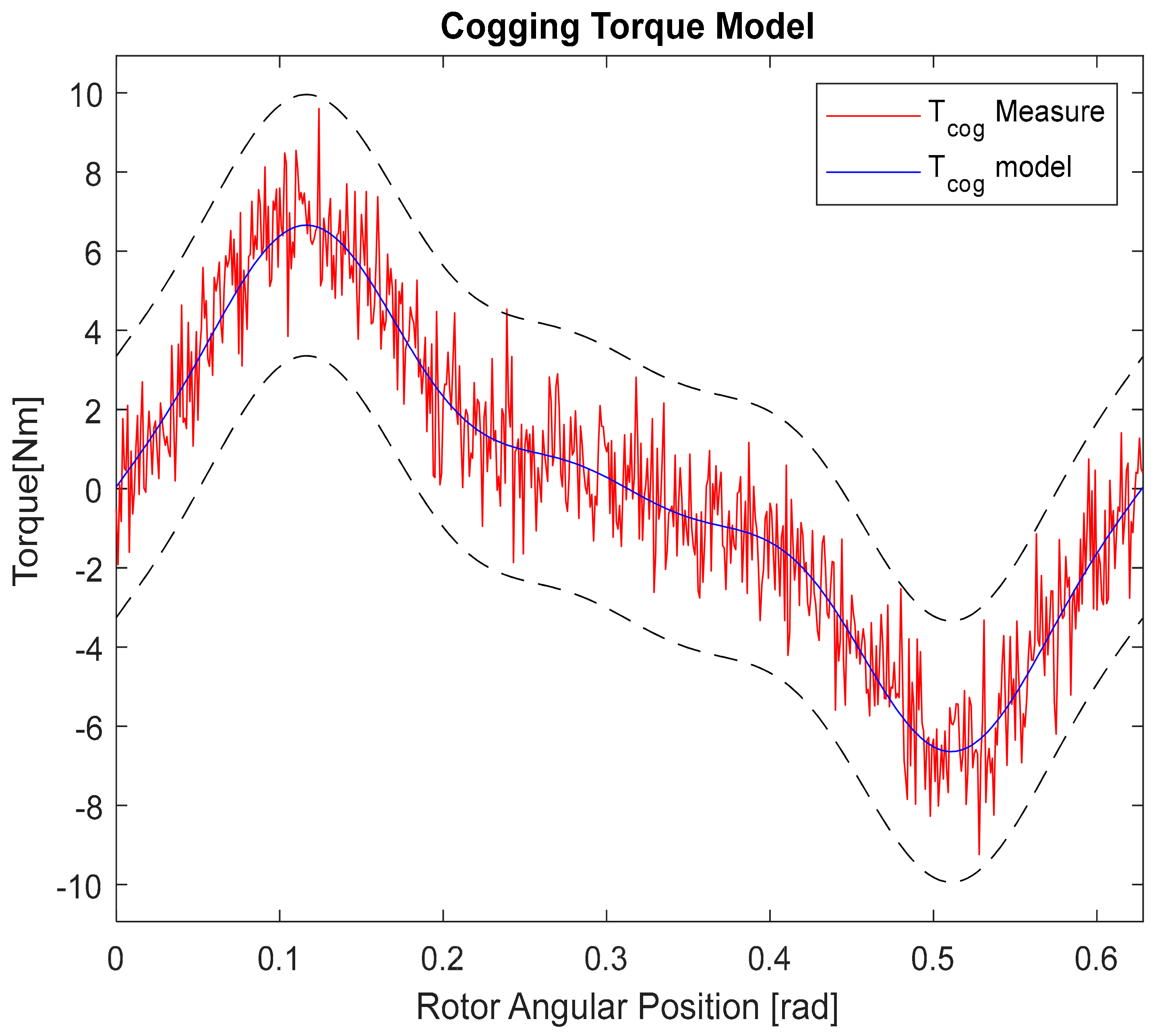
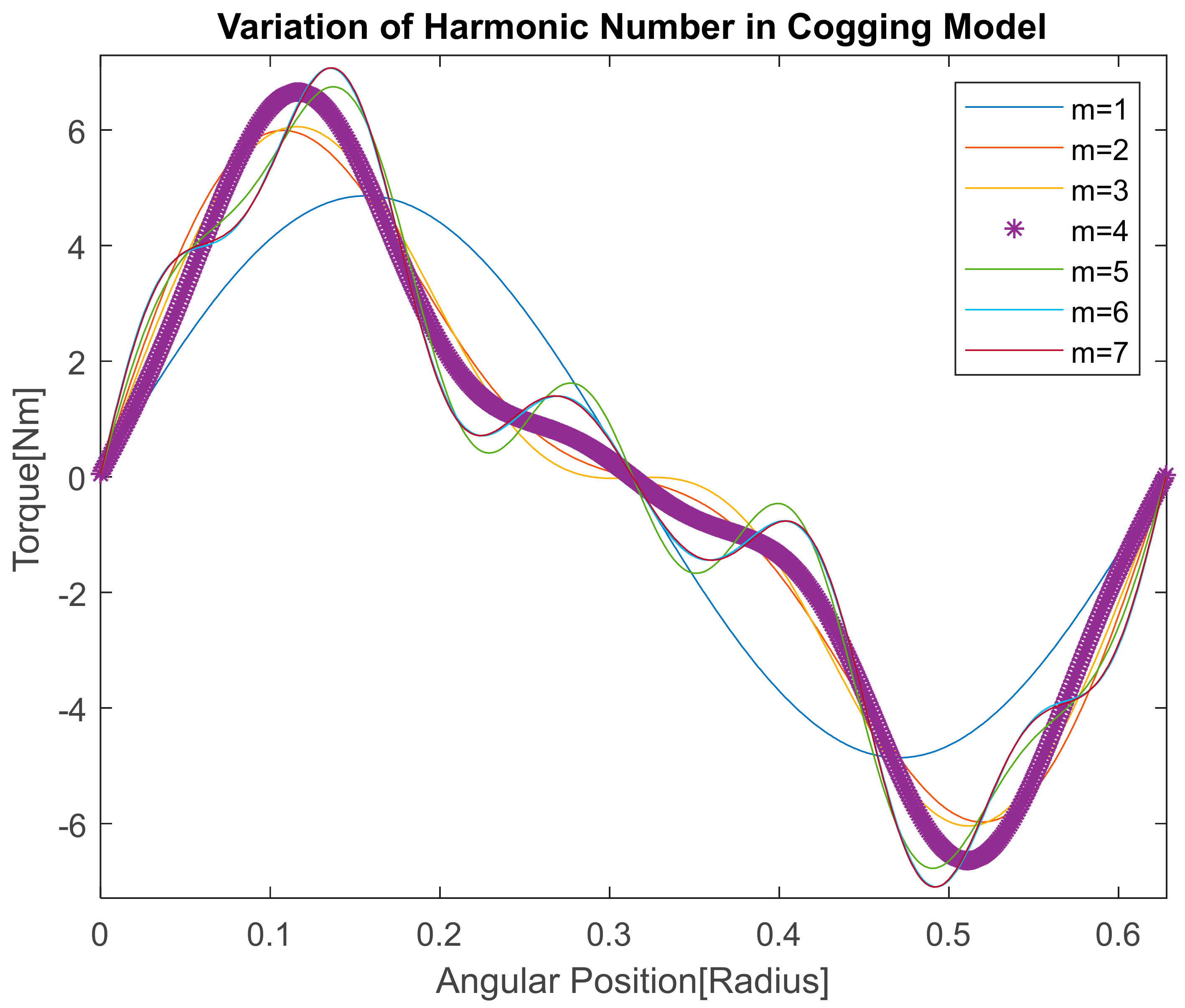
where $T_k$ and the ${\alpha }_k$ are the coefficients of the Fourier harmonic development, Z is the number of stator teeth, ${\vartheta }_m$ is the angular (mechanical) position of the rotor, and m is the number of harmonics that are used to approximate the actual shape of the cogging torque, $T_{cog}$. As reported in Figure 2, we have carried out a simulation analysis and a comparison in terms of variance of the number of harmonics to represent the cogging torque as a function of angular position. The results in Figure 2 show that four harmonics (m = 4) in Equation (1) are sufficient to represent the cogging torque (i.e., a Fourier development with four terms is a good approximation to describe the cogging phenomenon).

The actual values of the coefficients are reported in

Table 1. Cogging torque model parameters.

Coefficient in Equation (1)	Value
$T_1$	$4.85 \mathrm{N}$m
$T_2$	$2.04 \mathrm{N}$m
$T_3$	$0.3 \mathrm{N}$m
$T_4$	$0.06 \mathrm{N}$m
${\alpha }_1$	$0.009 \mathrm{rad}$
${\alpha }_2$	$0.01 \mathrm{rad}$
${\alpha }_3$	$0.017 \mathrm{rad}$
${\alpha }_4$	${\mathsf{\alpha }}_3$

. The values of the coefficients depend on the morphological and magnetic characteristics of the synchronous machine as well as on the magnetic exchange induced to the air gap and the magnetic permeability of the rotor and stator materials.

Table 2. Motor model parameters.

Motor Model Parameter	Value
$R_s$	$3.3 \mathrm{Ohm}$
$L_{eq}$	$50 \mathrm{mH}$
$k_{\varphi }$	$0.5 \mathrm{Wb}$
$J_m$	$0.02{ \mathrm{Kgm}}^2$
$p$	$3$
$\beta$	$0.01 \mathrm{Ns}/\mathrm{m}$

shows the parameters of the considered electrical machine. In Table 2, $R_s$ represents the electrical resistance of the stator’s windings, $L_{eq}$ is the equivalent inductance of the three-phase circuit that represents the dynamics of the electrical part of the machine, $k_{\phi }$ is the intensity of the magnetic flux generated by the permanent magnets, p represents the number of polar pairs, $J_m$ is the motor inertia, and $\beta$ is the friction coefficient.

The parameters shown in Table 1 and Table 2 are relative to an SPM powered by 400 VAC with the features shown in

Table 3. Features of the considered electric motor.

Motor Performance Parameter	Value
Nominal Power	15 kW
Nominal Speed	1500 rpm
Maximum Speed	2000 rpm
Nominal Torque	95.5 Nm
Stall Torque	230 Nm

. In particular, we refer to the brushless motor model Q2CA2215KVXS00M [23], using an inverter model RS1C10AL [24].

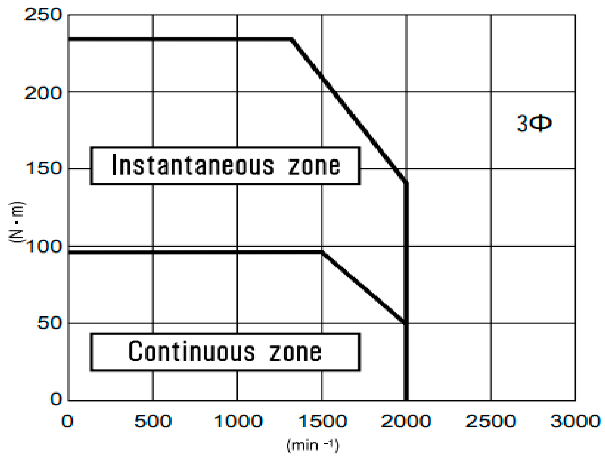
In particular, a motor with the characteristics in Table 3 has a torque–speed curve similar to that shown in Figure 3. In this article, we assume working in the continuous zone of the characteristic reported in Figure 3.

It is worth noting that this work models the presence and effects of the cogging torque in an AC brushless motor with SPM architecture and uses this model in a correction algorithm, but it is not essential to know the internal geometry of the machine in terms of geometrical properties of the permanent magnets and stator caves. This because the most relevant thing is to have a mathematical model of the cogging phenomenon that highlights the dependence of the cogging torque by the rotor position. This model is then inserted into the global model of the drive system.

Instead, the dependence of the cogging torque coefficients shown in Table 1 by the internal geometry of the permanent magnets and stator caves would be needed in a work aiming at a modification of the machine structure, but this is not the case for the present study.

To make more realistic the analysis of the cogging torque reduction by the nonlinear control method proposed, a perturbated version of the cogging mathematical model of Equation (1) is inserted into the model of the mechanical equilibrium. Into the perturbation made by the noise simulation in Figure 4 is inserted the effect of the unavoidable torque ripple caused also by the nonideal commutation of the inverter switching logic. We used the model with four harmonics to project the control laws. In particular, the perturbation on the cogging model is simulated by a white Gaussian noise $w\left(t\right)$, the effects of which can be seen in Figure 4. In particular, in our case, $w\left(t\right)~N\left(\mu ,\sigma \right)$ with $\mu =0 , \sigma =1 Nm$ is inserted.

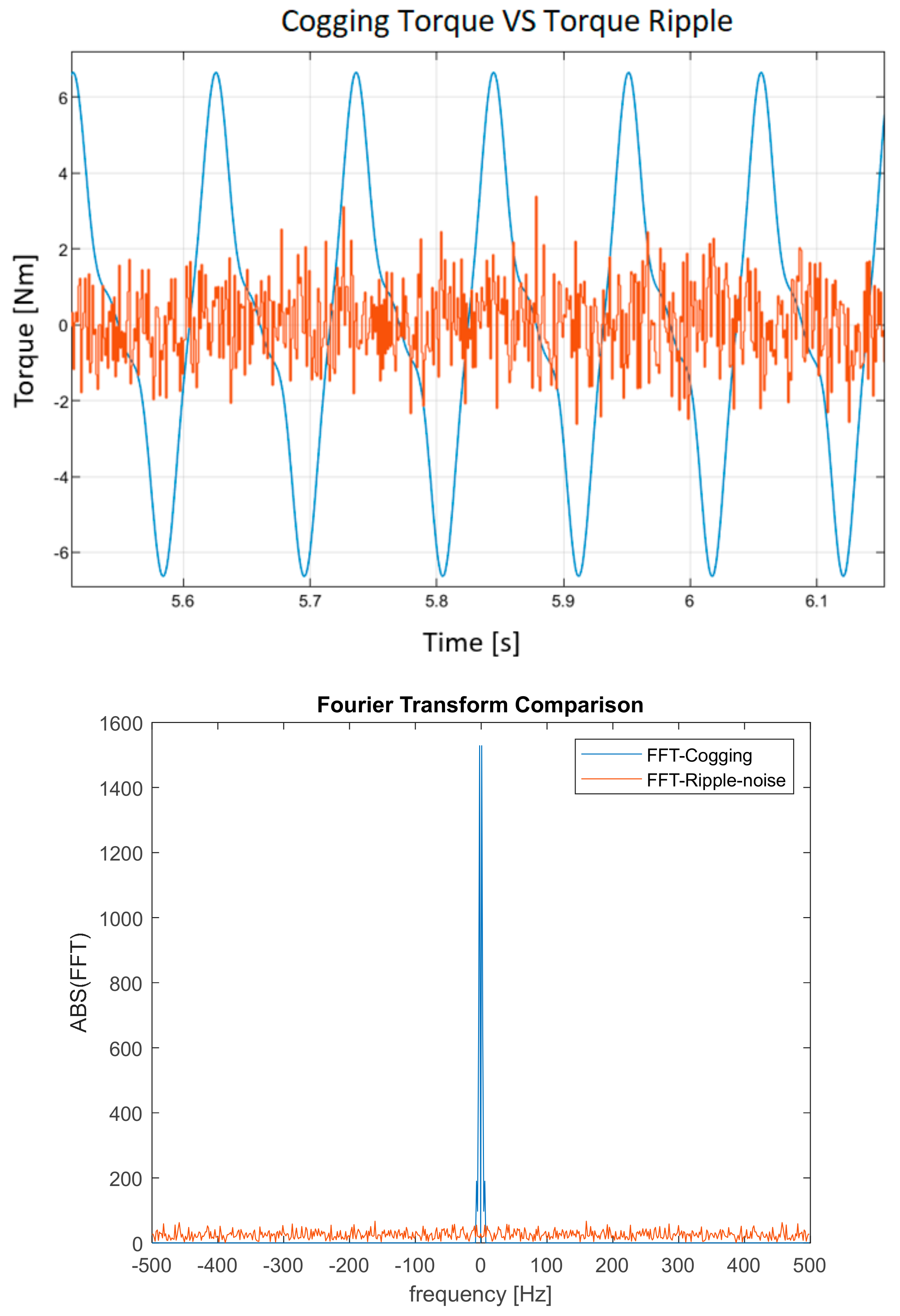
According to other works in the literature, such as [25], a reasonable value of torque ripple is around 10% of the nominal torque, i.e., $\mp 10 Nm$ for a motor with nominal torque of about 100 $Nm$, as shown in Figure 3. In general, torque ripple clearly also includes cogging torque behavior, so in our work, we included the two terms by also adding to the model of Equation (1) the noise term $w\left(t\right).$ To respect the typical percentage of ripple entities, we set an intensity of about $7 Nm$ for the cogging torque, adding a Gaussian noise with $3\sigma =3 Nm$, so the intensity of the torque ripple is $\mathrm{in} \mathrm{the} \mathrm{range} \mp 10 Nm$ ($T_{cog} by model \mp 3\sigma$). To better highlight the comparison of the cogging torque vs. the added torque ripple, modeled as a Gaussian noise contribution, Figure 5 shows the two separated signals—cogging torque in blue and Gaussian-like added torque ripple in red, in the time domain (top) and frequency Fourier transform domain (bottom).

3.2. Brushless Motor Modeling with the Cogging Term

A classical model of a synchronous machine is considered. According to the unified theory of electric machines [26], and after the coordinate transformations necessary to delete the dependence on angular rotor position in electromagnetic torque, we can write the equations of electromechanical equilibrium in the following way:

$$\left[\begin{array}{c}{u}_d\\ u_q\end{array}\right]= \left[\begin{array}{cc}{R}_s& -L_{q}p\frac{d{\vartheta }_m}{dt}\\ L_{d}p\frac{d{\vartheta }_m}{dt}& R_s\end{array}\right]\left[\begin{array}{c}{i}_d\\ i_q\end{array}\right] + \left[\begin{array}{cc}{L}_d& 0\\ 0& L_q\end{array}\right]\left[\begin{array}{c}\frac{d{i}_d}{dt}\\ \frac{d{i}_q}{dt}\end{array}\right] + \left[\begin{array}{c}0\\ p\frac{d{\vartheta }_m}{dt}{k}_{\varphi }\end{array}\right]$$

(2)

$$J_m\frac{d^2{\vartheta }_m}{d{t}^2}+ \beta \frac{d{\vartheta }_m}{dt}=T_{em}+ {\displaystyle \sum }_{k=1}^m{T}_k\sin \left(kZ{\vartheta }_m+ {\alpha }_k\right)+w\left(t\right)$$

(3)

In the above equations, the term of cogging torque is inserted into the mechanical equilibrium as an overlapping effect in the global torque. In Equation (2) $u_d and u_q$ are the voltage components in the d–q frame, $i_d and i_q$ are the current components in the d–q frame, $L_d and L_q$ are the inductance of the equivalent circuit transformed in the d–q frame, ${\vartheta }_m$ is the mechanical angular position, and $T_{em}$ is the electromagnetic torque that in the general case, is given by $T_{em}=\frac{3}{2}p\left[\left(L_q-L_d\right)i_d{i}_q+k_{\phi }{i}_q\right]$. In this work, reference is made on a SPM machine which has the characteristic of having $L_d=L_q=L_{eq}$, i.e., $\frac{L_d}{L_q}=1,$ so that the expression of the electromagnetic torque is given by $T_{em}=\frac{3}{2}p{k}_{\varphi }{i}_q$.

Working with $\frac{L_d}{L_q}=1$ means that the electric machine is considered as an isotropic brushless machine, so there are not configurations of maximum or minimum reluctance and clearly, the inductance values of the equivalent circuits along the direct and quadrature axis (the frame that is obtained after the Park transformation) are equal. Such an assumption has been made for the sake of clarity, as it makes it easier to understand the expression of the electromagnetic torque. However, nothing changes if we consider an anisotropic machine with different L_d and L_q values (typically, L_d << L_q). Moreover, in the paper, we emulate a FOC control where the i_d current is constrained to a zero value, and this implies that the anisotropic behavior does not contribute to the final trajectory tracking result. To include the anisotropic behavior due to arrangement of the magnets in an IPM structure, then the term 3/2·p·(L_q-L_d)·i_d·i_q, which is zero in the case where $L_d=L_q,$ should be included in the ideal electromagnetic torque, i.e., the above-reported T_em term in the mechanical equilibrium in the equations of the dynamic of the electrical machine.

4. Feedback Linearization Control for a Brushless Motor

For convenience in the controller design, the equations in the state form are usually assumed, as shown in Equation (4).

$$\begin{gathered} \dot{x}=\left[\begin{array}{c}{\dot{x}}_1\\ {\dot{x}}_2\\ {\dot{x}}_3\\ {\dot{x}}_4\end{array}\right]=\left[\begin{array}{c}p{x}_4{x}_2-\frac{R_s}{L_{eq}}{x}_1\\ -\frac{1}{L_{eq}}[R_s{x}_2+p{x}_4(L_{eq}{x}_1+k_{\varphi }\left)\right]\\ \frac{1}{J_m}[\frac{3}{2}p{k}_{\varphi }{x}_2-\beta x_4+{\displaystyle \sum _{k=1}^4}{T}_{k}sin(kZ{x}_3+{\alpha }_k)]\end{array}\right]+\left[\begin{array}{c}\frac{1}{L_{eq}}\\ 0\\ 0\\ 0\end{array}\right]u_1+\left[\begin{array}{c}0\\ \frac{1}{L_{eq}}\\ 0\\ 0\end{array}\right]u_2 \\ =f(x)+{\displaystyle \sum _{k=1}^m}{g}_k(x)u_k \end{gathered}$$

(4)

It should be further noted that the state form is nonlinear, but it is “affine in the control” with the classic choice of state variables $x_1=i_d , x_2=i_q ,x_3={\vartheta }_m ,x_4={\dot{\vartheta }}_m$ and control variables $u_1=u_d, u_2=u_q$. The vector field $f\left(x\right)$ is called drift vector while the $g_k\left(x\right)$, with k from 1 to m, are the control vector fields.

Referring to the nonlinear theory of control systems [27], the goal is to design the control law in order to formally obtain a change of state variables that have a linear dynamic in the new base. The operating procedure consists of deriving all the expressions of the outputs for a total number of times necessary to obtain an expression where at least one of the components of the control vector appears.

Calling $y_i=h_i\left(x\right)$ the i-th control output and ${\mu }_i$ the i-th derivation order in which at least one element of the control vector appears, the equations useful for the systematic design of the controller and therefore the change of variables take the following form:

$$\frac{d^{{\mu }_i}}{d{t}^{{\mu }_i}}{y}_i=\frac{{\partial }^{{\mu }_i-1}{h}_i\left(x\right)}{\partial x^{{\mu }_i-1}}\left(f\left(x\right)+{\displaystyle \sum }_{k=1}^m{g}_k\left(x\right)u_k\right)=L_f^{{\mu }_i}{h}_i\left(x\right)+{\displaystyle \sum }_{k=1}^m{L}_{g_k}{L}_f^{{\mu }_i-1}{h}_i{u}_k;\hspace{1em}i=1,2\dots ,l$$

(5)

Inserting the linearization condition by imposing that the i-th derivative is equal to a component of the control vector $v={\left[\begin{array}{ccc}{v}_1& \dots & v_l\end{array}\right]}^T$ for the new base ($y_i^{{\mu }_i}=v_i \forall i$), thus deciding that the linear dynamics emulate a chain of multiple integrators, the following matrix form is obtained:

$$Y^{\mu }=\left[\begin{array}{c}{y}_1^{{\mu }_1}\\ ⋮\\ y_l^{{\mu }_l}\end{array}\right]=\left[\begin{array}{c}{L}_f^{{\mu }_1}{h}_1\\ ⋮\\ L_f^{{\mu }_l}{h}_l\end{array}\right]+\left[\begin{array}{ccc}{L}_{g_1}{L}_f^{{\mu }_1-1}{h}_1& \cdots & L_{g_m}{L}_f^{{\mu }_1-1}{h}_1\\ ⋮& \ddots & ⋮\\ L_{g_m}{L}_f^{{\mu }_l-1}{h}_l& \cdots & L_{g_m}{L}_f^{{\mu }_l-1}{h}_l\end{array}\right]\left[\begin{array}{c}{u}_1\\ ⋮\\ u_m\end{array}\right]=T\left(x\right)+E\left(x\right)u=\left[\begin{array}{c}{v}_1\\ ⋮\\ v_l\end{array}\right]=v$$

(6)

Inverting the equality, the expression for the controller in Equation (7) is obtained:

$$u= E^{+}\left(v-T\right)+\left(I-E^{+}E\right)\tau$$

(7)

A typical choice of the state vector in the new base is the following:

$$z=\left[\begin{array}{c}{z}_1\\ z_2\\ \begin{array}{c}⋮\\ z_{\mu }\end{array}\end{array}\right]=\left[\begin{array}{c}{h}_1\\ ⋮\\ \begin{array}{c}{L}_f^{{\mu }_1-1}{h}_1\\ ⋮\\ \begin{array}{c}{h}_l\\ ⋮\\ L_f^{{\mu }_l-1}{h}_l\end{array}\end{array}\end{array}\right]$$

(8)

In Equation (8), $\mu ={\displaystyle \sum }_k{\mu }_k$ is the relative degree of the system, or rather the total number of derivates that is needed to have at least one component of the control laws vector in the $y_k{}^{{\mu }_k}$ expressions.

In Equations (5) and (6), with $L_f^{{\mu }_i}{h}_i\left(x\right)= \frac{{\partial }^{{\mu }_i}{h}_i\left(x\right)}{\partial x^{{\mu }_i}}f\left(x\right)$, it is indicated the ${\mu }_i$-th Lie derivate of $h_i\left(x\right)$ along the vector field $f\left(x\right)$, and $L_{g_k}{L}_f^{{\mu }_i-1}{h}_i=\frac{\partial }{\partial x}\left(\frac{{\partial }^{{\mu }_i-1}{h}_i\left(x\right)}{\partial x^{{\mu }_i-1}}f\left(x\right)\right)g_k\left(x\right)$ is the Lie derivate along the k-th control vector $g_k\left(x\right)$.

In Equation (7), the vector $\tau$ is an arbitrary vector that is projected in the null space of the matrix $E\left(x\right)$ and is often a function to minimize. It is projected in the null space through the operator $I-E^{+}E$, where $I$ indicates the identity matrix and $E^{+}$ indicates the singular value decomposition of the matrix $E\left(x\right)$. To avoid problems with the projection of the control components in the null space, we assume the case in which the $E\left(x\right)$ matrix is square and invertible. This means that starting from now, we omit the contribution of the vector $\tau$ in Equation (7).

The new controller $v\left(t\right)$ can be chosen with a linear technique that in this context, will be a static feedback of the input status made in the following way:

$$v_i=v_{re{f}_i}+ {\displaystyle \sum }_{j=1}^l{K}_{ij}\left(z_j-z_{re{f}_j}\right)$$

(9)

In Equation (9), $z_j$ is the j-th variable of the state vector in the new base, $K_{ij}$ is a component of the control gain matrix, and $v_{re{f}_i}$ is often used to define a reference on the derivate of the components of the state vector in the new base.

To highlight the potential of this control technique, the angular position control was taken into consideration by comparing it with a classic cascade structure FOC scheme.

For position control, therefore, control outputs $y_1=x_1=i_d , y_2=x_3={\vartheta }_m$ are taken into account; in this way, we obtain the following expressions in terms of the control vector:

$$u_1=L_{eq}{v}_1+R_s{x}_1-p{L}_{eq}{x}_1{x}_2$$

(10)

$$\begin{gathered} u_2= \frac{2J_m{L}_{eq}}{3p{k}_{\varphi }}\left\{-\frac{1}{J_m}\left\{\frac{3p{k}_{\varphi }}{2L_{eq}}\left[-R_s{x}_2-p{x}_4\left(L_{eq}{x}_1+k_{\varphi }\right)\right]+Z{x}_4\left({\displaystyle \sum }_{k=1}^4{T}_k\cos \left(Zk{x}_3+{\alpha }_k\right)\right) \\ -\frac{\beta }{J_m}\left(\frac{3p{k}_{\varphi }{x}_2}{2}+\left({\displaystyle \sum }_{k=1}^4{T}_k\sin \left(Zk{x}_3+{\alpha }_k\right)\right)-\beta x_4\right)\right\}\right\}+\frac{2J_m{L}_{eq}}{3p{k}_{\varphi }}{v}_2 \end{gathered}$$

(11)

This is also the case of exact linearization feedback, because the state vector of the new base has the same dimension of the state of the model in axes d–q. This guarantees the stabilization of the starting system, because three derivations are necessary for $y_2$ and one for $y_1$, which gives us a relative degree of four. This also represents the cardinality of the initial state space.

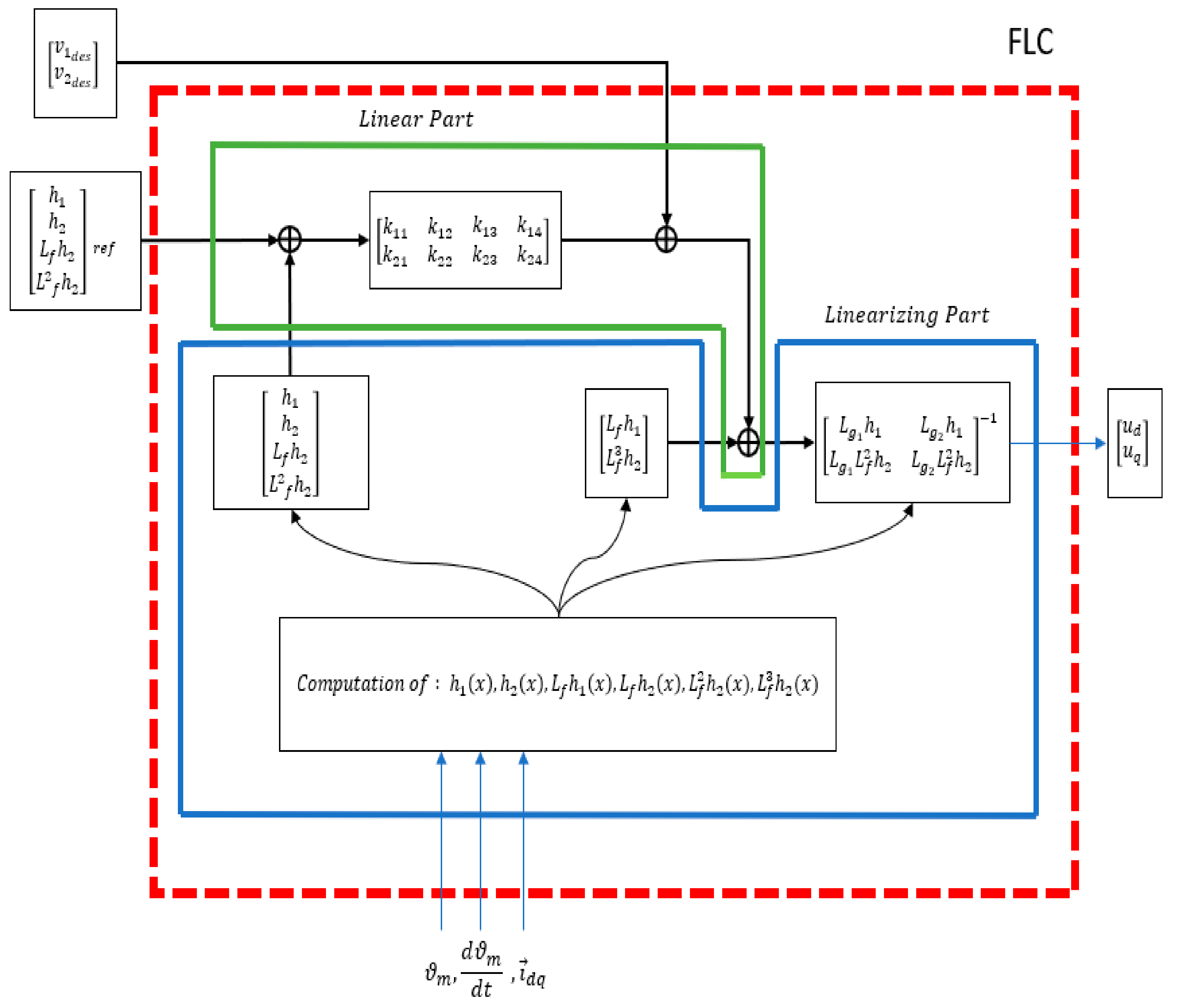
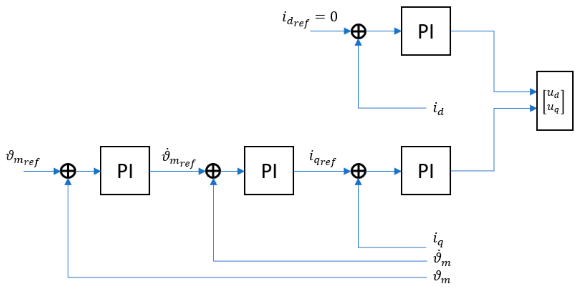
Figure 6 schematically shows the different structure of the nonlinear control system with respect to the classic cascade architecture in Figure 7. In classic cascade architecture is considered the case of PI (proportional-integrative) control for all three concentric loops: two parallel loops for the d–q axis currents, then cascaded to angular speed loop, and angular position loop.

Applying $u_1$ and $u_2$, the dynamic in Equation (12) is obtained, and this representation of the new state dynamic has the property of complete controllability, which guarantees that we can change all the eigenvalue with a state feedback control.

$$\dot{z}=Az+Bv=\left[\begin{array}{cc}\begin{array}{c}0\\ 0\\ 0\end{array}& \begin{array}{ccc}0& 0& 0\\ 0& 1& 0\\ 0& 0& 1\end{array}\\ 0& \begin{array}{ccc}0& 0& 0\end{array}\end{array}\right]z+\left[\begin{array}{cc}1& 0\\ \begin{array}{c}0\\ 0\\ 0\end{array}& \begin{array}{c}0\\ 0\\ 1\end{array}\end{array}\right]v,\hspace{1em}z=\left[\begin{array}{c}{h}_1\\ h_2\\ \begin{array}{c}{L}_f{h}_2\\ L_f^2{h}_2\end{array}\end{array}\right],\hspace{1em}y=Cz=\left[1 1 0 0\right]z$$

(12)

Another advantage of the linearization feedback technique with respect to all the other control techniques is that of being able to also choose non-feedback signals as control outputs; for example, the power for joule effect. The linearization feedback technique also permits choosing a zero-power reference together with a position reference, thus guaranteeing that the change of variables is formally fair for the reasons mentioned above. This allows to constrain the behavior of physical quantities that are the result of the combination of those classically used for feedback (currents and position or angular velocities).

For example, for the “joule power – position” control, we can take into account the output functions $y_1=R_s\left(x_1^2+x_2^2\right), y_2=x_3$, and applying the procedure described above, the following expressions are obtained for $E\left(x\right)$ and $T\left(x\right)$, from which we can obtain the control vector by applying Equation (7).

$$E\left(x\right)=\left[\begin{array}{cc}\frac{2R_s}{L_{eq}}{x}_1& \frac{2R_s}{L_{eq}}{x}_2\\ 0& \frac{2p{k}_{\varphi }}{2J_m{L}_{eq}}\end{array}\right]$$

(13)

$$T\left(x\right)=\left[\begin{array}{c}\frac{2R_s}{L_{eq}}[R_s{x}_2+p{x}_2(L_{eq}{x}_1+k_{\varphi })]x_2-2R_s(p{x}_2{x}_4-\frac{R_s}{L_{eq}}{x}_1)x_1\\ \frac{\beta }{J_m}(\frac{3}{2}p{k}_{\varphi }{x}_1+{\displaystyle \sum _k}{T}_{k}sin(kZ{x}_3+{\alpha }_k)-\beta x_4)-\frac{3p{k}_{\varphi }}{2J_m{L}_{eq}}(R_s{x}_2-p{x}_4(L_{eq}{x}_4+k_{\varphi }))-Z{x}_4{\displaystyle \sum _k}{T}_{k}cos(kZ{x}_4+{\alpha }_k)\end{array}\right]$$

(14)

We can observe that this is another case of exact feedback linearization, because the relative degree for the first output function is one and for the second is still three, as in the previous case.

In the case of current control or angular velocity, this is no longer guaranteed. Therefore, it will be necessary to verify that in the completion of the state vector to satisfy formal issues related to the theorem of the implicit functions, the zero-dynamics criterion is also satisfied.

5. Reducing Cogging Control and Implementation Results

The dynamic model considered for the motor is the one previously presented in Section 4. The model is parametric. For convenience, a mask has been created that encloses all the electric drive parameters. To apply the proposed technique to different electric machines is quite simple, since it is sufficient to change the parameters of the model of the engine in the mask. The parameters that have been used for the motor and for the cogging model to obtain the quantitative results presented in this work are shown in Table 1, Table 2 and Table 3. These parameters are typical of a motor for robotic manipulators for industrial applications. Reference is made to a classical AC motor with SPM structure [23,24]. As reference signals, a zero reference as justified in [26] is chosen for the direct axis curves. Meanwhile, for the position reference, a constant signal with sudden positioning changes at intervals has been selected to simulate a typical situation for a machine used in precision applications, such as, for example, a processing by a computer numerical control (CNC) machine. To make the simulation more realistic, an inverter with a pulse width modulation (PWM) modulator model has been incorporated, where the carrier is a triangular signal with amplitude of 700 V and the frequency is 10 kHz. In the following, we report the results obtained for the problem of tracking the current references in the direct axis and in the rotor angular (mechanical) position. 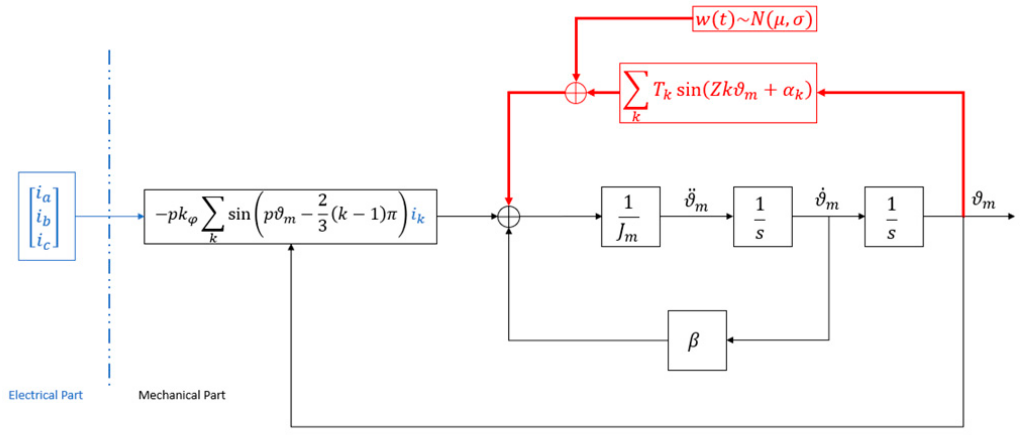Figure 8 shows the scheme of the implementation for the mechanical equilibrium to understand better the inclusion of the cogging term in the SPM model.

It is worth noting that the cogging torque behavior is an intrinsic nonlinearity that is already considered in this work. Other nonlinearities, such as the saturation effects on the current and on the voltage, are also taken into account with the model of the inverter and with a saturation block in the electrical dynamic equilibrium. Instead, concerning the intrinsic behavior of the magnets in terms of hysteresis curve, we assume working in the linear part of the magnetic characteristic.

In the following, we show the results in terms of trajectory tracking control for the angular mechanical position and the current for direct axis frame. The effective advantage of the proposal technique is shown by a comparison with the cascade structure for position control in a FOC structure, as explained in [26].

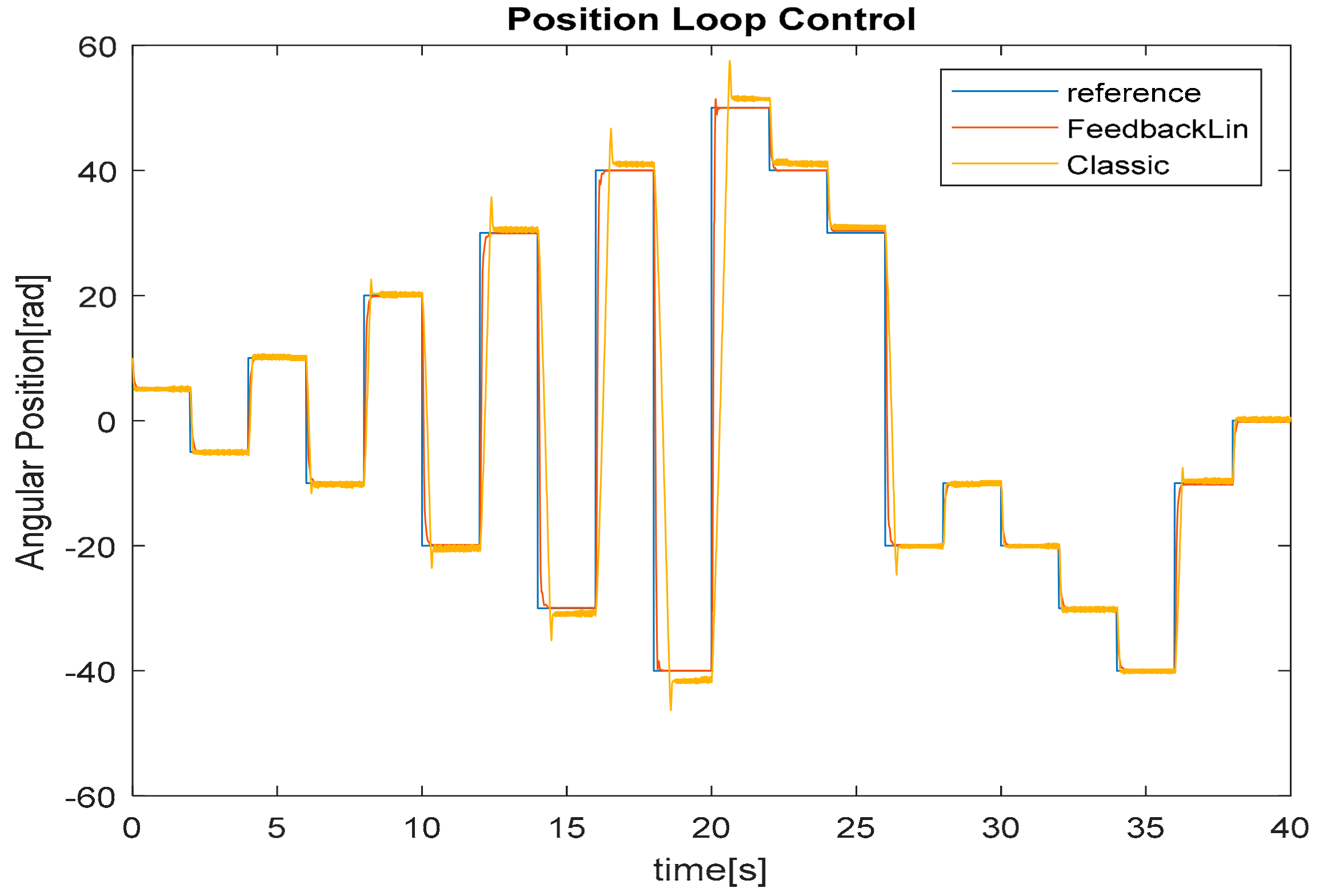
The goal of our work is to propose a method to mitigate the cogging torque effects on the final application (in terms of rotor axis positioning) by the projection of a control laws vector. This means that, differently from other works that propose an alternative design of internal geometry of the machine, we do not aim at deleting the presence of the cogging torque. The effect of our proposed solution can be appreciated in terms of the final result in the path-following problem, where the position, speed, or current in the quadrature axis of the machine is constrained at a precise value by the control system. This is the main difference between the proposed algorithm and classical control techniques, because we directly insert the cogging torque model inside the equations needed for the projection of the control law vector; see Figure 8 and Figure 9.

As previously said, the case of tracking trajectories of constant type has been chosen to simulate the request for rapid change of the angular position, something that often happens in industrial applications such as in automated chains or in robotized cells.

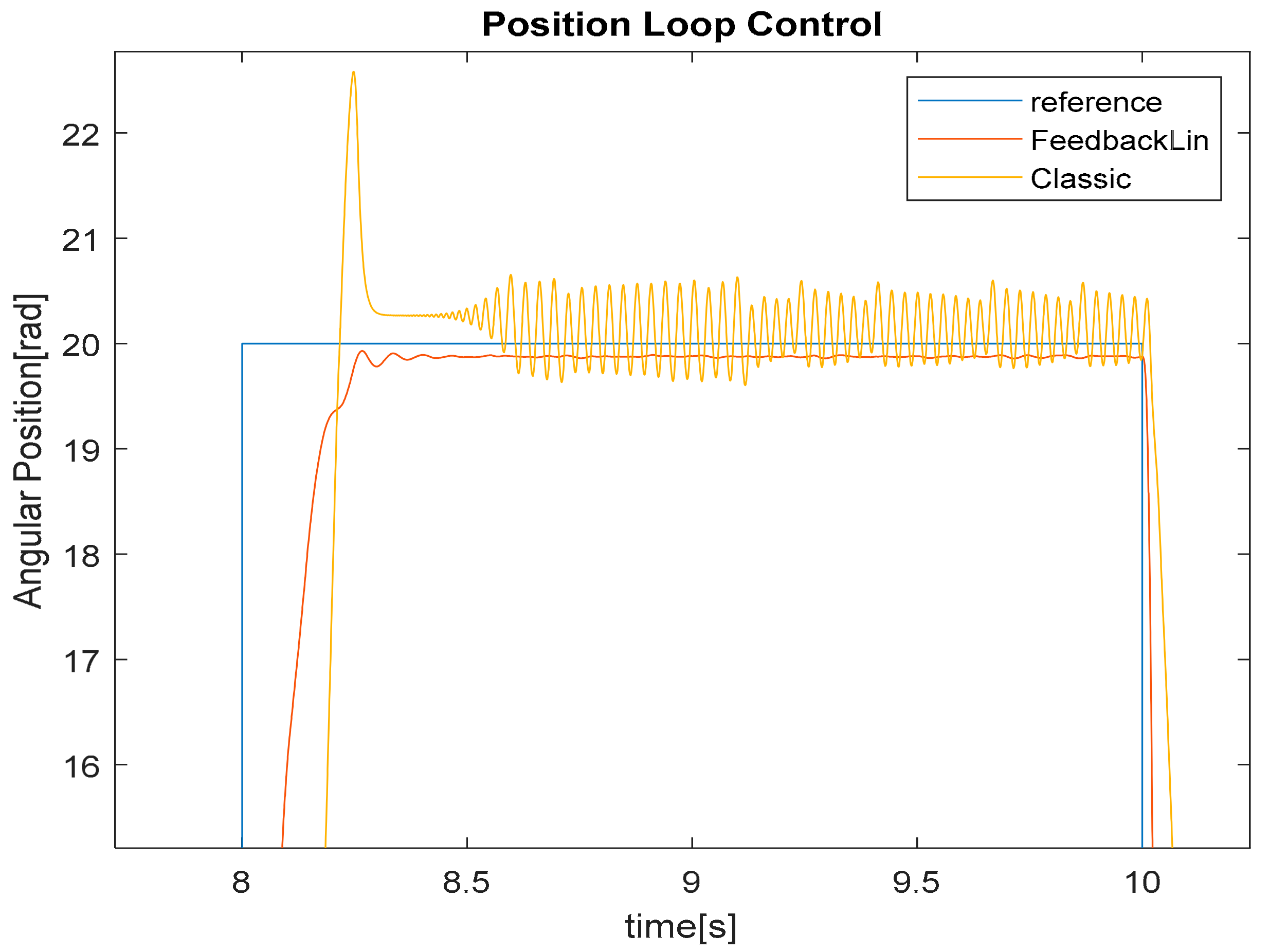
Figure 9 shows the result of the angular position reference tracking. It is shown that nonlinear control is more efficient than the classic cascade architecture in absorbing the oscillation effect due to the cogging torque. Furthermore, the proposed nonlinear control is better than the classic cascade architecture in tracking the reference, due to the fact of exploiting the intrinsic nonlinearities of the model within the control architecture. 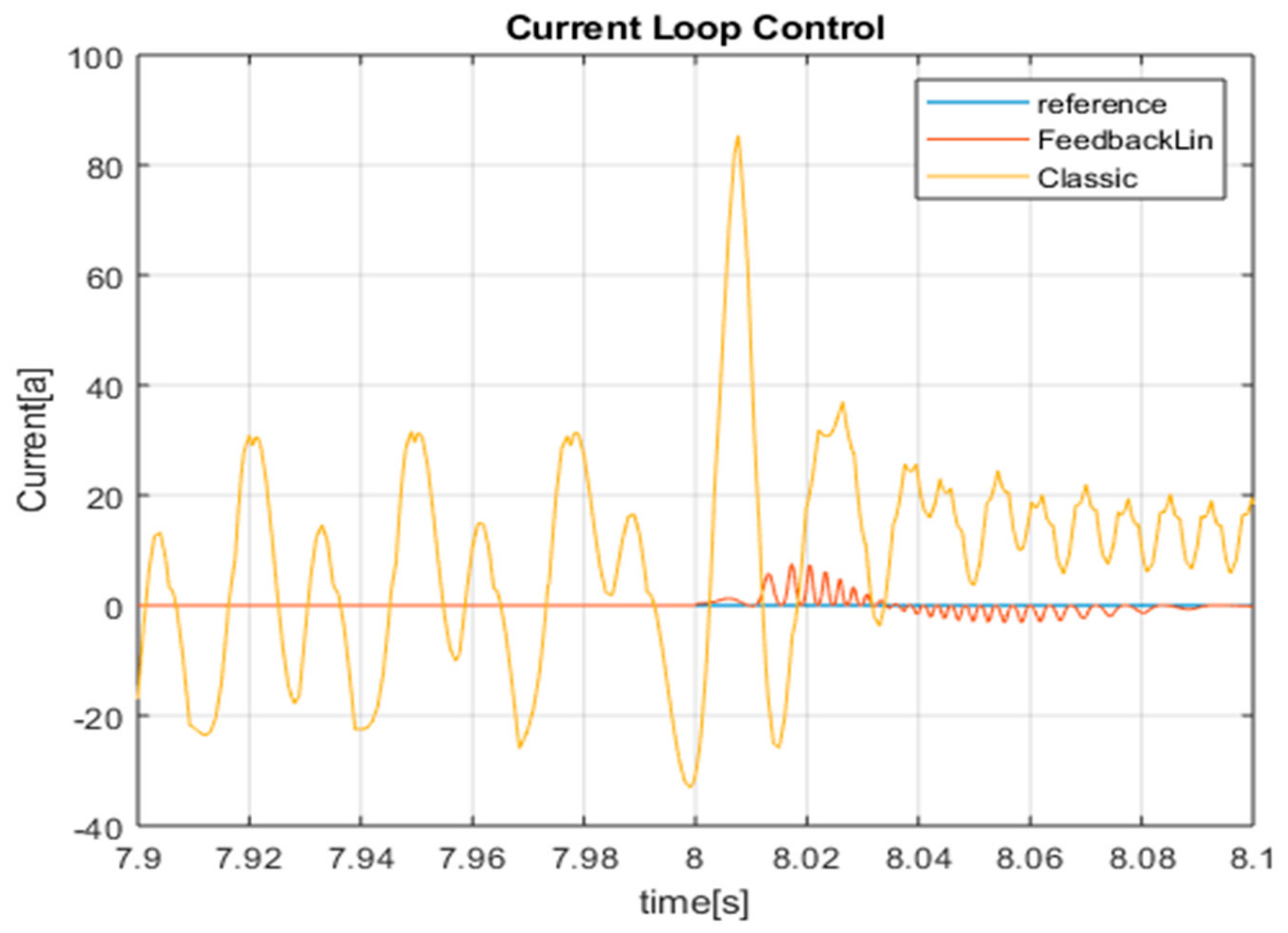Indeed, in Figure 10, when tracking the reference from 8 s to 10 s, the classic cascade control is affected by an overshoot and by oscillations, that instead are avoided when using the proposed FLC technique. Similar results are obtained in terms of current control; see Figure 11.

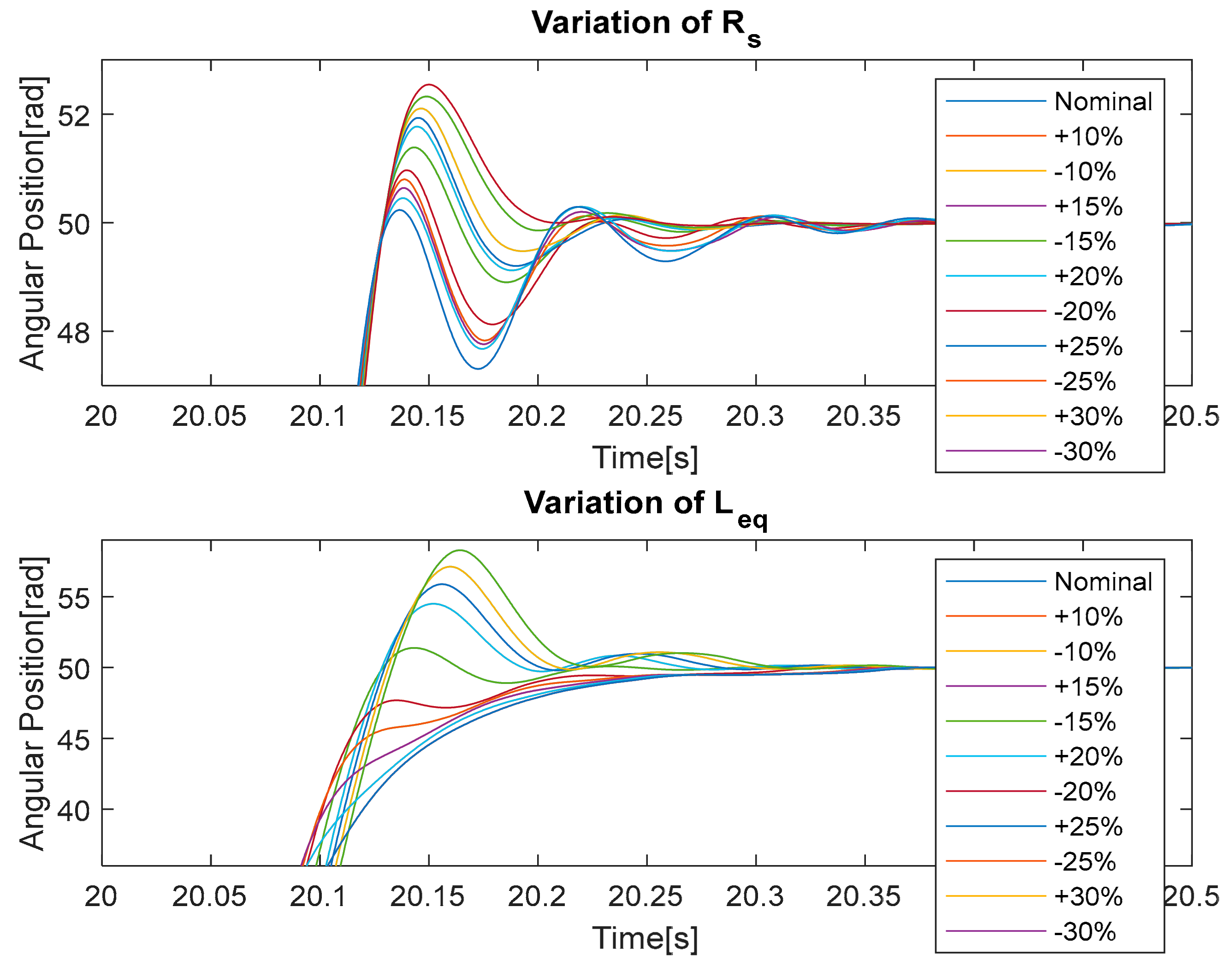
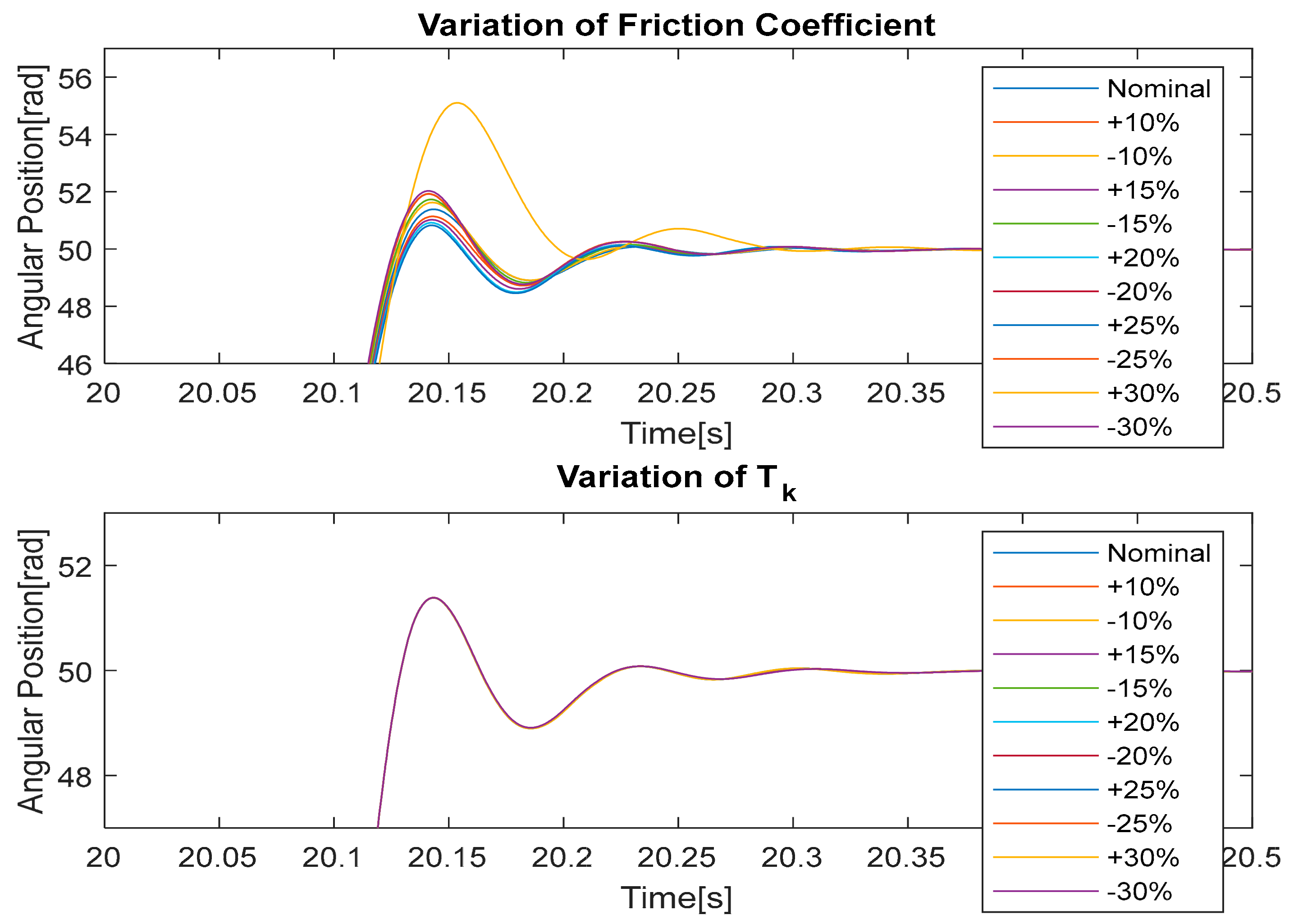
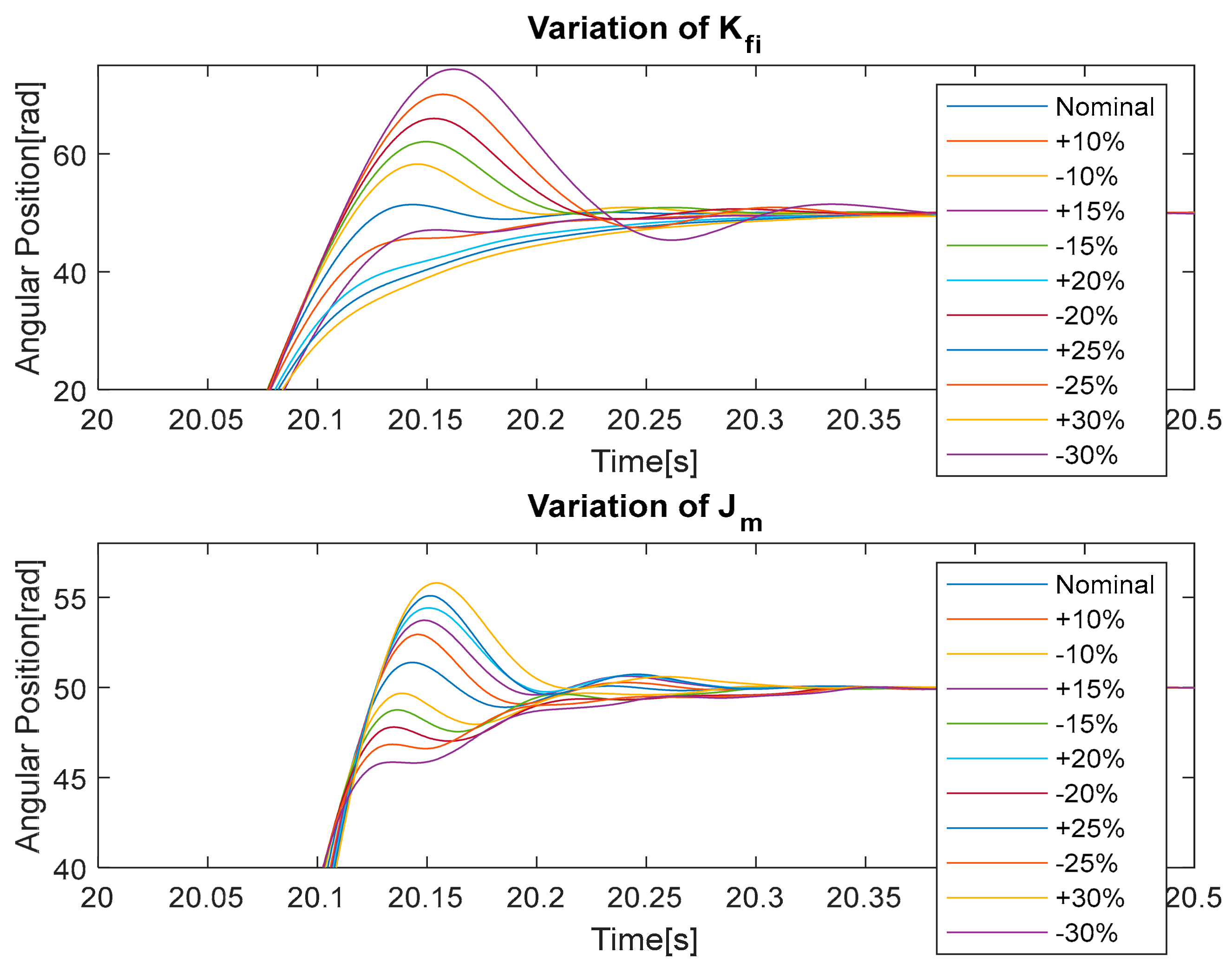
Surely, the control with linearization feedback guarantees a region of asymptotic stability greater than any control based on a linear technique and is therefore more robust to parametric variations. To verify that the proposed control can be applied to a real test bench, we include a graphic analysis of robustness to the variation of the main machine parameters up to ± 30% vs. nominal values considered to design the controller; see Figure 12, Figure 13 and Figure 14.

It must be noted that, apart from the specific case example we have shown, the global model that we use to produce the control laws vector is a scalable model. This means that if the parameters described in Table 1, Table 2 and Table 3 are known, then the proposed algorithm can be applied to all types of synchronous motor, as well as step motors, IPMs, and BLDC (BrushLess DC) motors of all sizes and voltages.

6. Algorithm Profiling and Porting in a Low-Cost Embedded Platform

We have verified the performance of the proposed method using a Simulink profiler (on MATLAB 2018a version release) during the simulation. The profiler collects performance data while simulating the model and generates a report, called a simulation profile, based on the data. The simulation profile generated by the profiler shows how much time Simulink spends executing each function required to simulate the model. The profile helps to determine the parts of the model that require the most time to simulate and hence where to focus the model optimization efforts.

The summary file displays the following performance total; see

Table 4. Description of the fields in the report.

Item	Description
Total Recorded Time	Total time required to simulate the model.
Number of Block Methods	Total number of invocations of block-level functions (e.g., Output()).
Number of Internal Methods	Total number of invocations of system-level functions (e.g., Model Execute).
Number of Nonvirtual Subsystem Methods	Total number of invocations of nonvirtual subsystem functions.
Clock Precision	Precision of the profiler’s time measurement.

.

The summary section then shows summary profiles for each function invoked to simulate the model. For each function listed, the summary profile specifies the information in

Table 5. Description of the fields for the single block.

Item	Description
Name	Name of the Function. This item is a hyperlink. Clicking it displays a detailed profile of this function.
Time	Total time spent executing all invocations of this function on as an absolute value and as a percentage of the total simulation time.
Calls	Number of times this function was invoked.
Time/call	Average time required for each invocation of this function, including the time spent in functions invoked by this function.
Self-Time	Average time required to execute this function, excluding time spent in functions called by this function.
Location	Specifies the block or model executed for which this function is invoked. This item is a hyperlink. Clicking it highlights the corresponding icon in the model diagram. Note that the link works only if you are viewing the profile in the MATLAB help browser.

.

We have compared the performance for both the control structures, with reference to cascade control and proposed FLC, to verify if there is an increase of the complexity that does not justify the adoption of the proposal algorithm.

Table 6. Summary of the Simulink profiler applied to the global Simulink scheme.

Profiler Parameter	Value
Total recorded time	952.69 s
Number of block methods	637
Number of internal methods	8
Number of model methods	11
Number of nonvirtual subsystem methods	32
Clock precision	30 ns
Clock speed	3800 MHz

shows the summary results of the Simulink profiler on the total scheme needed to implement the control (motor model, inverter model, control architecture, input signals generator).

Furthermore, to verify that the profiler is platform-independent, we tried it on two different processors, and we achieved the same results. The testing platforms were an Intel® Core™ i3-6300 CPU @ 3.80 GHz with two cores and an Intel® Core™ i7-8550U CPU @ 1.80 GHz with four cores.

Table 7. Comparison by summary of the profiler.

Algorithm	Time	Calls	Time/Call	Self-Time
FLC	11.953125 1.3%	930736	0.00001284272	7.3593750 0.8%
PI Cascade	11.203125 1.2%	930736	0.00001203685	11.203125 1.2%

shows a comparison in terms of complexity of the FLC and of the Cascade PI controllers, measured as % (1.3% for FLC and 1.2% for PI Cascade) vs. the overall time spent of the whole model according to the Simulink profiler. The results in Table 5 prove that the algorithmic complexity of the FLC technique is similar to that of a classic cascade control. The increasing of complexity is very low compared to the obtained gain in terms of performance in the cogging torque rejection, as proved in Section 5.

In Table 7, the self-time value is lower in the case of nonlinear control, just because is implemented by a MATLAB function that requires a certain amount of time spent to invoke it by the other functions. Meanwhile, this time frame does not exist for the PI control because it is implemented by a native block in Simulink.

Is important to remark that the usage of the Simulink profiler is only helpful to verify the computational cost of our proposed control algorithm with respect to the classical PI controller. This just to decide if it is reasonable or not to implement the nonlinear control technique on a low-cost platform.

To implement the proposed FLC controller on a low-cost embedded system, we exploited the automatic code generation capabilities of Simulink tools. The building procedure from Simulink allows the generation of the code to be embedded in real-time in a low-cost Arduino-Uno platform equipped with the 8-bit microcontroller ATMEGA328 by Atmel, with a clock speed of 16 MHz, a flash memory of 32 KB, a SRAM volatile memory of 2 KB, and an EEPROM non-volatile memory of 1 KB.

Loading the equivalent program of the proposed control algorithm, we have verified that the sketch used 6042 bytes (18%) of the space available for the programs, where the maximum space is 32,256 bytes. The global variables used 226 bytes (11%) of dynamic memory, so 1822 bytes are available for the local variables, where the maximum space is 2048 bytes. Hence, the program and data memory capabilities of a low-cost embedded platform are enough to sustain the proposed control techniques. From a processing point of view, the computational cost of the proposed FLC algorithm when running on the low-cost Arduino-Uno platform is comparable to the computational cost of the classic PI cascade control, as already predicted by the results obtained with the profiler in Table 7.

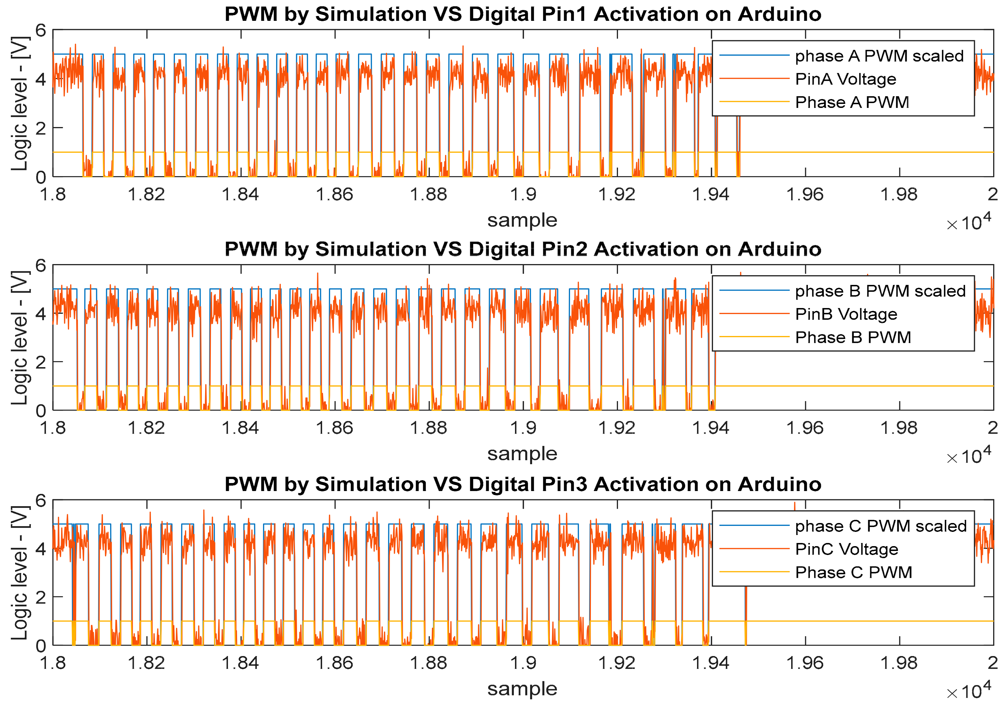
Using a processor-in-the-loop verification approach (i.e., the motor and inverter are modeled and simulated and are interacting with the control algorithm implemented on the target real platform, Arduino-Uno using the ATMEGA328 MCU), Figure 15 presents a comparation between the PWM signal from the full simulated system and the measured signal from the Arduino in the processor-in-the-loop verification testbed. More specifically, Figure 15 shows the voltage measured with an oscilloscope on the three pins of the Arduino for the 3 PWM control phases. This can help in understanding that the low-cost platform is capable to run the control algorithm and to generate the PWM control signals to drive the inverters in the same mode that the simulation has shown. In Figure 15, it is important to notice that the signal in blue is logical (zero or one), since it is the result of the PWM operation by a state machine in the Simulink scheme. Instead, the red signal is the measurement of the physical level, so is an analog signal in the range 0–5 V.

7. Conclusions and Future Work

In this work, a method for mitigating the effects of the cogging torque in permanent magnet synchronous motors has been presented by means of a control technique based on a feedback linearization strategy. The idea is presenting a valid alternative to the techniques of reduction of this phenomenon through physical modifications of the machine, which are expensive. The proposed nonlinear control algorithm is deterministic and easy to derive. This technique allows us to choose which are the control outputs from which to obtain the change of variables. This makes possible to emulate a FOC or DTC control technique; for example, choosing the current and speed or position as outputs. Moreover, the proposed approach allows references to be made in terms of their composition, such as choosing the power for joule effect, control output, and designing $u_1$ and $u_2$ incorporating a power feedback due to the change of base. Instead, this is not possible with a classical cascade control structure that moreover has less ability to reject the cogging effect as it does not exploit its formulation. A comparison between the proposed technique and a cascade control was proposed to show the advantages in mitigating the effect of cogging torque, with reference to a commercial motor. In addition, a parametric robustness analysis was presented to confirm the choice of the proposed control technique for the resolution of the cogging torque problem. Given the good results obtained, a future development could be the development of a sensorless-type architecture. Another future investigation in sensorless application could be to choose the best type of estimator of the state through comparative analysis, including, for example, machine learning techniques, given the increasingly frequent application of the latter.

The analysis through the Simulink profiler confirms that the complexity of the proposed control algorithm is very low. This means that it is reasonable to port the algorithm on different platforms, such as an Arduino unit with an 8-bit ATMEGA328 microcontroller.