Abstract
Conventional parameter designs of two-stage grid-connected photovoltaic (PV) system relied on its mathematical model of the cascade structure (CS), but the procedure is excessively cumbersome to implement. Besides, for a two-stage converter system, the coupling interaction between the power converters can directly lead to a poor parameter design. To overcome this drawback, this paper uses a simplified structure (SS) of single-phase two-stage grid-connected PV system to better design the parameters of the front-stage dc-dc converter. After establishing the small-signal model for SS and CS in the PV system, the relative eigenvalue sensitivity is used as the criterion for judging the influence of some parameters on the stability of the two structures. The stable boundary of MPPT control parameters is compared and discussed in SS and CS, respectively. In addition, the relationship between the front-stage dc-dc converter and the rear-stage dc-ac inverter is analyzed by the modal participation factor calculated in CS. An experiment is also performed at the end of this paper to further verify the feasibility of using SS to design the parameters of the dc-dc converter in the PV system.
1. Introduction
Renewable energy sources, such as wind and solar energy, have begun to replace traditional energy sources as the main source of energy supply in many countries. With the decreasing cost of photovoltaic (PV) modules [1] and the growing utilization rate of the PV cells [2], the application of PV systems has greatly expanded. Compared with the centralized inverter for the high-power PV grid-connected system, the micro-inverter has some certain advantages, such as reducing the cost and ensuring working at the maximum power point, for low power distributed grid-connected PV systems. According to the arrangements and structural characteristics of the dc bus, the topology of the micro-inverter can be roughly categorized into three types, namely, a cascade converter with a dc bus, an inverter with a pseudo dc bus, and an inverter without a dc bus [3]. Furthermore, these structures involve various types of converters, including the Boost converter, Buck-Boost converter [4,5], Flyback converter [6], and resonant push-pull dc-dc converter [7]. Power electronic converter is an inherently strong nonlinear system and it presents various nonlinear phenomena [8,9,10]. Thus, in order to design the circuit parameters and control parameters of the PV system, it is necessary to establish the explicit model and analyze its stability.
At present, the small-signal method is usually employed to establish an effective model to analyze the PV power generation system. Wang et al. [11] introduced the small-signal model of the photovoltaic power generation system in the island operation mode. In [12], the small-signal model of the multi-machine power system with photovoltaic power station is used to study the influence of the low-frequency oscillation of the PV system. It is pointed out that the accessing location and capacity of PV power plant system seriously affects the damping characteristics of the system. Ref. [13] investigated the influence of inverter controller parameters and photovoltaic array structure on the oscillation frequency and damping ratio in large-scale photovoltaic grid-connected power generation systems. Moreover, the maximum power point tracking (MPPT) control is a research hotspot in photovoltaic systems [14,15,16].
The two-stage PV system is a typical grid-connected PV system. Since the solar panel often provides low level dc voltage in PV systems [1], the first stage is typically a dc-dc converter for amplifying voltage and extracting electrical energy from the PV array, and the second stage is a dc-ac inverter for delivering electrical energy to the utility grid. Distributed PV grid-connected power generation system can usually be divided into two energy conversion stages, which interact with each other to make them exhibit more complex characteristics than the system with a single stage [17,18,19].
An observer-model was proposed based on Parker transform to analyze the stability of the single-phase two-stage grid-connected PV system [20], and it can effectively analyze the low-frequency oscillation phenomenon existing on the system. However, cascade structure (CS) is still inseparable from the PV system with dc buses to establish an observer-model. In this case, the coupling relationship between parameters may be difficult to determine [21]. Consequently, it is often complicated to design the parameters of the front-stage dc-dc converter as well as to analyze the stability of the PV system.
To simplify the parameter design of two-stage PV system, this paper uses a simplified structure (SS) to substitute CS for the stability analysis of the front-stage Boost converter. The front-stage converter with boost function, such as Boost converter and Flyback converter, can be used to construct SS for two-stage PV system analysis by replacing the dc bus with a voltage source. This paper uses a Boost converter as the front-stage dc-dc converter to expand the discussion. To obtain the relationship between the two structures in terms of stability, the effectiveness of different parameters in dc-dc converter for SS and CS stability needed to find out, including the capacitance and inductance of the Boost converter and the control parameters of the MPPT controller.
So far, there have been attempted to analyze how the parameters affect dynamic performance. The eigenvalue sensitivity is used to analyze the trend of the system eigenvalues when the controller parameters changed [22]. Furthermore, it is pointed out that the parameters of MPPT controller and inner current control loop seriously affect the stability of the system. In [23], the research focus on the connection between the dc-dc converter and dc bus capacitance in the cascade converter, which has found that the dc bus capacitance has a significant effect on the frequency of the oscillation mode.
This paper is structured as follows. Section 2 describes the mathematics model of proposed SS of two-stage PV system with the small-signal model. In Section 3, relative eigenvalue analysis is employed to study the stability of SS under different MPPT control parameters. And, its dynamics frequency characteristics are described through root locus. In Section 4, the feasibility of SS is verified through comparing the stable boundary of SS with that of CS in different parameter domain of MPPT controller. Furthermore, modal participation factor is introduced to expound the relationship between SS and CS. The experimental result is presented in Section 5, and Section 6 concludes this paper.
2. SS with MPPT Control
The topology illustrated in Figure 1 is based on the traditional cascade structure of two-stage PV system. Considering PV system is actually under the weak grid condition, the LC circuit can be used as the output signal filter [24] and the power grid is equivalent to a voltage source connected with an impedance [25]. The dc-dc conversion stage in Figure 1 uses a Boost converter. Since the dc bus voltage is kept near the rated voltage with the control of the dc-ac inverter [8,26], the output voltage of the dc-dc Boost converter is considered to be constant voltage source in this paper. Based on the criterion that dc bus voltage ripple is kept within a certain control range, SS with MPPT controller is shown in Figure 2, in which Cin and Lb are the input filter capacitor and the energy storage inductance, respectively, and the equivalent series resistance (ESR) of Cin is represented by RCin, RLb is the winding series resistance of Lb.
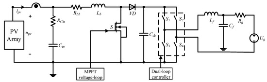
Figure 1.
Cascade structure of a Two-Stage Grid-Connected photovoltaic (PV) system.
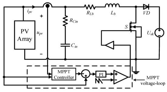
Figure 2.
Schematic diagram of simplified structure of Two-Stage Grid-Connected PV system.
To analyze the stability of SS, a suitable mathematical model must be established. Since the parameters of open circuit voltage UOC, short-circuit current ISC, maximum power point voltage UM and current IM are usually provided in the data sheet of PV array, the fitting model [27] to describe the nonlinear relationship between PV array output current ipv and voltage upv are employed in this research. The PV array model can be expressed as
Here, expansion Equation (1) at maximum power point, it can be calculated that , .
Suppose the system is always operating in continuous current mode (CCM). Using the state space averaging method, the averaged equations corresponding to Figure 2 can be derived as follows
where db is the duty cycle of the power switch in the dc-dc converter.
Since the applicable scope of the transfer function is defined as a linear time-invariant system, the linearization of Equation (1) at the maximum power point is
Marking the steady state values of uCin and iLb at maximum power point as UCin and ILb, respectively. Then, adding small signal disturbance to the steady-state value and ignoring the steady-state quantity, Equation (2) can be expressed as follows after performing the Laplace transform.
Here, , , , and are all the small disturbance signal.
Thus, the open-loop transfer function from the control input to the PV array output voltage can be derived as
where the denominator coefficients are , and .
In general, a classical Boost converter using small-signal model in CCM reveals that its Gvd(s) contains two real zeros in the S-plane [28]. One is a left half plane zero (LPHZ) due to the parasitic capacitance resistance, another is a right-half-plane zero (RPHZ) being peculiar to Boost topology, which is related to filter inductance, load resistance, and duty cycle. As shown in Equation (5), when the dc bus capacitance can be replaced by a constant voltage source, a stable zero is retained in SS and the RPHZ is eliminated. Since dc-dc Boost converter is connected to a dc-ac inverter in the two-stage PV system, SS is used as the basis of subsequent analysis.
3. Stability Analysis of SS
3.1. Parameter Design
The PV array parameters in SS are shown in Table 1. As usual, the duty cycle db is set as 0.5. So, the dc bus rated voltage Udc can be inferred to be 36 V. To meet the requirement both of efficiency and noise interference, the switching frequency fs of the dc-dc converter is set at 20 kHz.

Table 1.
PV Array Parameters.
The function of the input filter capacitor Cin is to reduce the fluctuation of the voltage upv in the PV array, which improves the output efficiency of the PV array.
The value of the inductor Lb in the Boost converter should be able to ensure that the inductor current ripple is limited to a reasonable range. The inductor current ripple rate is 20%, and the inductance value can be calculated by
this paper takes Lb as 2 mH in consideration of a certain margin.
Furthermore, the ripple of upv can be expressed as [1]
In order to maintain the output power of the photovoltaic cell above 98% of the maximum power, the voltage ripple Δupv should be less than 8.5% of the maximum power point voltage [29]. Here, we set Δupv = 0.1% to make SS more accurate in stability analysis as voltage-source replace the bus capacitor, thus obtaining
Cin is taken as 330 μF in consideration of a certain margin.
The parameter value of the proportional integral (PI) controller in the MPPT voltage loop shown in Figure 2 is determined by the Equation (5). With Kp1 = 0.11 and Ti1 = 0.01, the crossover frequency of the open loop fc is set approximately at 500 Hz, and bode diagram is shown in the Figure 3.
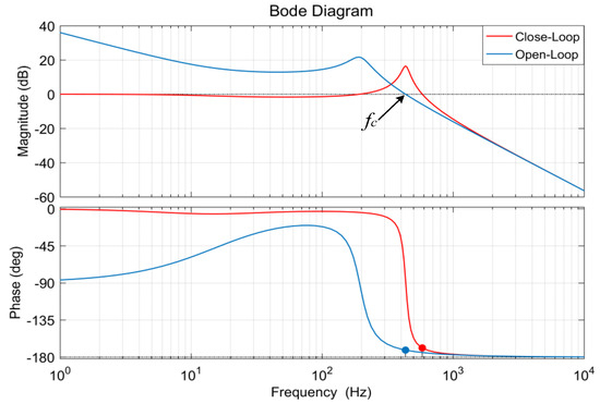
Figure 3.
Maximum power point tracking (MPPT) Voltage-Loop Bode Diagram.
3.2. Stability
Let the MPPT controller variable xmppt be
and duty cycle db can be expressed as
where Kp1 and Ti1 are the gain and time constants of PI controller in the MPPT voltage loop, respectively.
The state variable is denoted by xboost = [uCin, iLb, xmppt]T. Furthermore, Equations (1), (2), (9), and (10) can be joint to obtain the state-space average model of SS
To study the effect of MPPT controller parameters on the stability of SS, both of RCin and RLb are ignored for simplicity. Let the differential term be zero in Equation (11), and the equilibrium point xe can be obtained. Then, putting Taylor expansion of the state-space average model near xe and evaluating Equation (12) under first approximation according to Lyapunov method, small-signal model = AboostΔxboost can be obtained, and
is the Jacobian matrix. Where A11 = , A12 =, A21 =+, A23 =, A31 = 1. So, the eigenvalue λ of the small signal model can be solved
where I represent the unit matrix.
It may be noted that, for every value of Kp1 and Ti1, the system contains a real eigenvalue λ1 and a pair of conjugate eigenvalues λ2,3, which means it involves one oscillating mode and one attenuation mode. For the eigenvalue of the conjugate complex pair σ±jω, the damping ratio of the system oscillation mode can be defined as
The indicator ξ can be utilized to characterize the degree of stability of the oscillating mode. To better analyze the influence of the MPPT control parameters on the stability of SS, the eigenvalues and the damping ratio of the oscillating mode under five different examples are given in Table 2.
Table 2.
Eigenvalues, the damping ratio, and stability margin of the five sets examples of MPPT control parameters in simplified structure (SS).
As the real part of λ2,3 enter into the right half plane of the S-plane in Example-2, Example-4, and Example-5, ξ changes into a negative and in the meanwhile gain margin (GM) and phase margin (PM) are both less than zero. Therefore, the system works in an unstable state at that time and the unstable phenomenon is represented by the low-frequency oscillation of the voltage and current.
Remaining Kp1 is unchanged at Example-1 and Example-2, it can be observed that the decreasing of Ti1 will lead λ2,3 move to the right half plane, which reduces the stability of the system. Let Ti1 = 0.01 at Example-1 and Example-3, the increasing of Kp1 causes λ2,3 to move the right half plane and λ1 to move to the left half plane. Besides, the PM of Example-1 and Example-3 are 8.56° and 14.8° respectively, which means that the stability in Example-3 is actually stronger than the stability in Example-1.
Along with practical application, it is usually found that one or several parameters have a dominant influence on a particular mode of the system, while other parameters take little or no impact. Since multiple circuit parameters exist on the converter, relative eigenvalue sensitivity is used here to evaluate the trajectory alteration when the system parameters changed [22].
To obtain the eigenvalue sensitivity, it is possible to screen for parameters that have an important influence on system stability. Let be the left eigenmatrix of the state matrix A, let be the right eigenmatrix of the state matrix A, and Λ be the diagonal matrix composed of the eigenvalues of the state matrix A. Hence, their relationship can be expressed as
Thus, the eigenvalue sensitivity can be defined as
where λi is the ith eigenvalue of the feature matrix A, and α is a certain system parameter.
The first-order eigenvalue sensitivity of SS is given in Table 3 and it could be found that the sensitivity values of various parameters are significantly different due to the difference in parameter units. To address this problem, the concept of relative eigenvalue sensitivity is introduced to identity such differentiation between parameters.
Table 3.
Eigenvalue sensitivity of different parameters in SS.
It should be noted that the real part of the eigenvalue can clearly reflect the change of the state. For this reason, the relative eigenvalue sensitivity is defined only for the real part of the eigenvalue to simplify the analysis, and then Equation (16) can be replaced by
where RSRe(λi) reflects the impact of relative parameters changing.
Table 4 gives the relative eigenvalue sensitivity of the four key parameters of SS. Furthermore, Figure 4 and Figure 5 depict the eigenvalue locus as the parameters changing. As shown in Table 4 and Figure 4, when RSRe(λi) is positive, eigenvalue locus moves toward the imaginary axis as the parameters increasing. And when RSRe(λi) is negative, eigenvalue locus moves away from the imaginary axis as the parameters increasing. From Figure 5a,b either Ti1 is increasing or Kp1 is decreasing, and the real part of λ1 is increasing. However, the system is still stable, because the real eigenvalue is always less than 0. Furthermore, the reduction of Ti1 and the increasing of Cin will make the real part of the oscillating mode λ2,3 move from the left half plane into the right half plane shown in Figure 4a,c and Figure 5a,c. So, the system tends to be unstable along with the Hopf bifurcation. In addition, the effect of Lb on the stability of the system is almost negligible, which is consistent with the analysis of the relative eigenvalue sensitivity of Lb in Table 4.
Table 4.
Relative eigenvalue sensitivity of different parameters in SS.
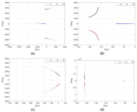
Figure 4.
Loci of eigenvalue λ1, λ2, λ3 as the changing of (a) Ti1; (b) Kp1; (c) Cin; (d) Lb.
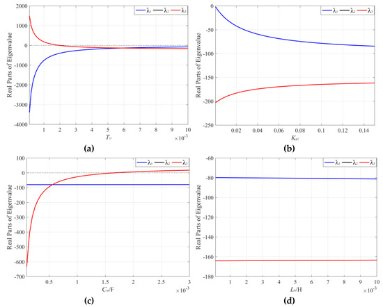
Figure 5.
Trajectory of the real part of λ1, λ2, λ3 as the changing of (a) Ti1; (b) Kp1; (c) Cin; (d) Lb.
4. Comparison of Stability Analysis between CS and SS
4.1. Stable Boundary
In this section, the model of PV grid-connected CS introduced in [20] is used, and then the stable boundary of SS and CS are compared. The parameters of the PV array and the converter are shown in Table 1 and Table 5, respectively.
Table 5.
Converter parameters.
Simulating the circuit of CS circuit, in which MPPT control parameters are assigned according to Example-2 and Example-4 shown in Table 2, respectively. The time domain waveform diagram of the PV voltage upv can be seen in Figure 6, and the corresponding fast fourier transform (FFT) analysis diagram is presented in Figure 7. A large peak amplitude appears at the low-frequency oscillation 422.9 Hz and 325.7 Hz of Example-2 and Example-4 respectively in Figure 7, which is roughly the same as the calculated oscillation frequencies of 443.38 Hz and 332.51 Hz shown in Table 2. Therefore, consistent with the stability analysis of SS, low-frequency oscillation occurs in CS when the parameter in Example-2 and Example-4 are adopted. It indicates that the system is in an unstable state.
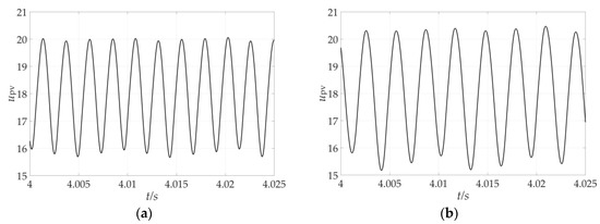
Figure 6.
Waveform of upv when (a) Kp1 = 0.11, Ti1 = 0.001; (b) Kp1 = 0.05, Ti1 = 0.001.
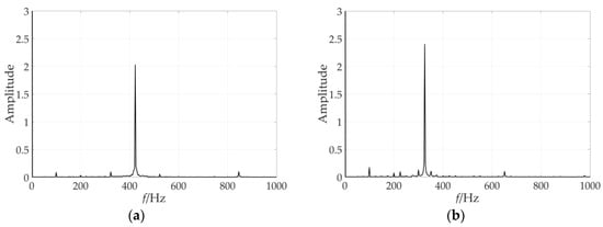
Figure 7.
FFT spectrogram of upv when (a) Kp1 = 0.11, Ti1 = 0.001; (b) Kp1 = 0.05, Ti1 = 0.001.
Next, to further investigate the similarity of the stability of the two structures, Figure 8 depicts the stable boundary of SS and CS with respect to the parameter regions of Kp1 and Ti1. It reveals that the almost same results of the stability analysis described in Section 3 are obtained. Besides, two parameter stability domains of SS are almost identical with CS, and just slight differences exist in the vicinity of the boundary. Thus, it can be concluded that the stability analysis of the dc-dc converter in CS can be carried out in SS.
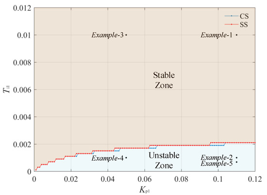
Figure 8.
Comparison of stable boundary between SS and cascade structure (CS).
4.2. Connection and Distinction of SS and CS
According to the method mentioned in Section 3, the relative eigenvalue sensitivity of CS is obtained in Table 6.
Table 6.
Relative eigenvalue sensitivity of different parameters in CS 1.
From Table 6, its influence on different oscillation modes is different for one parameter. For example, the most influential parameter of oscillation mode λ6,7 is Cin, Kp1, and Ti1 have the greatest influence on the attenuation mode λ8. Compared with Table 4, it can be found that λ8 and λ6,7 in CS are analogous to λ1 and λ2,3 in SS, respectively. So, it means the performance of Cin, Kp1, and Ti1 are almost identical in the two structures.
In the small disturbance analysis method, the eigenvalue analysis can judge the stability of the system. However, the eigenvalue is based on the analysis performed at steady-state. To analyze the correlation between the state variables of SS and CS under the transient condition after the disturbance completed, the modal participation factor of the state variable is introduced.
According to the nature of the eigenvalues, each eigenvalue corresponds to a modality of the system. The real eigenvalue corresponds to the attenuation mode of the system, and the conjugate complex eigenvalue corresponds to the oscillating mode. Among the basic modal listed in Table 6, there are three attenuation modes λ1, λ8, and λ9 and four oscillation modes λ2,3, λ4,5, λ6,7, and λ10,11, which play a decisive role in the dynamic behavior of the system. In addition, λ10,11 is independent of the stability of the system due to the introduction of virtual state variables, and it is also independent of the inherent characteristics of the system.
The modal participation factor is a measure that combines the left and right eigenvectors as the degree of interaction between the state variables and the modalities. The correlation between the kth state variable to the ith mode can be represented by a modal participation factor [30] as follows
where represents the kth element of the row vector ; represents the kth element of the column vector . Pki describes the scale of the effect of the ith mode and the kth state variable in the case of the kth state variable is under unit perturbation.
Equation (18) indicates that the modal participation factor is only related to the structural parameters of the system. And it has nothing to do with the disturbance, which is similar to the property of the sensitivity of the eigenvalue. The modal participation factors of the system are given in Table 7. It can be seen clearly that the attenuation mode λ1 is mainly related to the voltage deviation signal ue of the voltage outer loop, the oscillation modes λ2,3 and λ4,5 are mainly related to io and uc2, the oscillation mode λ6,7 is mainly related to iLb and uc1,the attenuation mode λ8 is mainly related to uCin and uc1, the attenuation mode λ9 is mainly related to udc, and the undamped oscillation mode λ10,11 is only related to the constructed virtual state variables g1 and g2. According to the modal participation factor of the system, the basic mode closely related to a certain state variable of the system can be known, thereby a certain state of the system can be affected by regulating the basic mode. Additionally, the nonlinear interaction between the front-stage dc-dc converter and the rear-stage dc-ac inverter can be found through modal participation factor. In Table 7, the corresponding three state variables of SS are uCin, iLb, and uc1. Based on the above analysis, uCin, iLb, and uc1 are the main state variables affecting λ6,7 and λ8. However, they also play almost no effect on the other modes, which indicates that parameters of the front-stage converter designed by SS will not adversely affect the rear-stage inverter in CS.
Table 7.
Modal participation factors of state variables in CS 1.
5. Experiment Verification
To experimentally evaluate the consistency of the stability analysis of the PV system in SS, an experimental setup is implemented as shown in Figure 9. The parameters are consistent with Table 1 and Table 5.
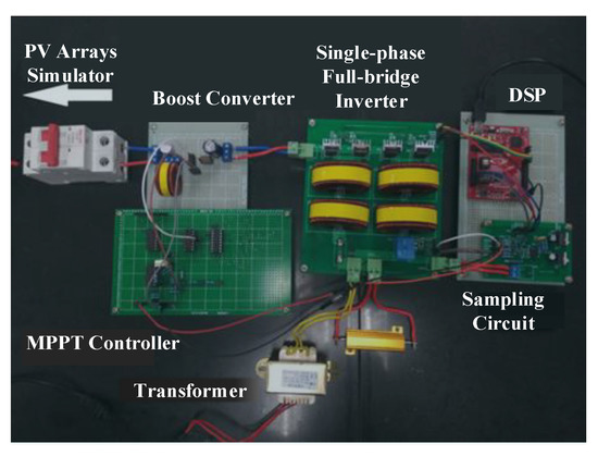
Figure 9.
Experimental setup.
The PV analog power supply uses the Chroma programmable dc current supply 62150H- 1000S. The input capacitor Cin is Panasonic’s 25SEPF330M. The diode VD is General Semiconductor’s FES8JT. The drive power supply uses the IR2101 chip. In the control circuit of the dc-dc converter, the amplifier used a four-channel LM324AD, and the comparator uses a four-channel LM2901. In the dual-loop control of single-phase full-bridge inverter, it is achieved by using the TMS320F28027 micro-processor. The output current is sampled by a WCS2705 Hall sensor. Furthermore, the grid voltage and dc bus voltage sampling circuit are sampled by differential amplifier circuit, and the amplifier adopts TLV2374.
We first investigated what happens when the corresponding circuit of CS is applied. Figure 10 gives a description of the experimental waveform and FFT analysis results of udc in CS under the two sets of MPPT parameters. When Kp1 = 0.11 and Ti1 = 0.01 shown in Figure 10a, the udc waveform approximates a complete sine wave. And the peak voltage appears only at the fundamental frequency multipliers of 100 Hz and 200 Hz in the FFT spectrum, therefore, the system is in a stable state. When Kp1 = 0.11 and Ti1 = 0.00068, udc has a certain degree of distortion, and its FFT spectrum shows a peak at 450 Hz in Figure 10b. The system shows an unstable oscillation phenomenon.
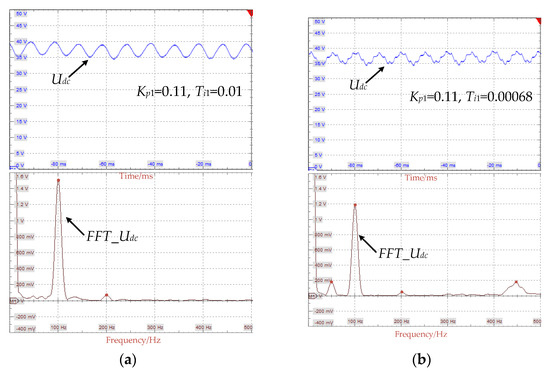
Figure 10.
Experimental waveform and FFT analysis results of dc bus voltage udc in CS at (a) [Kp1, Ti1] = [0.11, 0.01]; (b) [Kp1, Ti1] = [0.11, 0.00068].
Next, we try to find a similar performance when the Boost converter is worked alone. Figure 11 illustrates the experimental waveform and FFT analysis of upv in SS from the three sets of MPPT control parameters. When Kp1 = 0.11 and Ti1 = 0.01, upv is basically going to keep the voltage at the maximum power point as shown in Figure 11a. When Kp1 = 0.11 and Ti1 = 0.001, upv exhibits a small oscillation. It can be seen from the FFT diagram of Figure 11b that there is an intermediate frequency oscillation about at 530 Hz. When Kp1 = 0.11 and Ti1 = 0.00068, as shown in Figure 11c, the voltage waveform appears more severely distorted for the oscillation amplitude is increased, and a medium-frequency oscillation nearly appears at 420 Hz. Thus, the system becomes unstable.
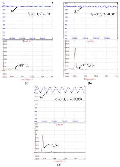
Figure 11.
Experimental waveform and FFT analysis results of PV array output voltage upv in SS at (a) [Kp1, Ti1] = [0.11, 0.01]; (b) [Kp1, Ti1] = [0.11, 0.001]; (c) [Kp1, Ti1] = [0.11, 0.00068].
Comparing Figure 10 with Figure 11, we obtained the same stability analysis results when the two structures operate in the same MPPT parameters. It is in accordance with the description of stable boundary from Section 4. Additionally, the oscillation frequencies of Figure 11b,c are substantially the same as those of the theoretical values obtained in Table 2. Consequently, the consequences obtained in the earlier sections are validated in the experiments.
6. Conclusions
For two-stage PV system, this research uses SS instead of CS to simplify the parameter design of the front-stage dc-dc converter, which can avoid the influence of the parameter coupling in CS. To linearize the nonlinear characteristics of the output current and output voltage in PV array, the average model of SS is established by small-signal analysis method, and, further, the eigenvalue matrix is obtained. Relative eigenvalue sensitivity measure indicates that Kp1, Ti1, Cin, and Lb of the dc-dc converter can exert the equally major effect on one oscillating mode and one attenuating mode in SS and CS. It is also verified through damping ratio and root-locus analysis. By curving the stability boundaries of MPPT controller parameters Kp1 and Ti1 in the aforementioned two structures, the comparison of the two broken-line shows that they have approximate stability domains, and five sets of MPPT examples analyzed in the two structures have the similar stability, which further validates the feasibility of SS instead of CS to design the front-stage dc-dc converter. Furthermore, the modal participation factor is used to describe the interaction between SS and CS. It shows the mode related to the parameters in dc-dc converter is hardly affected by other parts of two-stage PV system. Finally, two sets of MPPT examples tested in CS and three sets of MPPT examples tested in SS perform show almost identical stability, and it is also in accordance with the analysis above in the oscillation frequency. All of which point toward the conclusion that, in two-stage PV system with dc bus, the simplified structure can be used to replace the cascade structure for parameter design optimization of the dc-dc converter.
Author Contributions
Conceptualization, F.X.; Formal analysis, Z.L.; Investigation, L.H.; Methodology, D.Q. and L.H.; Validation, Z.L.; Writing—original draft, Z.L.; Writing—review & editing, F.X., D.Q., B.Z. and Y.C.
Funding
This research was funded by the Key Program of National Natural Science Foundation of China, grant number 2018YFB0905804, the Team Program of Natural Science Foundation of Guangdong Province, China, grant number 2017B030312001, and the National Natural Science Foundation of China, grant number 51507068.
Conflicts of Interest
The authors declare no conflict of interest.
References
- Kjaer, S.B.; Pedersen, J.K.; Blaabjerg, F. A review of single-phase grid-connected inverters for photovoltaic modules. IEEE Trans. Ind. Appl. 2005, 41, 1292–1306. [Google Scholar] [CrossRef]
- Pandey, A.K.; Tyagi, V.V.; Selvaraj, J.A.L.; Rahim, N.A.; Tyagi, S.K. Recent advances in solar photovoltaic systems for emerging trends and advanced applications. Renew. Sustain. Energy Rev. 2016, 53, 859–884. [Google Scholar] [CrossRef]
- Li, Q.; Wolfs, P. A review of the single phase photovoltaic module integrated converter topologies with three different DC link configurations. IEEE Trans. Power Electron. 2008, 23, 1320–1333. [Google Scholar]
- Darwish, A.; Massoud, A.M.; Holliday, D.; Ahmed, S.; Williams, B.W. Single-stage three-phase differential-mode buck-boost inverters with continuous input current for PV applications. IEEE Trans. Power Electron. 2016, 31, 8218–8236. [Google Scholar] [CrossRef]
- Haroun, R.; Aroudi, A.E.; Cid-Pastor, A.; Garcia, G.; Olalla, C.; Martinez-Salamero, L. Impedance matching in photovoltaic systems using cascaded Boost converters and sliding-mode control. IEEE Trans. Power Electron. 2015, 30, 3185–3199. [Google Scholar] [CrossRef]
- Martins, D.C.; Demonti, R. Photovoltaic energy processing for utility connected system. In Proceedings of the 27th Annual Conference of the IEEE Industrial-Electronics-Society, Denver, CO, USA, 29 November–2 December 2001; Volume 1–3. [Google Scholar]
- Prapanavarat, C.; Barnes, M.; Jenkins, N. Investigation of the performance of a photovoltaic AC module. Proc. IEE Gener. Transm. Distrib. 2002, 149, 472–478. [Google Scholar] [CrossRef]
- Al-Hindawi, M.M.; Abusorrah, A.; Al-Turki, Y.; Giaouris, D.; Mandal, K.; Banerjee, S. Nonlinear dynamics and bifurcation analysis of a boost converter for battery charging in photovoltaic applications. Int. J. Bifurc. Chaos 2014, 24, 373–491. [Google Scholar] [CrossRef]
- Zhioua, M.; Aroudi, A.E.; Belghith, S.; Bosque-Moncusí, J.M.; Giral, R.; Al Hosani, K.; Al-Numay, M. Modeling, dynamics, bifurcation behavior and stability analysis of a DC–DC boost converter in photovoltaic systems. Int. J. Bifurc. Chaos 2016, 26, 458–471. [Google Scholar] [CrossRef]
- Huang, M.; Ji, H.; Sun, J.; Wei, L.; Zha, X. Bifurcation based stability analysis of photovoltaic-battery hybrid power system. IEEE J. Emerg. Sel. Top. Power Electron. 2017, 5, 1055–1067. [Google Scholar] [CrossRef]
- Wang, L.; Lin, Y.H. Small-signal stability and transient analysis of an autonomous PV system. In Proceedings of the IEEE/PES Transmission & Distribution Conference & Exposition, Chicago, IL, USA, 21–24 April 2008. [Google Scholar]
- Ge, J.; Du, H.; Zhao, D.; Ma, J.; Qian, M.; Zhu, L. Influences of grid-connected photovoltaic power plants on low frequency oscillation of multi-machine power systems. Autom. Electr. Power Syst. 2016, 40, 63–70. [Google Scholar]
- Gao, B.; Yao, L.; Li, R. Analysis on oscillation modes of large-scale grid-connected PV power plant. Electr. Power Autom. Equip. 2017, 37, 123–130. [Google Scholar]
- Tse, K.K.; Ho, M.T.; Chung, H.S.H.; Hui, S.Y. A novel maximum power point tracker for pv panels using switching frequency modulation. IEEE Trans. Power Electron. 2002, 17, 980–989. [Google Scholar] [CrossRef]
- Koutroulis, E.; Kalaitzakis, K.; Voulgaris, N.C. Development of a microcontroller-based, photovoltaic maximum power point tracking control system. IEEE Trans. Power Electron. 2001, 16, 46–54. [Google Scholar] [CrossRef]
- Sreekanth, T.; Lakshminarasamma, N.; Mishra, M.K. A Single-stage grid-connected high gain buck-boost inverter with maximum power point tracking. IEEE Trans. Energy Convers. 2017, 32, 330–339. [Google Scholar] [CrossRef]
- Saublet, L.M.; Gavagsaz-Ghoachani, R.; Martin, J.P.; Nahid-Mobarakeh, B.; Pierfederici, S. Asymptotic stability analysis of the limit cycle of a cascaded DC–DC converter using sampled discrete-time modeling. IEEE Trans. Ind. Electron. 2016, 63, 2477–2487. [Google Scholar] [CrossRef]
- Zadeh, M.K.; Gavagsaz-Ghoachani, R.; Pierfederici, S.; Nahid-Mobarakeh, B.; Pierfederici, S. Stability analysis and dynamic performance evaluation of a power electronics-based DC distribution system with active stabilizer. IEEE J. Emerg. Sel. Top. Power Electron. 2016, 4, 93–102. [Google Scholar] [CrossRef]
- Xie, F.; Zhang, B.; Qiu, D.; Jiang, Y. Non-linear dynamic behaviours of DC cascaded converters system with multi-load converters. IET Power Electron. 2016, 9, 1093–1102. [Google Scholar] [CrossRef]
- Huang, L.; Qiu, D.; Xie, F.; Chen, Y.; Zhang, B. Modeling and stability analysis of a single-phase two-stage grid-connected photovoltaic system. Energies 2017, 10, 2176. [Google Scholar] [CrossRef]
- Aroudi, A.E.; Giaouris, D.; Mandal, K.; Banerjee, S.; Al-Hindawi, M.; Abusorrah, A.; Al-Turki, Y. Complex nonlinear phenomena and stability analysis of interconnected power converters used in distributed power systems. IET Power Electron. 2016, 9, 855–863. [Google Scholar] [CrossRef]
- Figueres, E.; Garcera, G.; Sandia, J.; Gonzalez-Espin, F.; Rubio, J.C. Sensitivity study of the dynamics of three-phase photovoltaic inverters with an LCL grid filter. IEEE Trans. Ind. Electron. 2009, 56, 706–717. [Google Scholar] [CrossRef]
- Moradi-Shahrbabak, Z.; Tabesh, A. Effects of front-end converter and DC-link of a utility-scale PV energy system on dynamic stability of a power system. IEEE Trans. Ind. Electron. 2018, 65, 403–411. [Google Scholar] [CrossRef]
- Yang, S.; Lei, Q.; Peng, F.; Qian, Z. A robust control scheme for grid-connected voltage-source inverters. IEEE Trans. Ind. Electron. 2011, 58, 202–212. [Google Scholar] [CrossRef]
- Ouyang, Y.; Zou, Y. Static stability analysis of outer-loop control in grid-connected inverters under weak grid condition. In Proceedings of the International Conference on Power System Technology (POWERCON), Guangzhou, China, 6–8 November 2018. [Google Scholar]
- Viinamäki, J.; Jokipii, J.; Messo, T.; Suntio, T.; Sitbon, M.; Kuperman, A. Comprehensive dynamic analysis of photovoltaic generator interfacing DC–DC boost power stage. IET Renew. Power Gener. 2015, 9, 306–314. [Google Scholar] [CrossRef]
- Khouzam, K.; Cuong, L.; Chen, K.K.; Poo, Y.N. Simulation and real-time modelling of space photovoltaic systems. In Proceedings of the IEEE 1st World Conference on Photovoltaic Energy Conversion, Waikoloa, HI, USA, 5–9 December 1994; Volume 2, pp. 2038–2041. [Google Scholar]
- Hung, M.F.; Tseng, K.H. Study on the corresponding relationship between dynamics system and system structural configurations-Develop a universal analysis method for eliminating the RHP-zeros of system. IEEE Trans. Ind. Electron. 2018, 65, 5774–5784. [Google Scholar] [CrossRef]
- Gao, F.; Li, D.; Loh, P.C.; Tang, Y.; Wang, P. Indirect dc-link voltage control of two-stage single-phase PV inverter. In Proceedings of the IEEE Energy Conversion Congress and Exposition, San Jose, CA, USA, 20–24 September 2009; pp. 1166–1172. [Google Scholar]
- Yazdani, A.; Dash, P.P. A control methodology and characterization of dynamics for a photovoltaic (PV) system interfaced with a distribution network. IEEE Trans. Power Deliv. 2009, 24, 1538–1551. [Google Scholar] [CrossRef]
© 2019 by the authors. Licensee MDPI, Basel, Switzerland. This article is an open access article distributed under the terms and conditions of the Creative Commons Attribution (CC BY) license (http://creativecommons.org/licenses/by/4.0/).