Estimation of Static Young’s Modulus for Sandstone Formation Using Artificial Neural Networks

Abstract

In this study, we used artificial neural networks (ANN) to estimate static Young’s modulus (E_static) for sandstone formation from conventional well logs. ANN design parameters were optimized using the self-adaptive differential evolution optimization algorithm. The ANN model was trained to predict E_static from conventional well logs of the bulk density, compressional time, and shear time. The ANN model was trained on 409 data points from one well. The extracted weights and biases of the optimized ANN model was used to develop an empirical relationship for E_static estimation based on well logs. This empirical correlation was tested on 183 unseen data points from the same training well and validated using data from three different wells. The optimized ANN model estimated E_static for the training dataset with a very low average absolute percentage error (AAPE) of 0.98%, a very high correlation coefficient (R) of 0.999 and a coefficient of determination (R²) of 0.9978. The developed ANN-based correlation estimated E_static for the testing dataset with a very high accuracy as indicated by the low AAPE of 1.46% and a very high R and R² of 0.998 and 0.9951, respectively. In addition, the visual comparison of the core-tested and predicted E_static of the validation dataset confirmed the high accuracy of the developed ANN-based empirical correlation. The ANN-based correlation overperformed four of the previously developed E_static correlations in estimating E_static for the validation data, E_static for the validation data was predicted with an AAPE of 3.8% by using the ANN-based correlation compared to AAPE’s of more than 36.0% for the previously developed correlations.

1. Introduction

Young’s modulus is a measure of the sample stiffness against being subjected to a uniaxial load [1]. Static Young’s modulus (E_static) is an essential parameter required to develop the geomechanical earth model [2] which is required for fracture mapping and designing [3]. A complete description of the in-situ stresses which requires assessment of different petrophysical and mechanical parameters is also needed during the drilling operations to ensure wellbore stability [4]. Several previous studies confirmed the impact of the E_static on both fracture design and wellbore stability [1,5].

Lithology is one of the main factors affecting the E_static. According to Howard and Fast [6] and Fjaer et al. [1], E_static for shale ranges from 0.1–1.0 MPsi; for sandstone it is between 2 and 10 MPsi; and for limestone it is between 8 and 12 MPsi [6]. These ranges confirm the very large variation in E_static in different formations, as well as the wide range for same lithology type. These facts indicate the necessity to estimate E_static along the different sections of the drilled well.

Currently, two methods are available for assessing the rocks elastic parameters, these are, namely, (1) laboratory measurements, and (2) through applying empirical correlations. The elastic properties of a rock sample could be measured in the laboratory using either dynamic or static method. The dynamic method involves estimating the modulus from measurements of density, compressional and shear waves velocities while the static method directly measures the deformation in the rock caused by subjecting a sample to uniaxial or triaxial load [7]. In oil and gas fields, the shear and compressional wave velocities measured by the wireline logging [8]. The determined acoustic velocities are then used to calculate the dynamic Young’s modulus (E_dynamic), Equation (1):

$${\mathrm{E}}_{\mathrm{dynamic}}=\frac{\rho {\mathrm{V}}_{\mathrm{S}}{}^2\left(3{\mathrm{V}}_{\mathrm{P}}{}^2-4{\mathrm{V}}_{\mathrm{S}}{}^2\right)}{{\mathrm{V}}_{\mathrm{P}}{}^2-{\mathrm{V}}_{\mathrm{S}}{}^2}$$

(1)

where ρ represents the bulk formation density in g/cm³, V_S and V_P denote the shear and compressional wave’s velocities in km/s, and E_dynamic is the dynamic Young’s modulus in GPa.

For the same rock, usually the laboratory-measured E_dynamic is significantly greater than E_static [9,10,11]. E_dynamic could be 1.5–3 times greater than E_static [12,13], and in some cases E_dynamic could be up to ten times larger than E_static [14,15,16]. The difference is attributed to the strain amplitude between the two testing techniques, and it decreases with the increase in the strength of the rock [17].

The reservoir in situ stress-strain conditions are truly represented by the static elastic parameters [18], determination of these parameters requires retrieval of real core samples along the reservoir section which is a costly and time-consuming process [13,19]. To minimize the high cost of retrieving the core samples and performing laboratory tests; usually few cores samples are collected from the targeted (reservoir) interval, the laboratory evaluated properties of these core samples are used to develop empirical correlations based on the well log data, to evaluate the required core-derived properties. Dynamic elastic modulus could then be calibrated using these log-based correlations to predict the static modulus throughout the reservoir depths [3]. The applicability of log-derived correlations will be restricted to the formations used to develop these correlations, thus, because of the complexity of the heterogeneous formations, the log-derived correlations will not be able to capture the trend of the static parameters changes. To overcome this limitation different empirical correlations were developed to estimate E_static from the E_dynamic, every correlation is restricted for a specific formation type.

Eissa and Kazi [20] developed a generalized empirical equation to predict the E_static as a function of both Edynamic and formation density. The authors developed this correlation (Equation (2)) based on the regression analysis of 76 tests, with data collected from different sources, and they found that considering the formation density improved the predictability of the E_static considerably:

$${\log }_{10}{\mathrm{E}}_{\mathrm{static}}=0.02+0.77{\log }_{10}\left({\mathsf{\gamma }\mathrm{E}}_{\mathrm{dynamic}}\right)$$

(2)

where E_static and E_dynamic are in Gpa, and γ is the formation density in g/cm³.

Canady [21] developed another generalized empirical correlation (Equation (3)) which could also be used effectively to estimate the E_static for any rock type. This correlation enabled prediction of the E_static where only E_dynamic is known, the results of the E_static predicted with (Equation (3)) was compared to previously available correlations and it found to be well correlated to these models:

$${\mathrm{E}}_{\mathrm{static}}=\frac{\ln \left({\mathrm{E}}_{\mathrm{dynamic}}+1\right)\times \left({\mathrm{E}}_{\mathrm{dynamic}}-2\right)}{4.5}$$

(3)

where E_static and E_dynamic are in GPa.

Najibi et al [22] developed another simple correlation (Equation (4)) to evaluate the E_static for Sarvak and Asmari limestone based on only the compressional velocity (Vp). This model is very useful when the shear velocity (Vs) is not available:

E_static = 0.169 × V_P^3.24

(4)

where E_static is in Gpa, and Vp is in km/s.

Recently, Fei et al. [23] developed an empirical correlation to predict E_static from E_dynamic especially for sandstone formation. The developed equation (Equation (5)) is based on the triaxial tests conducted on 22 sandstone core samples:

$${\mathrm{E}}_{\mathrm{static}}=\left(0.564{\mathrm{E}}_{\mathrm{dynamic}}\right)-3.4941$$

(5)

E_static and E_dynamic are in GPa.

Mahmoud et al. [24] developed empirical correlations for E_static estimation for different rock types. The developed correlations do not require the knowledge of E_dynamic and they directly evaluated E_static based on the bulk density, shear, and compressional time data.

It is clear from the literature that obtaining the E_static required retrieve cores from specific depth of the well which is costly and time consuming which required to perform the laboratory analysis. In addition, the analysis will be performed for specific well which cannot easily generalized through the entire field while using the developed empirical correlations had their own limitations such as core type, data range and accuracy. The main objective of this study is to develop an ANN model to predict E_static from the well logs using a real field data (592 core and log data points) which were collected from the whole sandstone field. Furthermore, a new empirical correlation will be developed for estimating E_static for sandstone reservoirs; the correlation is developed based on the extracted weights and biases of the optimized ANN model.

2. Uses of Artificial Intelligence in Estimating Rock Mechanical Parameters

The use of artificial intelligence (AI) techniques in many scientific fields, including the petroleum industry, started in the early 1990s. Since then many publications have treated various areas of petroleum engineering, including the prediction of the bubble point pressure, evaluation of drilling mud, interpretation of the well log data, reservoir characterization, recovery factor estimation, optimization of rate of penetration, and many more.

Recent publications (2016–2018) reported several studies that used AI in estimating rock mechanical parameters. These studies used various AI techniques to: predict failure parameter for carbonates [25]; compare ANN, ANFIS, and SVM in predicting static Poisson’s ratio [26]; develop empirical correlation for static Young’s modulus [27]; develop an ANN-based correlation to predict sonic transit time [28]; estimation of the unconfined compressive strength (UCS) based on the ANN [29]; and use ANN in estimating Young’s modulus, Poisson’s ratio, and UCS from log data [30].

3. Methodology

An artificial neural network (ANN) is an artificial intelligence technique developed to enable estimation, classification, identification, decision making by a machine program in various conditions or situations. Different ANN structures are currently available; the simplest ANN structure is called the multi-layered perceptron (MLP) which is used in this study. The MLP consists of a single input layer, one or several hidden layers (mid-layers) and one output layer.

The performance of the ANN depends on many design parameters, such as the training/testing dataset ratio, number of the hidden (training) layers, the number of neurons in each training layer, and the training and transferring functions. The optimization of different combinations of these design parameters requires a long computational time.

Differential evolution (DE) is an accurate, reliable, fast, and robust optimization technique, which has been used to solve effectively different numerical optimization problems. The main limitation for the DE is the need to set the values of the DE control parameters which is problem-dependent, thus, parameter tuning is time-consuming. Omran et al. [31] developed the self-adaptive differential evolution (SaDE) algorithm, which does not require parameter tuning.

In this study, the SaDE optimization algorithm will be used to speed up the optimization process to select the different design parameters of the ANN model to predict E_static. A new empirical correlation for estimating E_static for sandstone reservoirs will be developed based on the extracted weights and biases of the optimized ANN model.

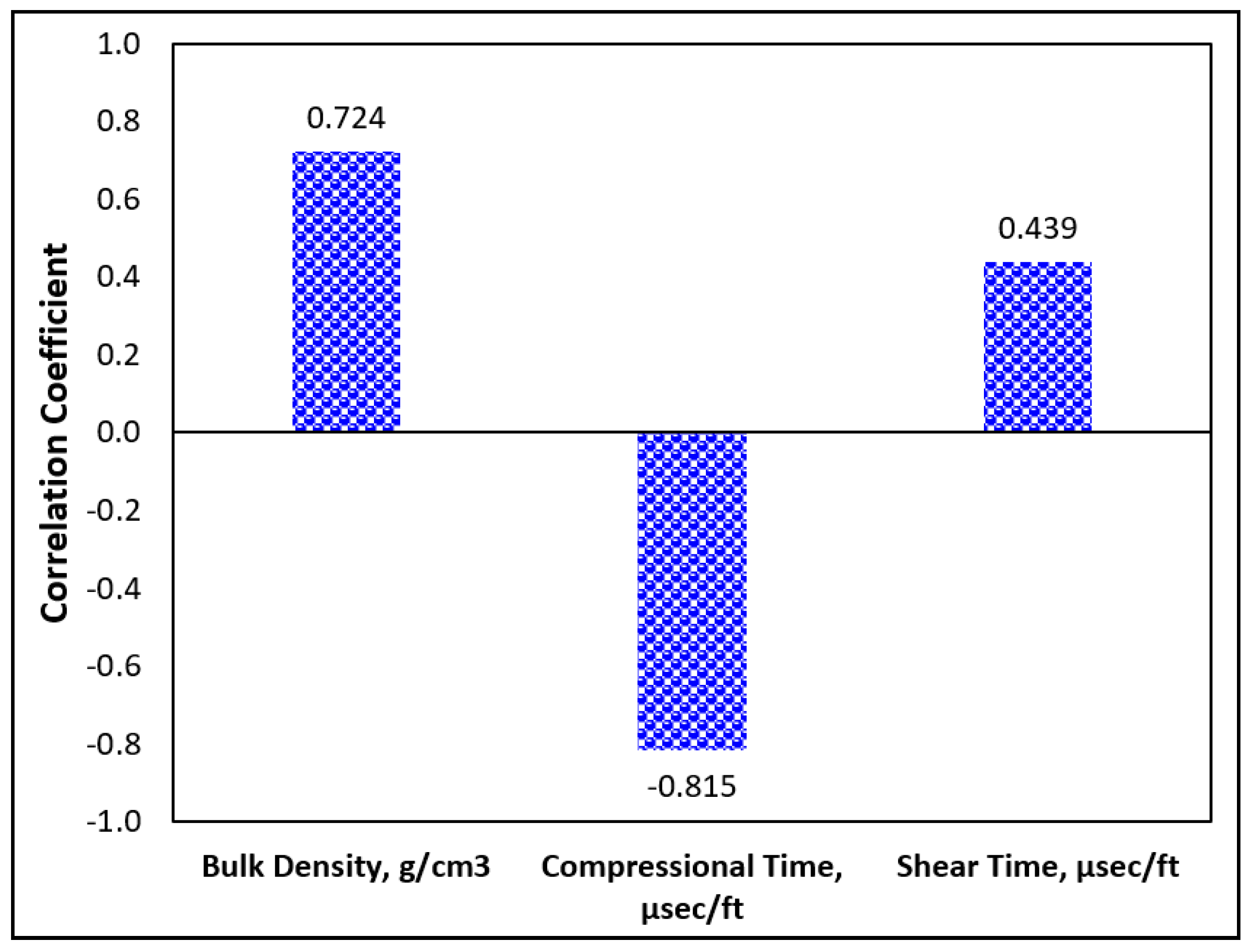
3.1. Data Preparation

In this study, the ANN model was trained using well log data of bulk density, compressional time, and shear time as inputs to predict the core-derived E_static as an output. The input well log data has been selected based on their correlation coefficient with E_static, the importance of the input parameters considered in this study in estimating E_static is reported by several previous studies. Eissa and Kazi [20] confirmed the ability of improving E_static prediction by incorporating the formation density, and the necessity of E_dynamic, which is dependent on the compressional and shear transit times as reported by several previous studies [21,22,23,24].

Data collected in this study are from four wells: 598 data points from Well-A; 34 data points from Well-B; six data points from Well-C; and 11 data points from Well-D. The majority of the data belongs to Well-A, therefore, it will be used to build and test the ANN model which will then be used to develop an ANN-based correlation. The rest of the unseen data which was collected from Well -B, Well-C, and Well-D will be used to validate the developed ANN-based correlation. All the study data are collected from sandstone formations in the Middle East.

Data preparation and preprocessing are the most important steps to ensure a highly accurate prediction of the objective property using any of the AI techniques [32]. As stated earlier the input variables are log-derived, which will be used to predict a core-derived output. Thus, the first step in this study is to perform a depth matching between the core-derived E_static and the log data, gamma ray log was considered to perform the data matching. Then, statistical analysis was performed on the input and output parameters to remove data outliers. For the purpose of outlier removal, all parameter values without a range of ±3.0 standard deviation are considered an outlier and not considered to develop the ANN model. Six data points (outliers) from Well-A were removed in this process.

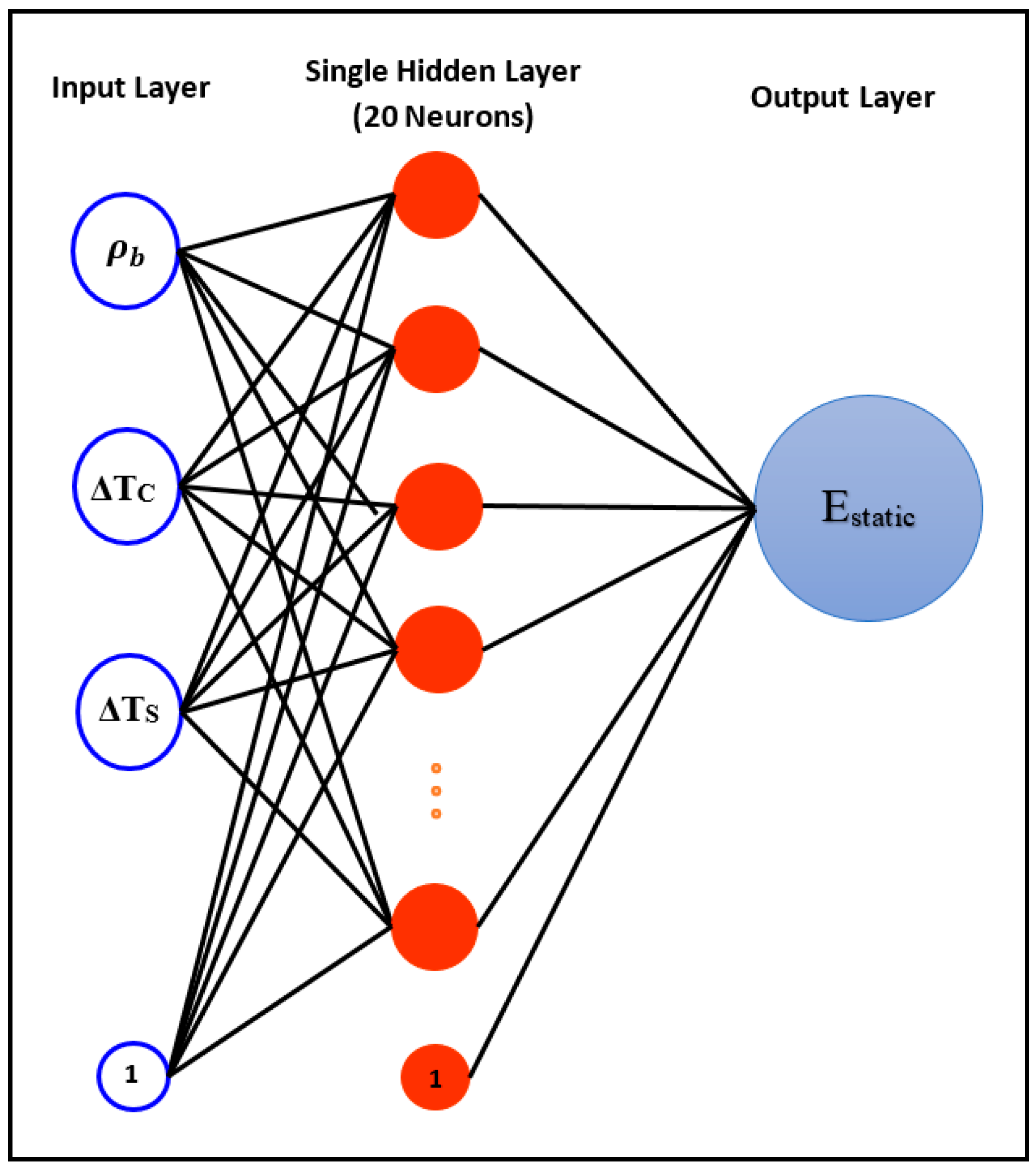
3.2. Training the ANN Model

The 592 data points of Well-A, log data, and their corresponding core-derived E_static were considered as valid data to build the ANN model. Sixty-nine percent (409 data points) of Well-A data, were randomly selected to train the ANN model.

Table 1. Statistics of the training dataset.

Statistical Parameter	ρb, g/cm3	ΔTC, μsec/ft	ΔTS, μsec/ft	Estatic, Gpa
Minimum	2.312	44.3	73.2	7.5
Maximum	2.968	77.8	136.1	92.8
Range	0.656	33.4	62.9	85.3
Standard Deviation	0.106	4.69	8.39	13.93
Sample Variance	0.011	22.0	70.3	194.0
Kurtosis	0.569	4.262	1.673	0.167
Skewness	0.011	1.569	0.564	0.186

summarizes the statistical analysis of the training dataset. The analysis shows that the bulk density (ρ_b) for the input dataset ranges from 2.312–2.968 g/cm³; the compressional time (ΔT_C) ranges between 44.3 and 77.8 μsec/ft; the shear time (ΔT_S) is between 73.2 and 136.1 μsec/ft; and E_static ranges from 7.5–92.8 GPa.

The relative importance of the input parameters is shown in Figure 1. The bulk density and compressional time are strong functions on E_static with correlation coefficients of 0.724 and −0.815, respectively, while the E_static dependence on the shear time is moderate with a correlation coefficient of 0.439.

Design parameters of the ANN model were optimized using the SaDE algorithm, the best combination of design parameters is the one that enables prediction of the E_static with the lowest average absolute percentage error (AAPE), as well as highest correlation coefficient (R) and coefficient of determination (R²). During the optimization process, we evaluated the performance of different training functions such as Levenberg–Marquardt backpropagation (trainlm), gradient descent with momentum backpropagation (traingdm), Gradient descent with adaptive learning rate backpropagation (traingda), Bayesian regularization backpropagation (trainbr), and conjugate gradient (traincgf); different transfer functions such as tan-sigmoid (tansig), log-sigmoid (logsig), and pure line (purelin); number of hidden layers from 1–3; and the number of neurons per each hidden layer from 5 to 30 on estimating the E_static.

The SaDE algorithm was applied using MATLAB software developed by MathWorks (Natick, Massachusetts, U.S.A.) to select the optimum combinations of the ANN design parameters. Based on the optimization process, the combination of the parameters summarized in

Table 2. Combination of the design parameters.

Parameter	Value
Learning function	trainbr
Transfer function	logsig
Number of hidden layers	1
Number of neurons	20

was found to optimize the ANN performance for E_static prediction. As listed in Table 2, trainbr is the best training function that optimizes the E_static predictability of the ANN model. trainbr is a network training function that updates the weight and bias values of for the ANN model based on Levenberg–Marquardt optimization, and it determines the correct output variable after minimizing a combination of weights and squared errors in a process called Bayesian regularization [33]. logsig is the optimum transfer function. The use of a single hidden (training) function (i.e., a single layer) with 20 neurons also optimized predictability of the ANN model for E_static. Figure 2 shows the structure of the suggested ANN model for E_static prediction.

3.3. Evaluation and Validation of the Developed ANN-Based Empirical Correlation

The remaining 31% of the Well-A dataset, which comprises 183 data points, are considered for evaluating the developed ANN-based empirical correlation. Model validation is important step that is preferably performed on unseen data. The three wells (Well-B: 38 data points, Well-C: six data points, and Well-D: 11 data points) are used in model validation. All testing and validation data are within the range of the training data which used to develop the model to ensure high accuracy in predicting E_static. The ability of the developed ANN-based empirical correlation in evaluating the E_static for the validation data collected from Well-B will be compared with four of the available correlations, namely, Eissa and Kazi [20], Canady [21], Najibi et al. [22], and Fei et al. [23] correlations are presented earlier by Equations (2)–(5).

3.4. Evaluation Criterion

The predictive power of the developed ANN-based empirical correlation in estimating E_static will be evaluated based on the AAPE, R², R, and visualization check.

4. Results and Discussion

4.1. Training the ANN Model

The ANN model was trained using 409 randomly selected data points of bulk density, compressional time, and shear time as inputs, and core-derived E_static as output. The training data were collected from Well-A. The optimization process was conducted using the SaDE algorithm. The optimized design parameters of ANN model are summarized in Table 2. Figure 3 shows the well log data and their depth corresponding core-derived and predicted E_static values for the training dataset. As shown in Figure 3 the ANN model predicted the E_static with very high accuracy where the AAPE is only 0.98% and R equals 0.999. A visual check of the plot confirms the excellent matching between the core-derived and the predicted E_static.

Figure 4 presents the cross-plot of the core-derived and the predicted E_static of the training dataset. The ANN model is highly accurate in estimating the E_static as confirmed by the very high R² of 0.9978.

4.2. Developing the ANN-Based Empirical Correlation

The proposed ANN-based empirical model is given in Equations (6)–(10):

$${\mathrm{E}}_{{\mathrm{s}}_n}={\displaystyle \sum }_{i=1}^N{w}_{2_i}\frac{1}{1+e^{-\left(w_{1_{i,1}}{\rho }_{{\mathrm{b}}_{\mathrm{n}}}+w_{1_{i,2}}\mathsf{\Delta }{T}_{{\mathrm{c}}_{\mathrm{n}}}+w_{1_{i,3}}\mathsf{\Delta }{T}_{{\mathrm{s}}_{\mathrm{n}}}+b_{1_i}\right)}}+b_2$$

(6)

where E_sn is the normalized E_static, N represents the number of neurons in the hidden layer (N = 20 neurons), i is the index of each neuron in hidden layer, w_1i denotes the weight associated with input and hidden layers for each input parameter, b_1i is the bias associated with hidden and input layers, w_2i represents the weight associated with hidden and output layers, b₂ is the bias associated with hidden and output layers (b₂ = −1.0767). All weights and biases associated with the hidden and output layers are summarized in

Table 3. The extracted weight and biases of the hidden layer of the optimized ANN model.

i	w1i,1	w1i,2	w1i,3	b1i	w2i
1	−4.368	20.303	−14.485	−3.638	5.437
2	−0.216	1.507	2.017	4.178	−2.494
3	1.792	−2.322	−21.160	−3.877	−4.132
4	0.269	0.057	−0.949	1.777	6.325
5	1.498	−19.164	3.620	6.726	9.261
6	13.802	12.907	−0.662	2.170	0.640
7	3.466	8.897	1.549	−3.110	4.174
8	−4.369	−0.142	17.692	1.732	5.813
9	−1.604	21.932	−1.059	−9.030	5.608
10	10.803	−12.301	24.520	16.752	9.748
11	14.298	13.932	0.070	0.895	−5.642
12	−49.173	−25.972	−1.332	15.768	9.929
13	−3.062	15.989	−11.554	−3.115	−4.766
14	−18.124	−17.674	0.206	−1.307	−3.944
15	40.409	23.746	0.690	−14.273	−11.118
16	6.280	3.526	−8.930	2.199	−0.945
17	7.010	3.251	−11.579	1.502	1.544
18	19.888	7.137	0.149	−8.787	−1.596
19	−32.100	−16.426	−1.400	11.426	−23.697
20	−3.053	1.125	19.499	2.853	−9.194

.

In Equation (6) the values of ρ_bn, ΔT_cn, and ΔT_sn are the normalized input parameters calculated from Equations (7), (8), and (9) respectively:

$${\rho }_{{\mathrm{b}}_{\mathrm{n}}}=2.994\left({\rho }_{\mathrm{b}}-2.312\right)-1$$

(7)

$$\mathsf{\Delta }{\mathrm{T}}_{{\mathrm{c}}_{\mathrm{n}}}=0.0578\left(\mathsf{\Delta }{T}_{\mathrm{c}}-44.341\right)-1$$

(8)

$$\mathsf{\Delta }{\mathrm{T}}_{{\mathrm{s}}_{\mathrm{n}}}=0.0318\left(\mathsf{\Delta }{T}_s-73.187\right)-1$$

(9)

The computed value of E_sn in Equation (6) is in the normalized form and should be converted to real value by using Equation (10):

$${\mathrm{E}}_{\mathrm{s}}=\frac{{\mathrm{E}}_{{\mathrm{s}}_{\mathrm{n}}}+1}{0.0234}+7.4987$$

(10)

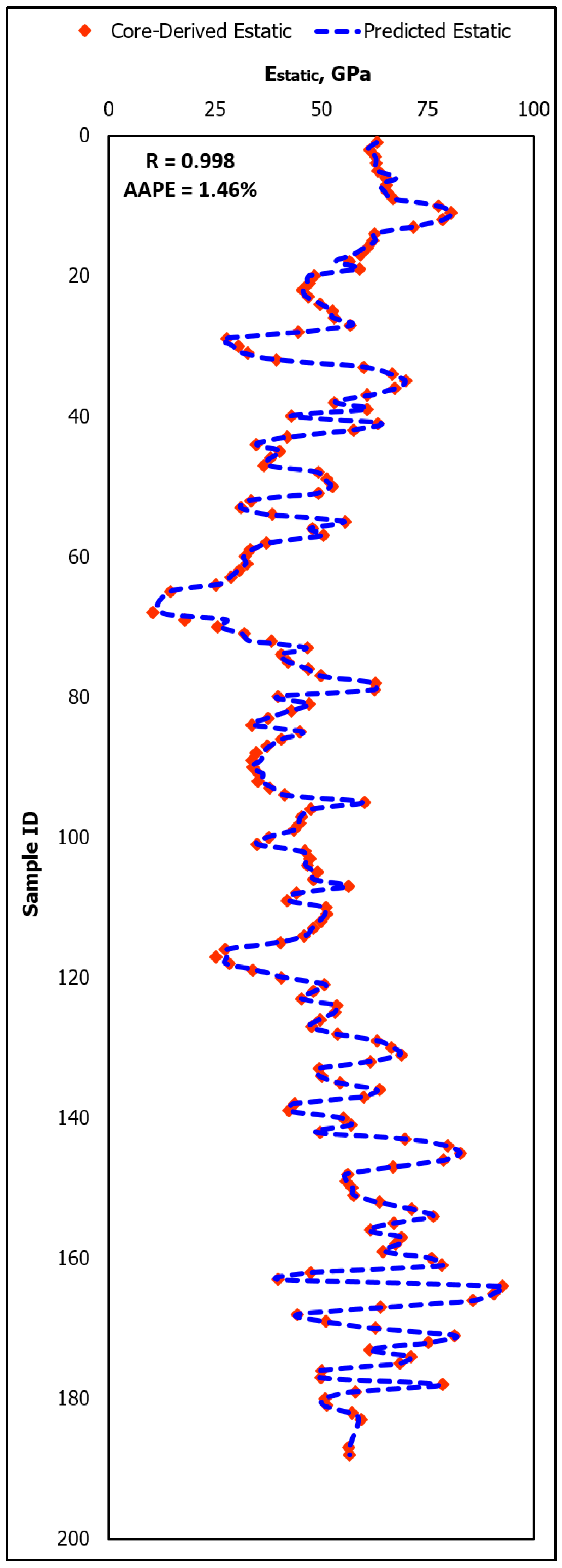
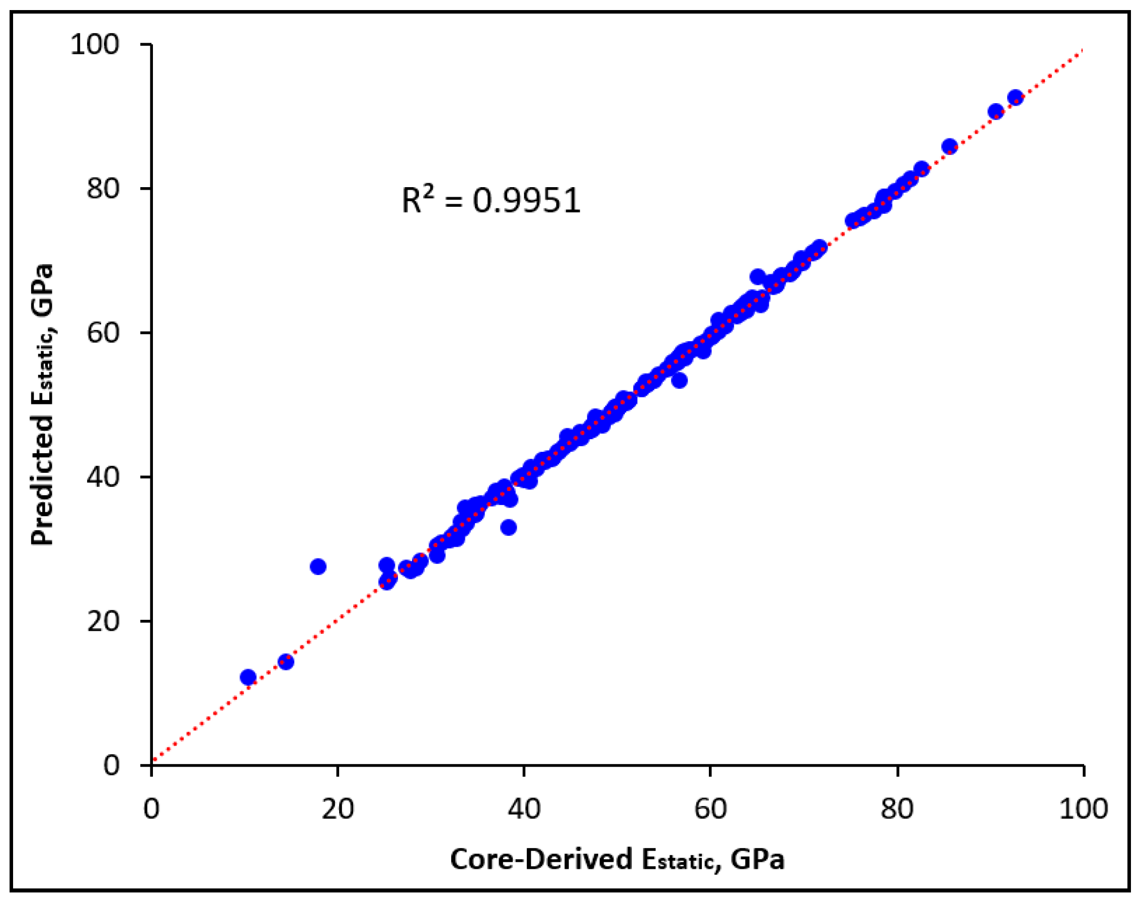
4.3. Testing the Developed ANN-Based Empirical Correlation

The developed ANN-based empirical correlation, Equations (6)–(10), was tested using the 183 unseen, randomly selected, data points from Well-A. Figure 5 compares the core-derived E_static and the estimated E_static. As shown in Figure 5, the ANN-based empirical correlation predicted the E_static for the unseen data with very high accuracy, where the AAPE is only 1.46% and R is 0.998. A visual check of the plot in Figure 5 confirms the excellent matching between the core-derived and predicted E_static.

Figure 6 presents the cross-plot of the core-derived and the predicted E_static of the testing dataset. The ANN-based empirical correlation is highly accurate in estimating the E_static as confirmed by the very high R² of 0.9951.

4.4. Validation of the Developed ANN-Based Empirical Correlation

The developed ANN-based empirical correlation (Equations (6)–(10)) was finally verified using 38 data points from Well-B, six data points from Well-C, and 11 data points from Well-D. Figure 7 compares the core-derived E_static of Well-B and the predicted E_static that developed using ANN-based empirical correlation.

The plot in Figure 7 confirms the highly accurate predictive accuracy of the ANN-based empirical correlation in estimating the E_static; which is validated by the low AAPE of 3.8% and high R of 0.991 in addition to the visual check of the plot. Similarly, the core-derived and the predicted E_static values for Well-C and Well-D were plotted in Figure 7. Due to the limited number of data points in Well-C and Well-D, it was enough to check the predictive accuracy of the ANN-based empirical correlation visually. In all three wells used in validation, the ANN-based empirical correlation was able to provide a continuous profile of the predicted E_static that conforms to the available core-derived values.

Figure 8 presents the cross-plot of the core-derived and the predicted E_static of the 38 data points of Well-B, which are used in validating the ANN-based empirical correlation. This plot affirms the high accuracy of the developed ANN-based empirical correlation in estimating E_static as confirmed by the very high R² of 0.9816.

4.5. Comparing the Developed ANN-Based Empirical Correlation to the Available Correlations

Predictive accuracy of the ANN-based empirical correlation was compared with the accuracy of four available developed correlations. Data collected from Well-B was used for the purpose of this comparison. Figure 9 compares predictive accuracy of the ANN-based correlation with the accuracy of Eissa and Kazi [20], Canady [21], Najibi et al. [22], and Fei et al. [23], correlations in estimating E_static for the validation dataset of Well-B. Eissa and Kazi [20], Canady [21], Najibi et al. [22], and Fei et al. [23] correlations are presented earlier by Equations (2)–(5). As indicated in Figure 9, the ANN-based correlation overperformed all the four correlations in evaluating = E_static with an AAPE of 3.80% compared to an AAPE of 37.2%, 36.3%, 61.7%, and 68.5% for the E_static values predicted using Eissa and Kazi [20], Canady [21], Najibi et al. [22], and Fei et al. [23]. These results confirm the high accuracy of the developed ANN-based empirical correlation for E_static estimation.

5. Conclusions

In this study, self-adaptive differential evolution (SaDE) was employed to optimize the ANN design parameters to predict the static Young’s modulus (E_static) for sandstone formations using well log data of the bulk density, compressional time, and shear time. The ANN model was trained and tested using real field measurements of 592 data points. Based on the results of this study, the following points are concluded:

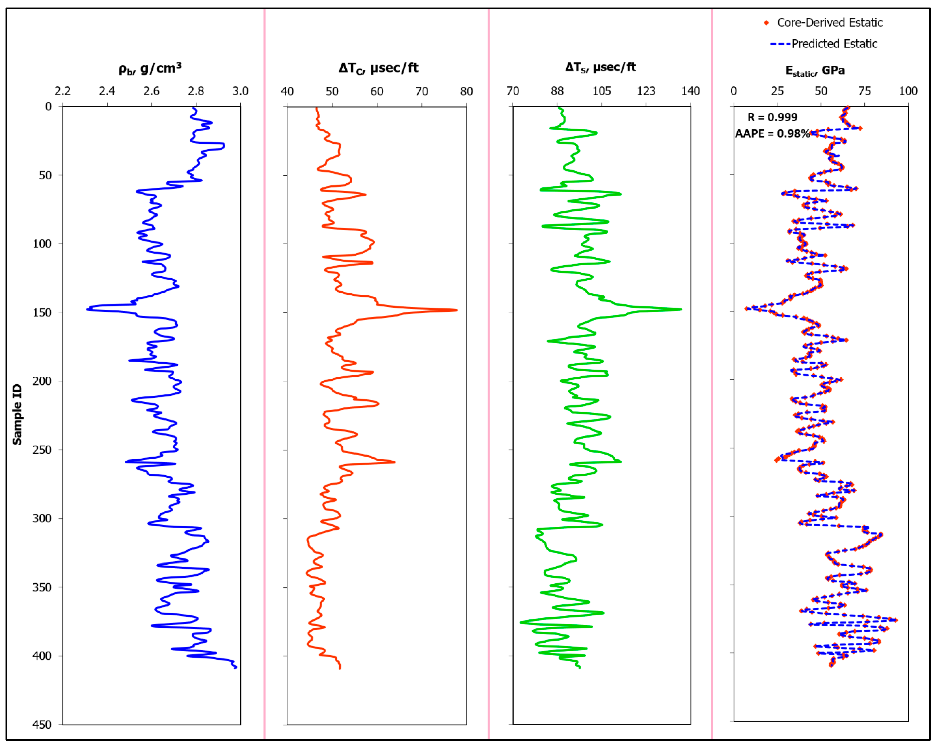
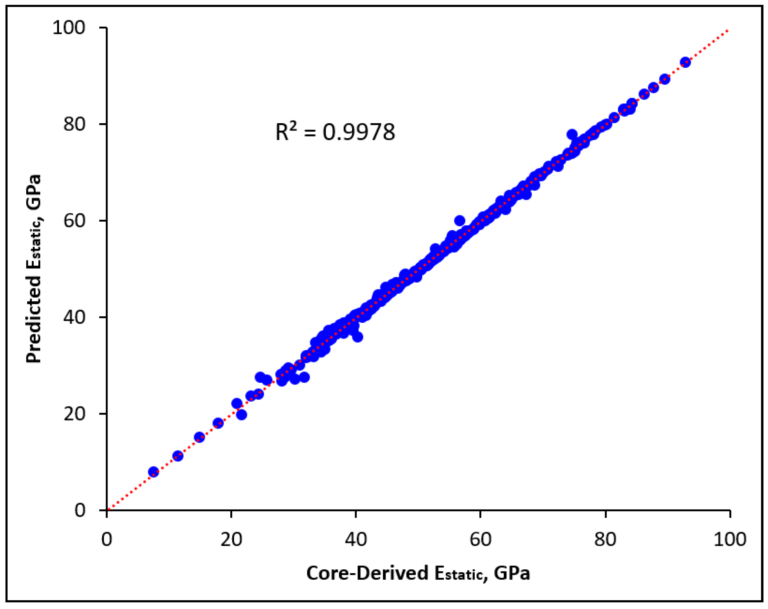
• The developed ANN model was capable of estimating E_static for the training dataset with very high accuracy, as indicated by the low AAPE of 0.98%, very high R of 0.999, and R² of 0.9978. The ANN-based empirical correlation was able to predict E_static for the testing dataset (unseen) accurately; the E_static values of the testing dataset were estimated with AAPE, R, and R² values of 1.46%, 0.998, and 0.9951, respectively.
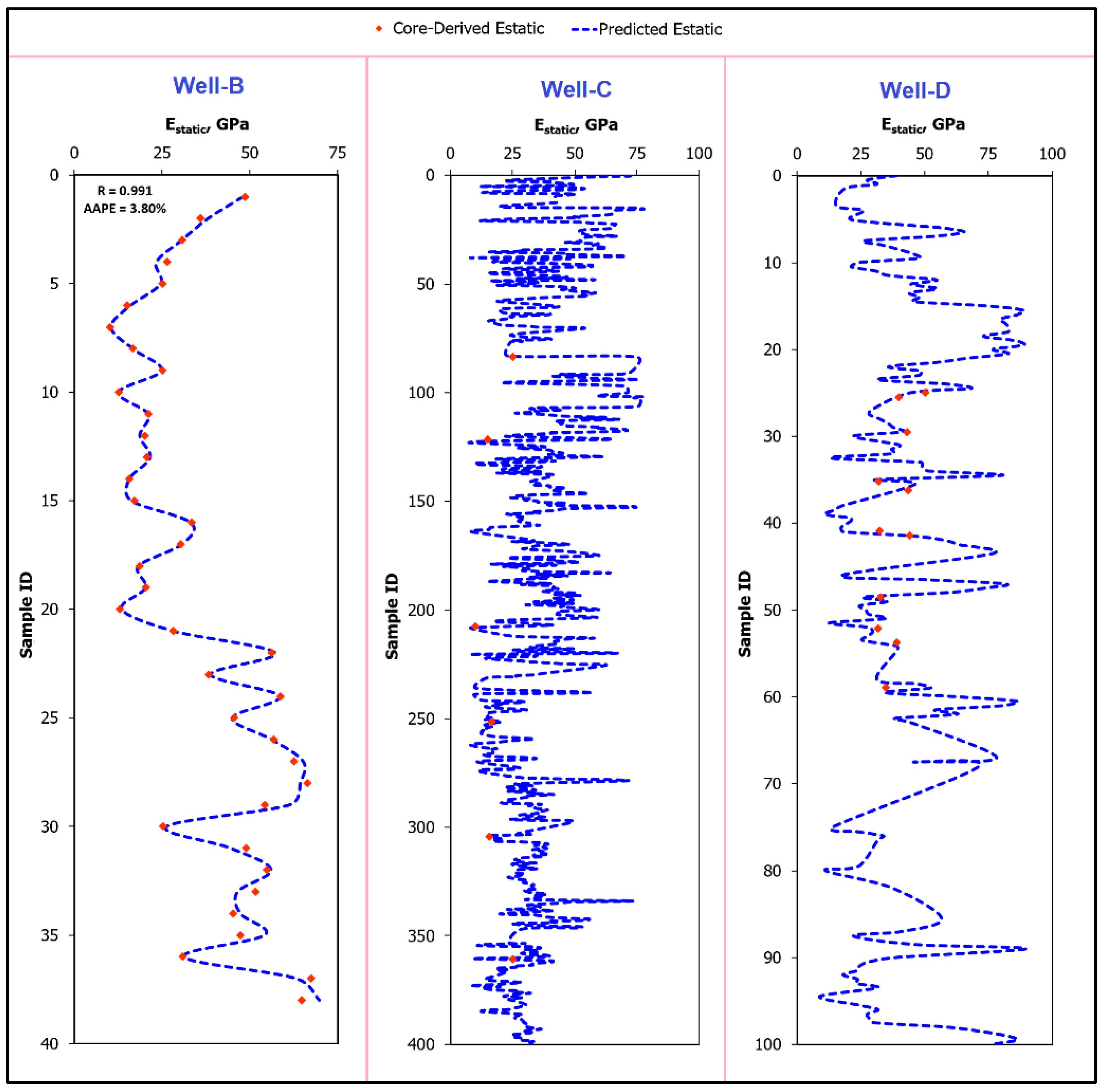
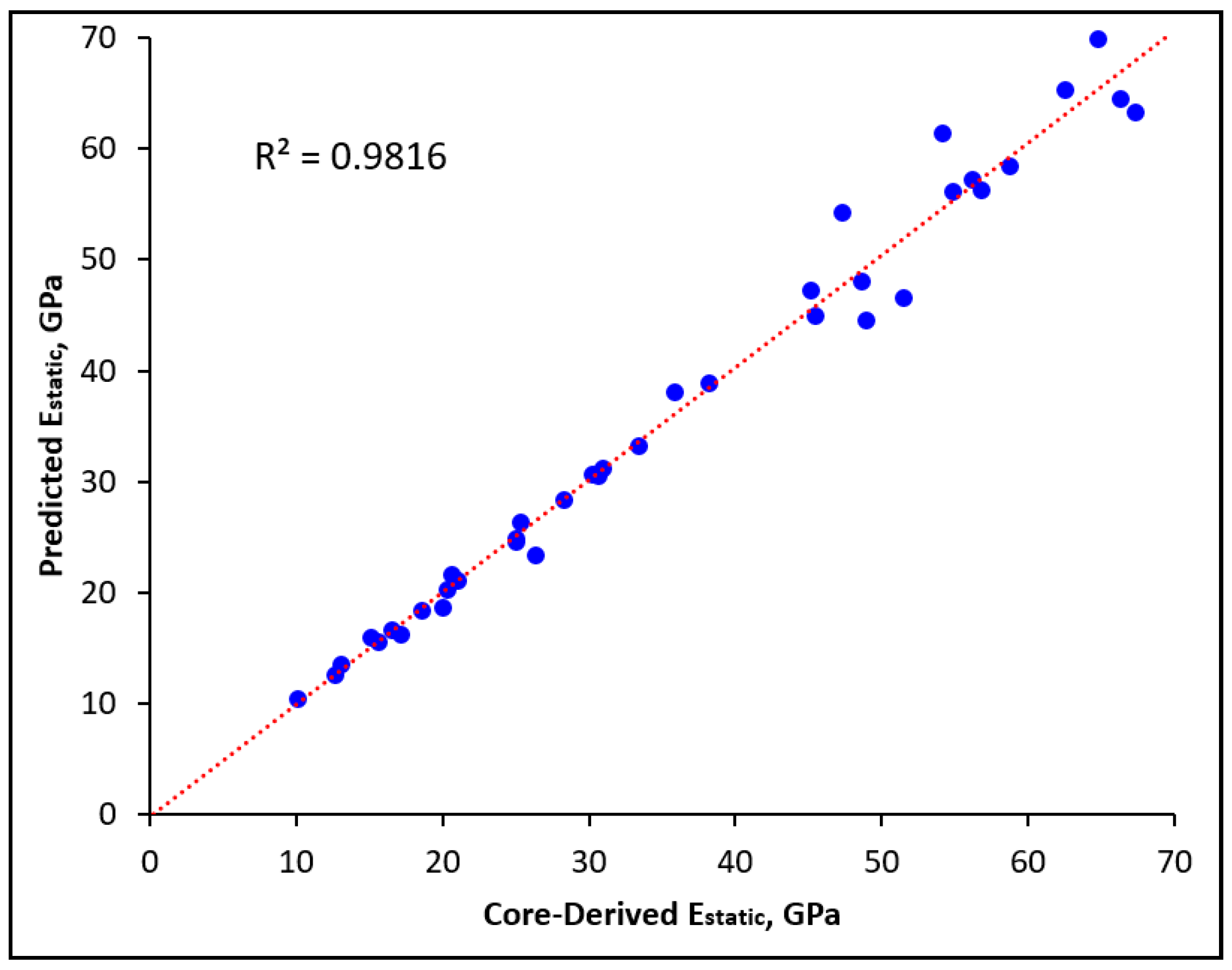
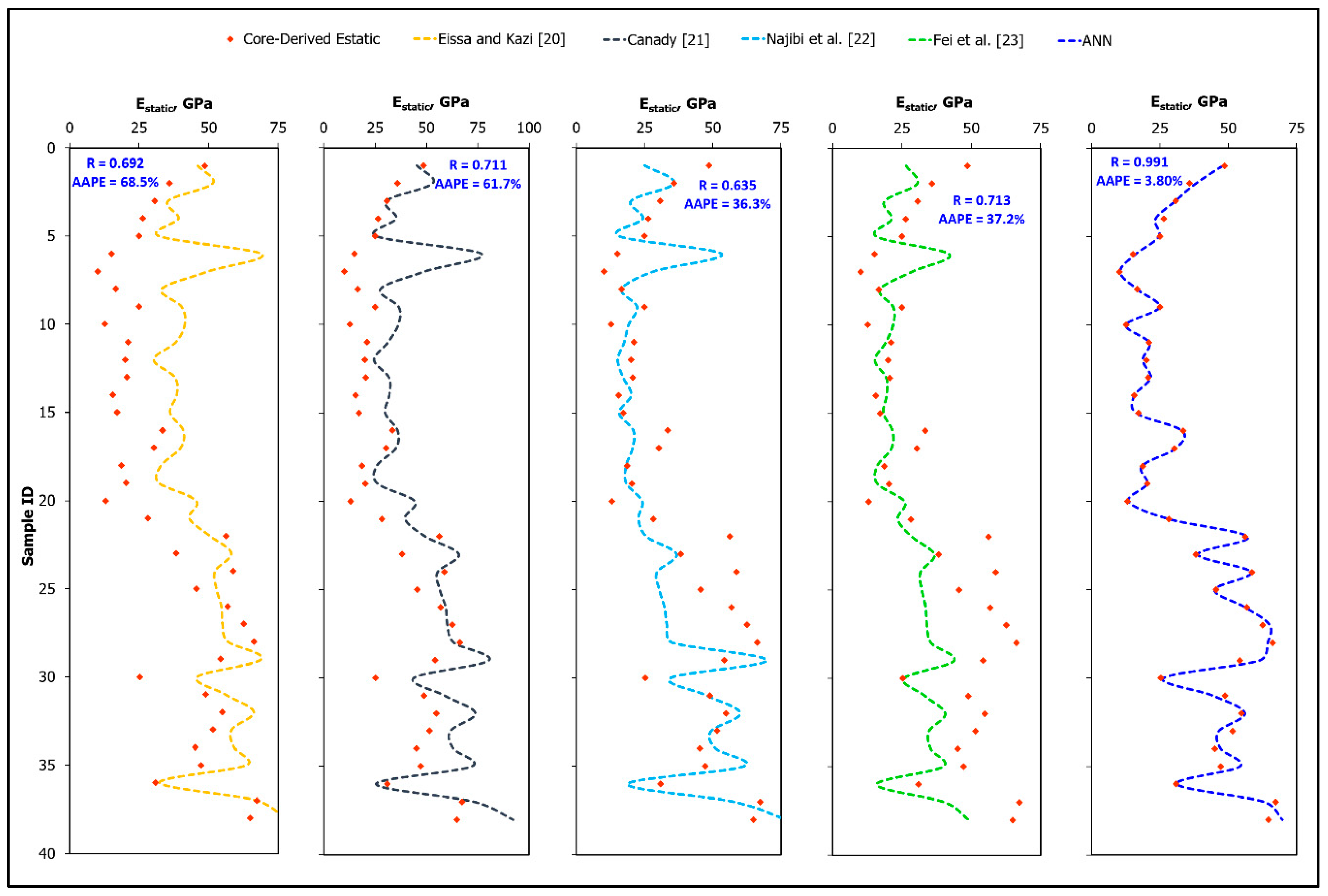
• The developed empirical correlation was validated using a dataset composed of unseen 55 data points of three wells. Validating the developed correlation using the dataset of Well-B (38 points) revealed a highly accurate prediction of the developed correlation where AAPE, R and R² valueswere 3.8, 0.991 and 0.9816 respectively.
• The ANN-based empirical correlation is useful in predicting continuous profile of static Young’s modulus for sandstone formation using conventional log data, bulk density, shear transit time and compressional transit time when there are no available cores.
• Comparing the predictive accuracy of the ANN-based correlation with four of the available empirical equations confirmed the high accuracy of the ANN-based correlation which was able to estimate the E_static for the validation data of Well-B with an AAPE of 3.8% compared with an AAPE of more than 36.0% for all available correlations.

References

1. Fjaer, E.; Horsrud, H.P.; Raaen, A.M.; Risnes, R. Petroleum Related Rock Mechanics; Elsevier B. V.: Amsterdam, The Netherlands, 2008. [Google Scholar]
2. Chang, C.; Zoback, M.D.; Khaksar, A. Empirical relations between rock strength and physical properties in sedimentary rocks. J. Pet. Sci. Eng. 2006, 51, 223–237. [Google Scholar] [CrossRef]
3. Gatens, J.M.; Harrison, C.W.; Lancaster, D.E.; Guldry, F.K. In-situ stress tests and acoustic logs determine mechanical properties and stress profiles in the devonian shales. SPE Form. Eval. 1990, 5, 248–254. [Google Scholar] [CrossRef]
4. Nes, O.M.; Fjaer, E.; Tronvoll, J.; Kristiansen, T.G.; Horsrud, P. Drilling time reduction through an integrated rock mechanics analysis. J. Energy Res. Technol. 2012, 134, 2802:1–2802:7. [Google Scholar] [CrossRef]
5. Meyer, B.R.; Jacot, R.H. Impact of stress-dependent Young’s moduli on hydraulic fracture modeling. In Proceedings of the 38th U.S. Symposium on Rock Mechanics, Washington, DC, USA, 7–10 July 2001. ARMA-01-0297. [Google Scholar]
6. Howard, G.C.; Fast, C.R. Hydraulic Fracturing. In Doherty Memorial Fund of AIME, Society of Petroleum Engineers of AIME; Henry L.: New York, NY, USA, 1970; Monograph Volume 2 of SPE. [Google Scholar]
7. Barree, R.D.; Gilbert, J.V.; Conway, M.W. Stress and rock property profiling for unconventional reservoir stimulation. In Proceedings of the SPE Hydraulic Fracturing Technology Conference, The Woodlands, TX, USA, 19–21 January 2009. SPE-118703-MS. [Google Scholar]
8. Colin, C.; Potter, S.; Darren, F. Formation elastic parameters by deriving S-wave velocity logs. CREWES Res. 1997, 9, 1–10. [Google Scholar]
9. King, M.S. Wave Velocities in Rocks as a Function of Changes in Over burden Pressure and Pore Fluid Saturants. Geophysics 1966, 31, 50–73. [Google Scholar] [CrossRef]
10. Rinehart, J.S.; Fortin, J.-P.; Baugin, P. Propagation Velocity of Longitudinal Waves in Rock. Effect of State of Stress, Stress Level of the Wave, Water Content, Porosity, Temperature Stratification and Texture. In Proceedings of the 4th Symposium on Rock Mechanics, University Park, PA, USA, 30 March–1 April 1961. ARMA-61-119. [Google Scholar]
11. Simmons, G.; Brace, W.I. Comparison of Static and Dynamic Measurements of Compressibility of Rocks. J. Geophys. Res. 1965, 70, 5649–5656. [Google Scholar] [CrossRef]
12. Abdulraheem, A.; Ahmed, M.; Vantala, A.; Parvez, T. Prediction of Rock Mechanical Parameters for Hydrocarbon Reservoirs Using Different Artificial Intelligence Techniques. In Proceedings of the Saudi Arabia Section Technical Symposium, Al-Khobar, Saudi Arabia, 9–11 May 2009. SPE-126094-MS. [Google Scholar]
13. Larsen, I.; Fjær, E.; Renlie, L. Static and Dynamic Poisson’s Ratio of Weak Sandstones. In Proceedings of the 4th North American Rock Mechanics Symposium, Seattle, WA, USA, 31 July–3 August 2000. ARMA-2000-0077. [Google Scholar]
14. Bai, P. Experimental research on rock drillability in the center of junggar basin. Electron. J. Geotech. Eng. 2013, 18, 5065–5074. [Google Scholar]
15. Ca, H.; Xi, L.; Guo, L. Rock mechanics study on the safety and efficient extraction for deep moderately inclined medium-thick orebody. Electron. J. Geotech. Eng. 2015, 20, 11073–11082. [Google Scholar]
16. Li, P.; Liu, X.; Zhong, Z. Mechanical Property Experiment and Damage Statistical Constitutive Model of Hongze Rock Salt in China. Electron. J. Geotech. Eng. 2015, 20, 81–94. [Google Scholar]
17. King, M.S. Static and Dynamic elastic moduli of rocks under pressure. In Proceedings of the 11th U.S. Symposium on Rock Mechanics, Berkeley, CA, USA, 16–19 June 1969. ARMA-69-0329. [Google Scholar]
18. Wang, Z.; Nur, A.A. Dynamic versus static elastic properties of reservoir rocks. J. Seism. Acoust. Veloc. Res. Rocks 2000, 19, 531–539. [Google Scholar]
19. Khaksar, A.; Taylor, P.G.; Fang, Z.; Kayes, T.; Salazar, A.; Rahman, K. Rock strength from core and logs, where we stand and ways to go. In Proceedings of the EUROPEC/EAGE conference and exhibition, Amsterdam, The Netherlands, 8–11 June 2009. SPE-121972-MS. [Google Scholar]
20. Eissa, E.A.; Kazi, A. Relation between static and dynamic Young’s moduli of rocks. Int. J. Rock Mech. Min. Sci. Geomech. Abstr. 1988, 25, 479–482. [Google Scholar] [CrossRef]
21. Canady, W.J. A Method for Full-Range Young’s Modulus Correction. Presented at the North American Unconventional Gas Conference and Exhibition, The Woodlands, TX, USA, 14–16 June 2011. Paper SPE-143604-MS. [Google Scholar] [CrossRef]
22. Najibi, A.R.; Ghafoori, M.; Lashkaripour, G.R.; Asef, M.R. Empirical relations between strength and static and dynamic elastic properties of Asmari and Sarvak limestones, two main oil reservoirs in Iran. J. Pet. Sci. Eng. 2015, 126, 78–82. [Google Scholar] [CrossRef]
23. Fei, W.; Huiyuan, B.; Jun, Y.; Yonghao, Z. Correlation of Dynamic and Static Elastic Parameters of Rock. Electron. J. Geotech. Eng. 2016, 21, 1551–1560. [Google Scholar]
24. Mahmoud, M.A.; Elkatatny, S.A.; Ramadan, E.; Abdulraheem, A. Development of Lithology-Based Static Young’s Modulus Correlations from Log Data Based on Data Clustering Technique. J. Pet. Sci. Eng. 2016, 146, 10–20. [Google Scholar] [CrossRef]
25. Tariq, A.; Elkatatny, S.A.; Mahmoud, M.A.; Zaki, A.; Abdulraheem, A. A New Approach to Predict Failure Parameters of Carbonate Rocks using Artificial Intelligence Tools. In Proceedings of the SPE Kingdom of Saudi Arabia Annual Technical Symposium and Exhibition, Dammam, Saudi Arabia, 24–27 April 2017. SPE-187974-MS. [Google Scholar]
26. Elkatatny, S.M.; Tariq, Z.; Mahmoud, M.A.; Abdulraheem, A.; Abdelwahab, A.Z.; Woldeamanuel, M. An Artificial Intelligent Approach to Predict Static Poisson’s Ratio. In Proceedings of the 51st US Rock Mechanics/Geomechanics Symposium, San Francisco, CA, USA, 25–28 June 2017. ARMA 17-771. [Google Scholar]
27. Tariq, Z.; Elkatatny, S.M.; Mahmoud, M.A.; Abdulazeez, A. A Holistic Approach to Develop New Rigorous Empirical Correlation for Static Young’s Modulus. In Proceedings of the Abu Dhabi International Petroleum Exhibition & Conference, Abu Dhabi, UAE, 7–10 November 2016. SPE-183545-MS. [Google Scholar]
28. Tariq, Z.; Elkatatny, S.M.; Mahmoud, M.A.; Abdulazeez, A. A New Artificial Intelligence Based Empirical Correlation to Predict Sonic Travel Time. In Proceedings of the International Petroleum Technology Conference, Bangkok, Thailand, 14–16 November 2016. IPTC-19005-MS. [Google Scholar]
29. Tariq, Z.; Elkatatny, S.M.; Mahmoud, M.A.; Abdulraheem, A.; Abdelwahab, A.Z.; Woldeamanuel, I.M. Development of New Correlation for Unconfined Compressive Strength for Carbonate Reservoir Using Artificial Intelligence Techniques. In Proceedings of the 51st US Rock Mechanics/Geomechanics Symposium, San Francisco, CA, USA, 25–28 June 2017. ARMA 17-428. [Google Scholar]
30. Tariq, Z.; Elkatatny, S.M.; Mahmoud, M.A.; Abdulraheem, A.; Abdelwahab, A.Z.; Woldeamanuel, M. Estimation of Rock Mechanical Parameters using Artificial Intelligence Tools. In Proceedings of the 51st US Rock Mechanics/Geomechanics Symposium, San Francisco, CA, USA, 25–28 June 2017. ARMA 17-301. [Google Scholar]
31. Omran, M.G.H.; Salman, A.; Engelbrecht, A.P. Self-adaptive Differential Evolution. In Computational Intelligence and Security; Hao, Y., Liu, J., Wang, Y., Cheung, Y.-m., Yin, H., Jiao, L., Ma, J., Jiao, Y.-C., Eds.; CIS 2005. Lecture Notes in Computer Science; Springer: Berlin/Heidelberg, Germany, 2005; Volume 3801. [Google Scholar]
32. Al-Anazi, A.F.; Gates, I.D. A support vector machine algorithm to classify lithofacies and model permeability in heterogeneous reservoirs. Eng. Geol. 2010, 114, 267–277. [Google Scholar] [CrossRef]
33. MathWorks. Available online: https://www.mathworks.com/help/deeplearning/ref/trainbr.html;jsessionid=7cc70c77fdb3f0bb58ed870c69c7 (accessed on 1 April 2019).
Figure 1. The relative importance of the training dataset input parameter.
Energies 12 02125 g001
Figure 2. The designed structure for the ANN model with a single hidden layer and 20 neurons.
Energies 12 02125 g002
Figure 3. From left to right, bulk density, compressional transit time, shear transit time, and their corresponding predicted and core-derived static Young’s modulus values of the training set of Well-A.
Energies 12 02125 g003
Figure 4. Cross-plot of the core-derived and predicted Estatic of the training dataset.
Energies 12 02125 g004
Figure 5. Predicted and core-derived Estatic of the testing data, Well-A.
Energies 12 02125 g005
Figure 6. Cross-plot of the core-derived and predicted Estatic of the testing dataset.
Energies 12 02125 g006
Figure 7. Plot of the predicted and the core-derived Estatic for the validation datasets collected from Well-B, Well-C, and Well-D.
Energies 12 02125 g007
Figure 8. Cross-plot of the core-derived and predicted Estatic of the validation dataset.
Energies 12 02125 g008
Figure 9. Comparison between predictive accuracy of Eissa and Kazi [20], Canady [21], Najibi et al. [22], Fei et al. [23], and ANN-based correlations in estimating Estatic for the validation dataset of Well-B.
Energies 12 02125 g009