Maintenance Strategy Optimization of a Coal-Fired Power Plant Cooling Tower through Generalized Stochastic Petri Nets

Abstract

Determining the ideal size of maintenance staff is a daunting task, especially in the operation of large and complex mechanical systems such as thermal power plants. On the one hand, a significant investment in maintenance is necessary to maintain the availability of the system. On the other hand, it can significantly affect the profit of the plant. Several mathematical modeling techniques have been used in many different ways to predict and improve the availability and reliability of such systems. This work uses a modeling tool called generalized stochastic Petri net (GSPN) in a new way, aiming to determine the effect that the number of maintenance teams has on the availability and performance of a coal-fired power plant cooling tower. The results obtained through the model are confronted with a thermodynamic analysis of the cooling tower that shows the influence of this system’s performance on the efficiency of the power plant. Thus, it is possible to determine the optimal size of the repair team in order to maximize the plant’s performance with the least possible investment in maintenance personnel.

1. Introduction

Electricity generation from coal is one of the most important activities in fossil fuel-based economies across the globe. Today, almost 40% of worldwide electricity production is based on conventional coal-fired power plants [1], as shown in Figure 1. Coal-fired power plants have been in continuous development for a long time with considerable efforts to improve their capacity and thermal efficiency, since an increase in their efficiency can significantly reduce the overall cost of electricity production, as well as reduce the environmental impact generated by the burning of coal [2,3].

The main objective of any electric power generation system is to provide the energy demanded by the market, as well as to comply with the regulatory requirements [4]. In order to do so, it is necessary to ensure its availability, which is the percentage of time in which the system is able to produce electricity at a specified admissible level. Many studies have been developed to predict not only the availability of such power plants, but also the economic performance and the risks associated with their operation [5,6].

The availability of a complex system is strongly associated with its components’ reliability, as well as its maintenance policy. In order to avoid plant’s efficiency degradation, it is vital to develop an adequate maintenance plan, which can also improve the system’s reliability and availability. Several well-established maintenance philosophies have already been implemented in the thermal power plant scenario, such as reliability centered maintenance (RCM) [7,8,9], risk-based maintenance (RBM) [10,11], and condition-based maintenance (CBM) [12,13]. Recent studies also propose the integrated use of some of these philosophies [14,15,16]. Although each of these philosophies proposes the development of maintenance plans under different perspectives, it is important to note that they share the objective of maintaining the integrity and functionality of the system. The main goal of those philosophies is to define an efficient strategy for preventive maintenance planning, mainly focusing on monitoring the condition of components and systems in order to determine a dynamic preventive schedule.

Since maintenance plans can directly improve performance and equipment operational life, several mathematical models can be used to determine the real impact of such plans on the availability and reliability of the system as a whole. A reliability block diagram (RBD), for example, is a technique for system reliability and availability analysis that can be used for this purpose, using information regarding the failure and repair rates of a system’s components [17,18]. A RBD resembles schematic representation of systems where the connections indicate the interdependency and functioning of the systems according to their configuration.

Although a RBD is able to identify the least reliable components in the system, requiring more attention from the maintenance team, this diagrammatic method is unable to represent the behavior of complex systems, especially those that are reconfigured in different operational contexts (such as fault-tolerant systems), and therefore has limited use. In such cases, it is common to use state machines for a more realistic analysis. The Markov chain method is frequently used to represent system reliability and availability, since it is based on the description of all possible system states (based on a combination of failures and operating states of its components), where the transitions between states are associated with failures of components and repair rates. To represent and solve the Markov process, it is necessary to construct the appropriate state space diagram and to insert the relevant transition rates. Sabouhi et al. [18] used this technique to model the reliability and availability of a combined cycle power plant alongside with RBD analysis. Manesh et al. [19] used the Markov method for the determination of availability and reliability of complex cogeneration systems.

In Markov process analysis, there are no basic restrictions on the number of states and transitions used in the model, and the elaboration of the state space diagram, translate the analyst´s knowledge about the system operation. However, the greater the number of components the greater is the difficulty to model the state space. The model can, therefore, become unmanageable for large systems [20].

Dynamic and complex systems, which change their mode of operation or their performance due to failures in their components, can be easily represented by a technique based on Markov chains called Petri net (PN). PN is a modeling method that can represent a system’s structure and dynamic behavior in a formal graph.

This work, which is an evolution of previous publications [21,22], uses a more complex type of PN, namely the generalized stochastic Petri net (GSPN), in a new way, aiming at determining the effect that a predictive maintenance policy can have on the availability, reliability and performance of a coal-fired power plant cooling tower. Since the cooling tower under study is composed of several components that can fail simultaneously, the proposed GSPN model is also able to determine the effect of an expansion on the maintenance team in the system. Despite being a redundant subsystem, the cooling towers may present degradation in their components that can reduce their heat transfer capacity in comparison with design conditions, decreasing plant efficiency. So the maintenance planners should give attention to the cooling towers subsystem aiming at avoiding its degradation.

The results obtained through the model are also confronted with a thermodynamic analysis showing the influence of the cooling tower performance on the overall efficiency of the power plant. As a result, it is possible to determine the optimal size of the repair work force in order to maximize the plant’s performance with the least possible investment in maintenance personnel. The study was carried out using actual operational data gathered in a coal-fired power plant in the northeast of Brazil. The results obtained show that coal savings due to improved efficiency compensate the investment in a better cooling tower maintenance strategy.

2. Generalized Stochastic Petri Nets (GSPN)

The original concept of PNs was developed by Carl Adam Petri back in 1962. Initially, it was developed for modeling and analysis of computer hardware and software, but during the last few years PN has been increasingly used in engineering areas such as automation, communication, chemistry, civil engineering, and reliability systems [23]. The graphical representation of PN employs the following notations: Places (described by circles), Transitions (described by boxes or bars), Arcs (described by arrows that connect Places to Transitions and vice versa), and Tokens (described by a black dot). The tokens located in a place are referred to as the marking of a place; the initial marking represents the initial condition or state of the PN [24].

A basic model of a Petri net is shown in Figure 2. It shows the PN with two places (P₁ and P₂), and between them an immediate transition (t₁). Places can be occupied by one or more tokens [25]. The graphical construction of a PN involves the understanding of how the places, transitions, tokens and arcs interact. The dynamic behavior of a PN is described by a sequence of transition firings. Firing results in moving one token from one place to another place by a transition. Arcs determine the path that tokens take throughout the model. They can either enable or inhibit movement in the model, depending on their use.

A PN can be represented mathematically as a quintuple [26]:

PN = (P, T, Pre, Post, M₀), where:

• P = {P₁, P₂, … P_m} is a finite set of places;
• T = {t₁, t₂, …, t_m} is a finite set of transitions;
• Pre: P × T is the place application;
• Post: P × T is the following place application
• M₀ = {0, 1, 2, 3, …, i_th} is the initial marking of the PN, represents the number of tokens in the i_th place.

The original Petri net did not include the concept of time, i.e., transitions would fire immediately if enabled. However, starting in the late 1970s, timed transitions specified by random variables, which yield probabilistic models, were introduced and the stochastic Petri net (SPN) was created [27,28]. Later, PN models in which non-deterministic firing delays, associated with transitions, coexist with immediate transitions were called the generalized stochastic Petri net (GSPN).

PN, SPN and GSPN have been used in several different areas of engineering. These modelling techniques have produced interesting results in fault diagnosis, for example [29,30,31]. Availability analysis, however, has shown to be one of the most prominent areas of application of Petri nets, given its capability of modeling and analyzing of systems that include failure and repair processes, as well as a variability of the operating times.

Beirong et al. [32] propose an availability modeling and analysis of equipment based on generalized stochastic Petri nets. The proposed method addresses the problem of evaluating the performance of equipment that is subject to both wear-out failures and random failures.

Thangamani [33] deals with the availability analysis of a lube oil system used in a combined cycle power plant. The proposed method, which uses GSPN to model the system, takes into consideration partial failures of their subsystems and common-cause failures. The author states that GSPN is a promising tool that can be conveniently used to model and analyze any complex system.

Talebberrouane et al. [34] compare two techniques used for availability analysis of safety critical systems, which are GSPN and fault tree-driven Markov process (FTDMP). An emergency flare system including a knockout drum is used as case study for the comparison. The authors highlight that, although FTDMP is a powerful formalism, it provides limited information. GSPN, on the other hand, provides additional information such as frequencies of events at operating and failing modes and expected occurrence timing and durations resulting from different complex sequences.

Leigh et al. [35] use Petri nets to model the maintenance of wind turbines. The method considers three types of maintenance (periodic, conditional and corrective) as well as weather conditions, which influence the wind turbine accessibility. The authors state that PN has been shown to be a good modelling technique for maintenance processes because of its dynamic modelling and adaptability, as well as its ability to test optimization techniques.

Long et al. [36] uses extended colored SPN for analyzing the productivity and availability of production systems in Industry 4.0. The proposed model is able to simulate flexible production systems, with diverse combinations of machines.

This paper proposes a methodology based on GSPN to evaluate the availability of power plants’ subsystems, with emphasis on coal-fired power plants, considering the limitations on the number of maintenance teams available in the plant. The GSPN model also considers the application of the condition monitoring technique as the subsystems’ maintenance policy. Although that policy provides a more efficient use of a piece of equipment, it may have its application jeopardized by the lack of available maintenance teams.

The paper also proposes a method to evaluate the economic feasibility of the increase on the number of maintenance teams aiming at reducing plant operational costs taking as an example the cooling towers subsystem.

The application of the proposed method will help plant managers and reliability engineers to understand the availability of complex systems as a function of maintenance policy and available maintenance resources.

3. The Proposed Method

The proposed method, although implemented in a cooling tower in this article, can be extended to any system whose machines predominant failure modes are wear-out failures whose progress can be measured, and therefore can be subject to a predictive maintenance policy. Predictive maintenance is one of three types of maintenance tasks that can be applied to a particular type of equipment, which are:

• Corrective maintenance: carried out only after a failure has occurred, aims only to correct faults and return the equipment to its full operation;
• Preventive maintenance: it is intended to prevent breakages and the appearance of failures in machines and components. The preventive tasks are carried out periodically, being fulfilled as planned and before failures occur, ensuring that the machines maintain their functioning effectively and reliably;
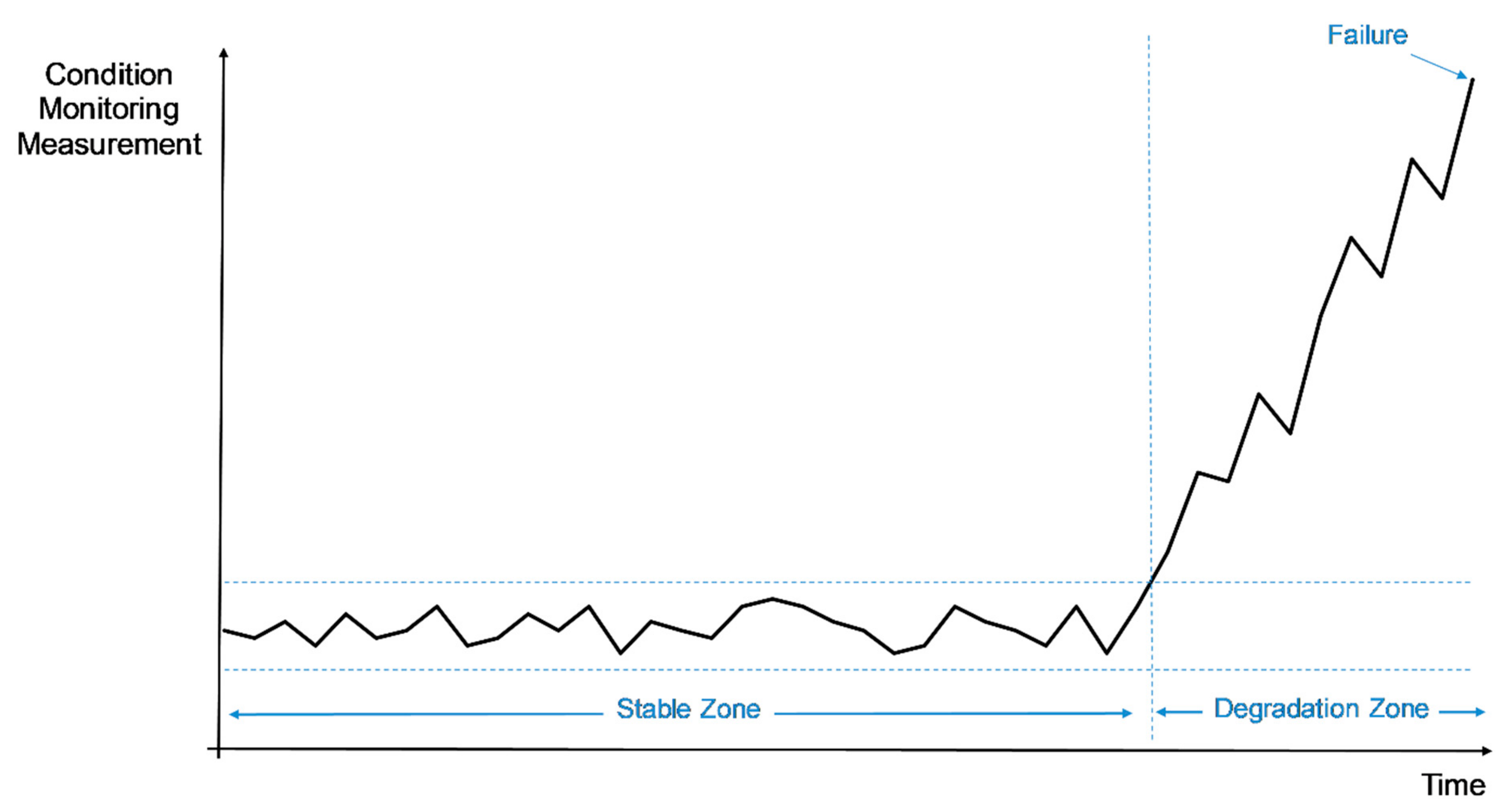
• Predictive maintenance: relies on monitoring and inspection of the equipment for the determination of its operational condition, maintenance interventions will only be carried out if a deviation on the equipment’s normal behavior is detected.

For predictive maintenance to be practiced, however, it is necessary to study and understand the equipment’s behavior throughout its whole lifecycle, from the beginning of its operation to the occurrence of a final failure. According to several authors [37,38], the lifecycle of some machines can be divided into two zones (Figure 3): a first stable zone in which the condition monitoring measurement varies slightly around a mean, and a second degradation zone in which the machine behavior deviates significantly from the normal one [39].

In the proposed method, these two zones will be represented by two different places in the Petri net. In fact, the network developed to represent the conditions of a machine (or piece of equipment) will be composed of five places, as shown in Figure 4. It is worth noting that the Petri net of Figure 4 represents only one machine of a system, not the entire system. These five places are described below:

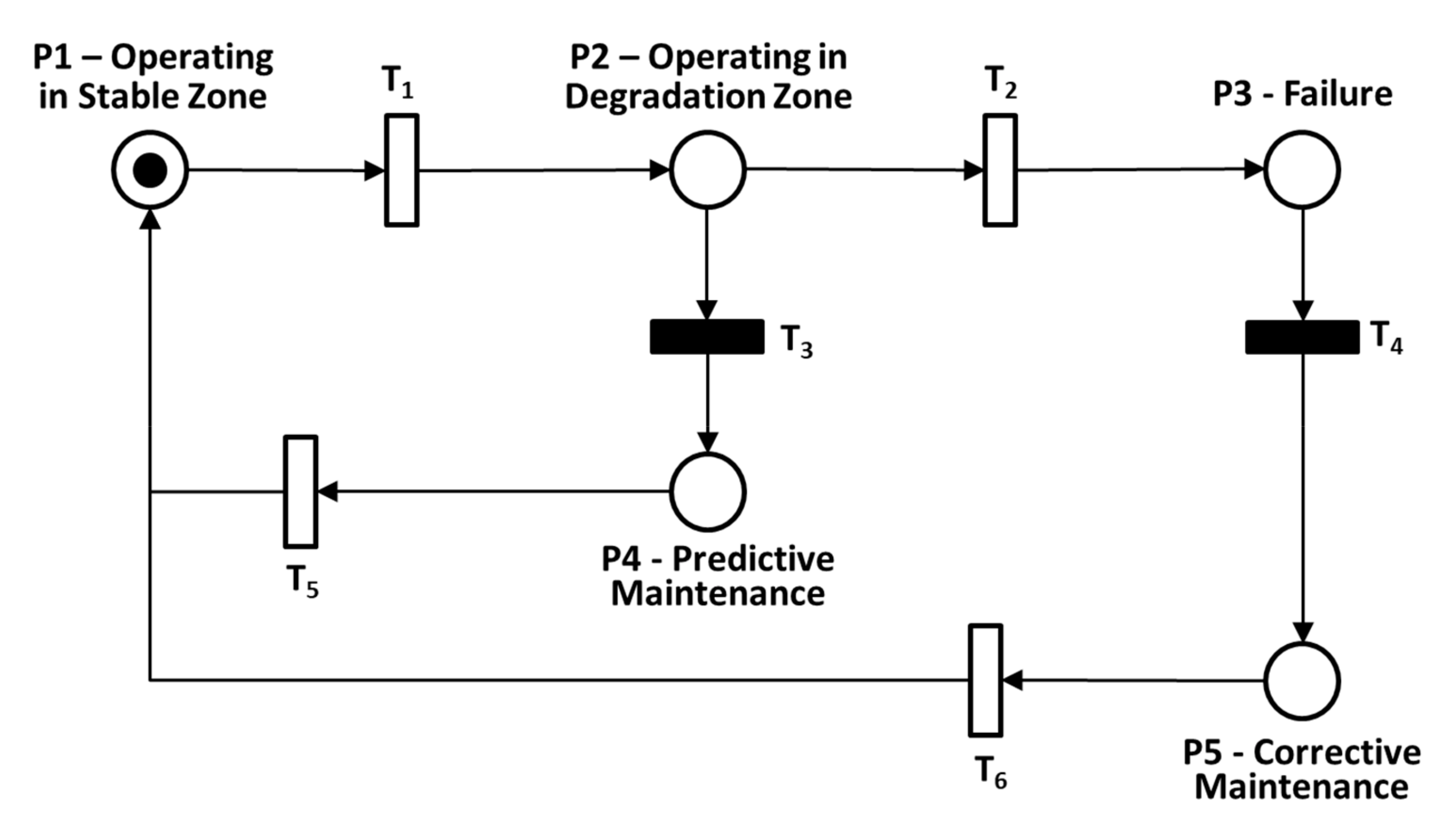
• P1: The machine is operating in the stable zone;
• P2: The machine is operating in the degradation zone and will soon fail;
• P3: The machine has failed and is no longer operable;
• P4: The machine is going through repair before it fails, because it has previously entered in the degradation zone;
• P5: The machine is going through repair after it has failed.

The place where the token is represents the current condition of the machine. In Figure 4, for example, the machine is currently operating in the stable zone. Its condition will change when transition T1 fires, which makes the token move from P1 to P2. When in P2, the token can move to P3 or P4, depending on which transition, T2 or T3, fires. If T2 fires, the token goes to P3, which means the machine has failed and will only go on repair (P5) if T4 fires. But, if T3 fires, the token goes to P4, which means the machine goes on repair before it has failed. The machine goes back to operating in the stable zone (P1) after repair occurs (firings of T5, if the token is in P4, or T6, if the token is in P5). It is worth noting that the proposed Petri net can only represent machines whose degradation pattern is represented in Figure 3. If the degradation pattern of the machine is different from the one presented and can’t be divided into two zones, the Petri net model should be redesigned.

For a better understanding of how transition firings occur, a better description of each transition is made below:

• T1: it is a timed transition that, if fired, makes the token go from P1 to P2, i. e., represents the machine going from the stable zone to the degradation zone. The firing delay is random and based on a probabilistic distribution that represents the time that the machine usually operates in the stable zone;
• T2: it is a timed transition that, if fired, makes the token go from P2 to P3, i. e., represents the machine going from the degradation zone to a failed state. The firing delay is random and based on a probabilistic distribution that represents the time that the machine usually operates in the degradation zone;
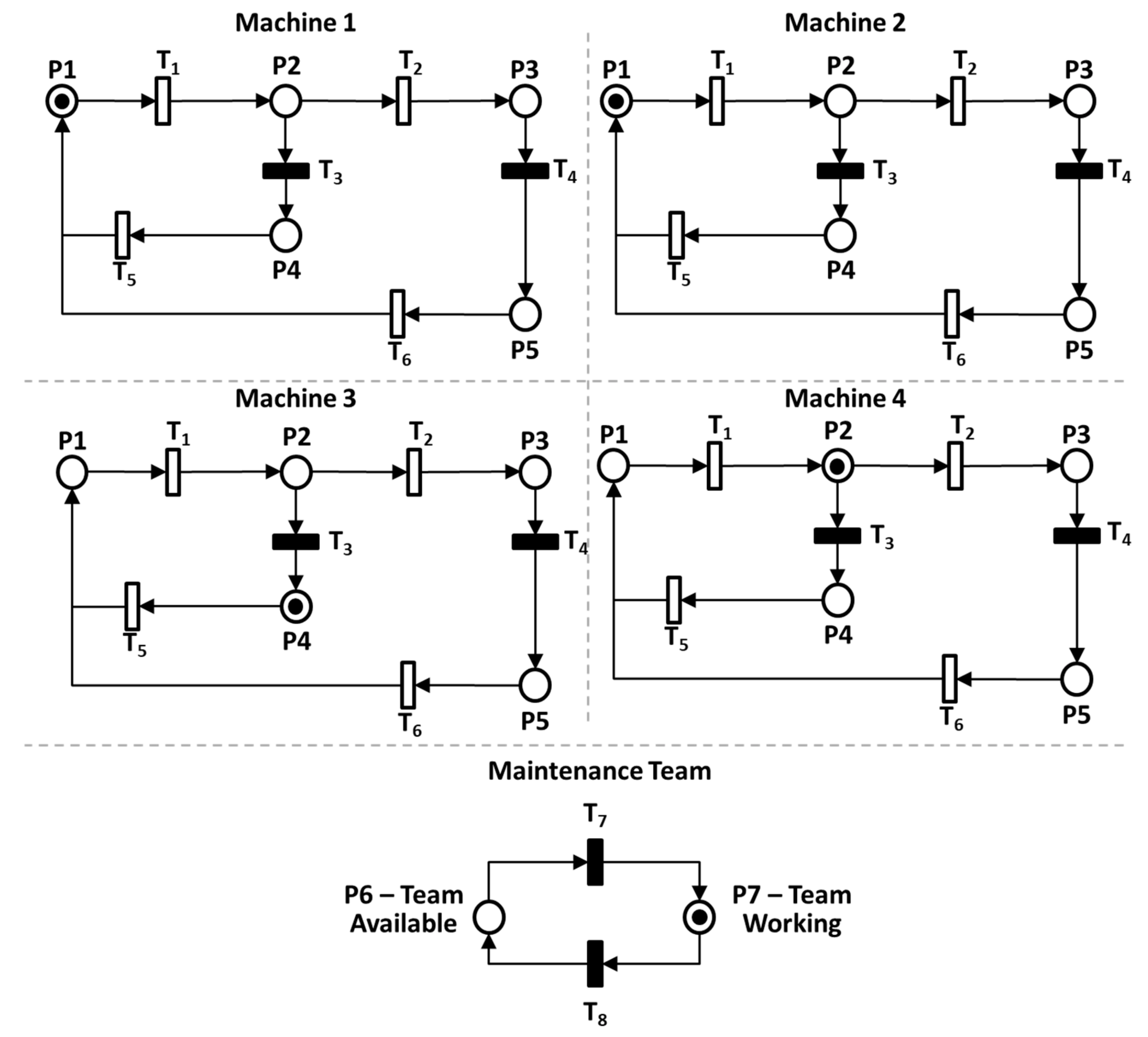
• T3: it is an immediate transition that, if fired, makes the token go from P2 to P4, i. e., represents the machine going from the degradation zone to repair before it fails. Since it is an immediate transition, this means that as soon as the token arrives at P2, it would immediately go to P4, but in the model proposed here, this will only happen if the maintenance team is available to repair the machine;
• T4: it is an immediate transition that, if fired, makes the token go from P3 to P5, i. e., represents the machine going from the failed state to repair. Since it is an immediate transition, this means that as soon as the token arrives at P3, it would immediately go to P5, but in the model proposed here, this will only happen if the maintenance team is available to repair the machine;
• T5: it is a timed transition that, if fired, makes the token go from P4 back to P1, i. e., represents the machine going from repair back to operating in the stable zone. The firing delay is random and based on a probabilistic distribution that represents the time that the machine usually stays in repair;
• T6: it is a timed transition that, if fired, makes the token go from P4 back to P1, i. e., represents the machine going from repair back to operating in the stable zone. The firing delay is random and based on a probabilistic distribution that represents the time that the machine usually stays in repair.

Considering the description of the network of Figure 4 above, particularly the descriptions of transitions T3 and T4, it becomes clear that, in the proposed method, the Petri net should be able to represent multiple machines, as well as the maintenance team activity. For a better understanding of how the complete Petri net model works, let us consider an example of a system with four machines and a maintenance team, as shown in Figure 5.

In the Petri net of Figure 5, Places P6 and P7, as well as transitions T7 and T8, were added to represent the maintenance team activities. Place P6 represents the maintenance team available to do a repair job in one of the machines and P7 represents the maintenance team busy, working on a repair. The immediate transition T7 fires only when there is one machine in the degradation zone or in the failure state. The immediate transition T8 fires only when the machine goes from repair to operating in the stable zone again.

It is possible to notice that Figure 5 is representing a specific state of the system, considering the positions of the tokens. In it, machines 1 and 2 are still operating in the stable zone, machine 3 is being repaired and machine 4 is operating in the degradation zone, while the maintenance team is working (repairing machine 3). If the team was available, machine 4 would already be in maintenance, but in this case it is forced to work in the degradation zone. If the team finishes the repair fast enough (when the token of machine 3 returns to place P1), then machine 4 will be repaired, otherwise it may fail and remain so until the team finishes its work.

Now, using the Petri net model that represents the system under study, it is possible to simulate its operation for a given period of time and compute its availability and reliability, as well as other characteristics of its functioning. But, to do so, it is important to define what availability and reliability are for the system.

Reliability, according to Carazas and Souza [4], is defined as the probability that a system will properly perform its functions during a specified period of time and under a given set of operating conditions. Availability, on the other hand, is defined as the ability of a system (under combined aspects of its reliability and maintenance support) to perform its required function over a period of time. Availability can be expressed by an equation based on system’s uptime and downtime, as follows:

$$\mathit{\text{Availability}} = \frac{\mathit{\text{Uptime}}}{\mathit{\text{Uptime}}+\mathit{\text{Downtime}}}$$

(1)

Both availability and reliability definitions are based on the system performing its function. Therefore, in order to compute both of them through the Petri net, it is important to define how the system loses the ability to fulfill its function. It is worth noting that the Petri net model was created with redundant systems in mind. Redundant systems have components that perform the same function, and if one of them fails, another prevents the whole system from stop working.

In the example of Figure 5, considering that the 4-machine system fulfills its function if only 2 of them are operating, it will only have its reliability and availability compromised if 3 machines are in a state of failure or in maintenance. In the Petri net model, it is possible to verify the number of machines working by counting the number of tokens present in the places dedicated to represent the machine in operation (both in stable and degradation zones). Therefore, in order to obtain the reliability of the system in a given time interval, the Petri net software must, through stochastic simulation of the model, compute the probability of only one of the four tokens stays in places P1 or P2 (i.e., the probability that at some point within a time interval only one out of four machines is operating). To obtain availability, the software must calculate the percentage of the total time interval at which such a scenario can occur.

With the reliability and availability results obtained through the Petri net, it is possible to evaluate if these values satisfy the stakeholders’ needs and what can be done to optimize the operation and maintenance of the system. For a system consisting of several machines that constantly fail, for example, it is possible to evaluate what would be the effect of an increase in the maintenance team. With a larger team, it is possible to perform the repair of more than one machine simultaneously. This will avoid having inoperative units for a long time while waiting for repair. Of course, this increase in maintenance staff comes at a price, and because of this a cost-benefit study is needed.

In the next section, the proposed Petri net will be implemented for a cooling tower of a coal-fired power plant. The probabilistic distributions required for timed transitions will be based on real values of the system under study. Reliability and availability will be calculated for different sizes of maintenance teams (one, two or three machines will be considered to be repaired simultaneously). Finally, a cost-benefit analysis will be undertaken considering the effect that the cooling tower has on the thermal cycle of the plant.

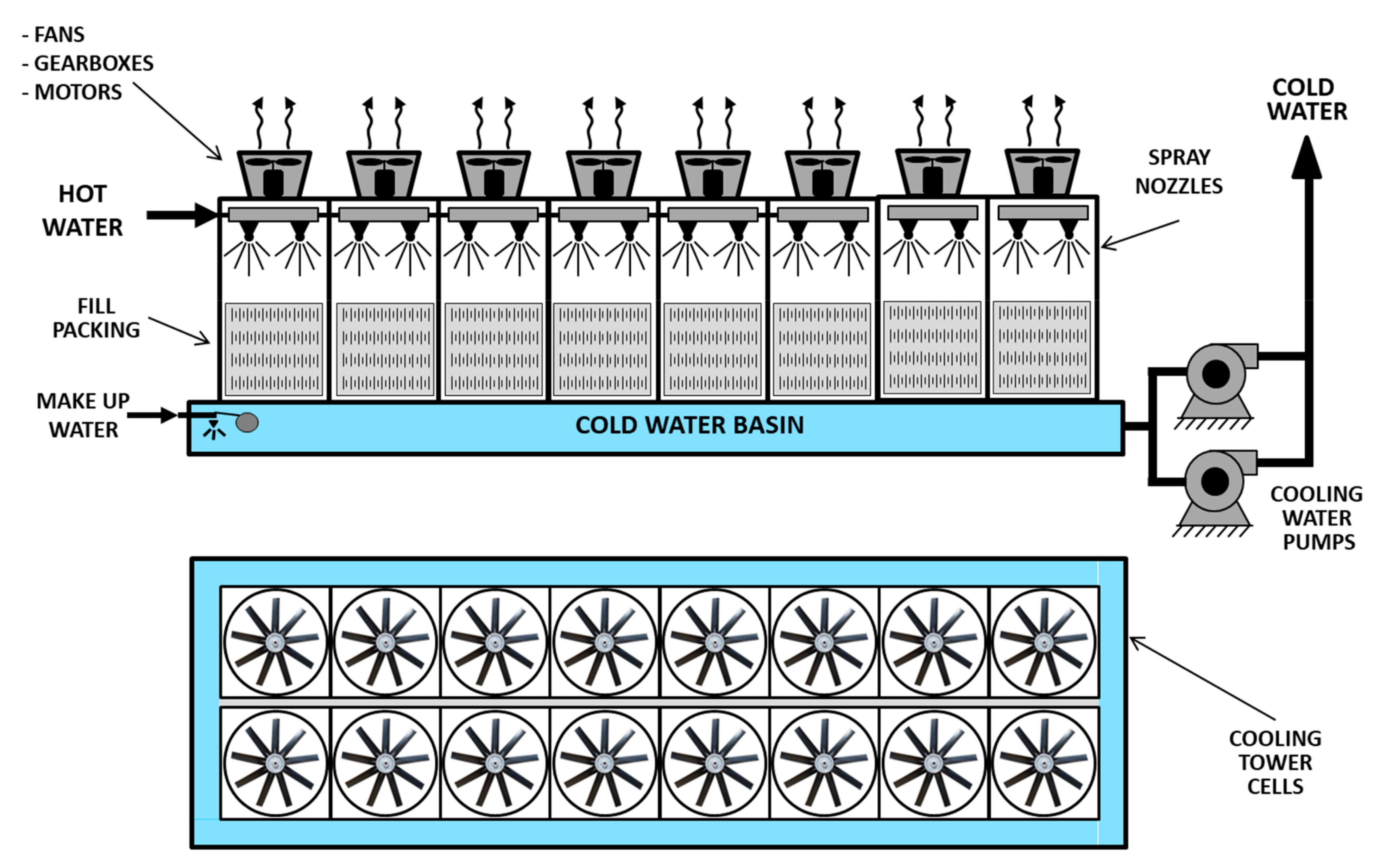
4. Maintenance Strategy Optimization of a Cooling Tower

Figure 6 shows, in a simplified way, how the coal-fired power plant under study generates energy. In the plant, feed water enters the boiler and is transformed into saturated steam by absorbing heat generated by coal burning. This steam is responsible for moving the turbine, which is divided into three stages: low, intermediate and high pressure (LP, IP and HP). The turbine transmits movement to the electric generator, responsible for transforming this movement into electrical power. The steam leaving the LP turbine must be condensed and then fed back into the system. For this condensation to occur, the steam exchanges heat with the cooling water from the cooling tower.

As can be seen, the cooling towers are an integral part of the condensation process. This process, as is well known, is vital to assure thermal power plant efficiency, and is strongly influenced by the control of the inlet cooling water temperature and flow. The cooling water temperature control in turn is achieved by controlling the amount of heat exchange promoted by the cooling tower fans. Because of this, it is common for cooling towers to contain more fans than the minimum required, ensuring that the necessary heat exchange occurs even if some of them fail to operate. However, if too many fans fail at the same time interval, the system’s heat transfer capacity will inevitably be reduced in comparison with design conditions, leading to a reduction in electric power generation. To prevent this from happening, the plant operator will most certainly increase the burning of coal in the boiler. Such a common decision will help meet the power output demand, but causes the decrease of plant efficiency and an increase in CO₂ emissions. Therefore, it seems advisable that maintenance planners should give due attention to the cooling tower subsystem in two respects: prevent degradation, and assure prompt restoration in case of failure.

Figure 7 shows the cooling tower studied in this article, highlighting its main components. As can be seen, the tower has 16 cells, each consisting of a fan, gearbox and motor. According to the original design of this system, only thirteen fans in operation are required to maintain acceptable heat exchange, although a larger number in operation would optimize the thermal cycle. This means that if three fans fail simultaneously, it is still considered that the cooling tower is performing its function properly. If four or more fail, however, it is considered that the system is no longer performing its function, seriously affecting the thermal cycle of the plant.

Keeping cooling tower availability certainly requires an adequate amount of human and material resources. However, determining the ideal size of the maintenance staff, or the right amount of tools, spare parts, etc. is no easy task, particularly in the operation of a large and complex thermal power plant. In addition, it means a significant trade-off between necessary investment on the one hand, and operational profit on the other. In the next section, the developed Petri net model is implemented in the cooling tower described.

4.1. GSPN Model for the Cooling Tower

After analyzing the failure records of the cooling tower’s components during one year of operation of the plant, it was possible to perceive that the gearboxes are the most critical component, as shown on the Pareto chart presented in Figure 8. The registered gearbox failures are related to excessive levels of vibration, usually due to leakage or lack of oil, or some mechanical failure.

Given the failures of this component, the gearboxes present in the cooling tower are already equipped with a monitoring system that can detect the moment the component changes from stable to degraded mode of operation, as shown in Figure 3, and sends a message, called an alarm, to the maintenance team. These condition-based monitoring systems are commercially available and largely described in literature [40,41,42,43], and thus will not be described here. By having this system already installed, however, it was possible to gather information about the time between a cell going into operation and the alarm message being sent, as well as the time between sending the alarm and the gearbox failure and the repair time.

Table 1. Data gathered about the gearbox lifecycle.

Item Number	Time to Alarm (h)	Time between Alarm and Failure (h)	Time to Repair (h)
1	3288	39	139
2	2496	266	82
3	5688	377	189
4	168	1140	230
5	648	331	23
6	1752	341	78
7	3792	65	156
8	816	28	240
9	360	584	201
10	960	161	303
11	3384	142	48
12	1200	118	72
13	792	68	8
14	1152	641	122
15	912	72	187
16	2904	761	144
17	624	322	194
18	552	125	170
19	696	79	198
20	3192	147	205
21	504	123	157

shows the values obtained from 21 well-recorded gearbox failures. Although gearboxes had more failures during one year, only these 21 were still recorded in the monitoring system database and also in the plant asset management system.

The data presented in Table 1 are used to obtain probabilistic distributions that are inserted into the timed transitions of the Petri net (T1, T2, T5 and T6 of Figure 4). This was done by using maximum likelihood estimation (MLE).

MLE is a widespread method used for parameter estimation and it is considered to be a robust parameter estimation technique [44,45]. From a data set and given a statistical model, the estimation by maximum likelihood estimates the best values for the different parameters of the model.

The objective of the MLE is to find the best parameters values of the chosen distribution for a given data set, which is done by maximizing the likelihood function value. The likelihood function is given by the following equation [46]:

$$\mathrm{L}= {\displaystyle \prod }_{\mathrm{i}=1}^{\mathrm{n}}\mathrm{f}\left({\mathrm{x}}_{\mathrm{i}};{ \mathsf{\theta }}_1,{ \mathsf{\theta }}_2, \dots ,{ \mathsf{\theta }}_{\mathrm{k}}\right)$$

(2)

where f represents the probability density function for the distribution, n is the size of the data set, x_i is each data value from the data set and θ₁, θ₂,… θ_k are the parameters of the distribution that need to be estimated.

The parameter values that maximize the value of the likelihood function are found by taking the logarithm of this function and, then, setting the partial derivative of the log-linear equation for each parameter equal to zero [46], as shown in the following equation:

$$\frac{\partial (\ln L)}{\partial {\theta }_j}=0 , j=1, 2, \dots , k$$

(3)

The type of distribution that is used to represent a given phenomenon depends on the phenomenon’s nature. In the field of reliability, the Weibull distribution is very popular for representing asset lifetimes, as well as to model degradation processes [47,48]. A lognormal distribution, on the other hand, is used to model continuous random quantities when the distribution is believed to be skewed, such as the time to repair equipment and lifetime variables [49]. It was decided, therefore, that the time for alarm and the time between alarm and fault will be represented by Weibull distributions and that the time for repair would be represented by the lognormal distribution.

The two parameter Weibull probability density function is written as:

$$f\left(t\right)=\frac{\beta }{\mathsf{\eta }}{\left(\frac{t}{\mathsf{\eta }}\right)}^{\beta -1}{e}^{-{\left(\frac{t}{\mathsf{\eta }}\right)}^{\beta }}$$

(4)

where β is the shape parameter and η is the scale parameter.

The lognormal distribution probability density function is written as:

$$f\left(t\right)=\frac{1}{tS\sqrt{2\pi }}{e}^{-\frac{1}{2}{\left(\frac{lnt-{\mu }_{ln}}{S}\right)}^2}$$

(5)

where μ_ln is the mean of the natural logarithms of the times-to-failure and S is the standard deviation of the natural logarithms of the times-to-failure.

Weibull++ software [50] was used to determine the distribution parameters through MLE. The software can easily generate the log-likelihood function in a three-variable graph. In this graph, the x-axis and the y-axis represent the parameters of the distribution and the z-axis represents the log-likelihood value. The best values for the distribution parameters are found at the peak of the graph, since it is there that the likelihood function has its value maximized. Figure 9, Figure 10 and Figure 11 show the results obtained through the MLE.

From Figure 9, the obtained parameters of the Weibull distribution that best represent the “Time to Alarm” are β = 1.24 and η = 1840. The value of β indicates that failures are typical of aging effects and justify the application of predictive maintenance. From Figure 10, the obtained parameters of the Weibull distribution that best represent the “Time between “Alarm and Repair” are β = 1.08 and η = 292. From Figure 11, the obtained parameters of the Lognormal distribution that best represent the “Time between Alarm and Repair” are μ_ln = 4.78 and S = 0.87.

After determining the parameters of the distributions, it is possible to create the Petri net model for the cooling tower shown in Figure 12. In order to represent the simultaneous repair of more than one component, the figure model contains “three maintenance teams” (A, B and C). This does not mean that three completely separate and independent teams would exist in the plant, but only that, if necessary, the maintenance team would be large enough to repair up to three cells simultaneously. In addition, the simulation was done for different scenarios, that is, considering that only one component could be repaired at a time (one maintenance team), that two could be repaired (two maintenance teams), and finally that three could be repaired simultaneously (three maintenance teams). GRIF [51], a Petri net software, was used to run this model.

It is important to make it clear, before presenting the results obtained by the software simulation, that some simplifications and considerations have been made so that the results of the model are true to reality but at the same time, the method is feasible to implement.

First, only failures in gearboxes are considered because they are the components that fail the most, although the system is more complex. To insert different failure modes in the model, however, would require data currently unavailable, which would make the analysis unfeasible.

Second, the time to repair of a component after it fails is usually greater than the time to repair when it is detected while the component is in the degradation zone (but has still not failed yet). Unfortunately, only the time to repair after a failure was available at the plant. It was considered, therefore, that the repair time of the gearbox still in the degradation zone would be 20% lower on average than the repair after the failure. This means that the Lognormal distribution for the repair still in the degradation zone has parameters μ_ln = 4.56 and S = 0.87.

Finally, when a component is repaired and returns to operation (in the stable zone), the Petri net model considers it to be an “as good as new” component. In fact, a piece of equipment that has undergone a repair will not necessarily behave as new and may have a greater probability of failure. However, it is not possible to determine exactly how the equipment will behave after its repair, although it is common practice to replace the broken equipment with a new one.

These considerations are important so that the limitations of the method become clear in the analysis of results.

After implementing the Petri net developed in the software, the simulations for different maintenance team sizes were performed. Considering, initially, the existence of a maintenance team that can only repair one cell at a time, it was possible to obtain the availability and reliability of the system during one year of operation (8760h). In addition, it was also possible to obtain the period of time during which a given number of cells operate simultaneously. These results are shown in Figure 13.

By analyzing Figure 13, it is possible to see that the asymptotic availability of the cooling tower during a year of operation is about 75%, while its reliability curve drops to less than 5%. It is also possible to conclude that, over a year of operation, the 16 cells operated simultaneously at about 8% of the time (738h), whereas in approximately 36% of the time (3122h) there were 15 cells operating together, in 17 % of the time (1509h) there were 14 cells, and so on.

Considering the existence of a maintenance team large enough to repair two cells simultaneously, the results of the simulation show a significant improvement in the performance of the cooling tower. Its availability has increased to 96% and its reliability curve is above the 30% barrier. Figure 14 shows the results of this simulation.

It can be seen from Figure 14 that, with “two maintenance teams”, the 16 cells are in operation simultaneously for 25% of the time (2190h), a number considerably higher than that presented in the simulation with only one maintenance team. It is also noted that the number of hours in operation with a larger number of dead cells also decreased.

Finally, considering the existence of a maintenance team that is large enough to repair three cells simultaneously, the results of the simulation show a more discrete improvement in the performance of the cooling tower in relation to the previous simulation. Its availability has increased to 99% and its reliability curve is above the 40% barrier. Figure 15 shows the results of this simulation.

With the results obtained by the simulations, the next step of the method was to carry out a cost–benefit analysis in order to verify if an investment for the increase in the maintenance team is economically feasible. To do so, one must understand how the cooling tower affects coal-fired power plant efficiency. In the next section, therefore, a thermodynamic analysis of the plant is carried out, which will subsidize the proposed cost–benefit analysis.

4.2. Thermodynamic Analysis

In order to estimate now the influence of the temperature of the water leaving the cooling tower on the increase of coal consumption, and therefore on its cost, an approximated analysis can be carried out using actual design data applied to the theoretical cycle shown in Figure 16.

Condenser design characteristics are: two passes, single shell, single pressure, surface type, transversal arrangement, with a 39,000 m³/h cooling water flow rate. Cooling water inlet and outlet temperatures are, respectively, Tc_in = 28.4 °C and Tc_out = 38.7 °C.

The condenser effectiveness can be calculated using the following equation:

$$\epsilon = \frac{T{c}_{out}-T{c}_{in}}{T_6-T{c}_{in}}=\frac{10.3}{42.7-28.4}=0.72028$$

(6)

If this effectiveness value is further considered to be constant, as well as the temperature increase of ∆Tc = 10.3 °C across the condenser, the value of T₆ can be obtained, and consequently the vacuum conditions inside the condenser, as Tc_in and Tc_out vary:

$$T_6=T_{Cin}+\left(\frac{\Delta T_c}{\epsilon }\right)=T_{Cin}+14.3$$

(7)

At the cooling tower, the inlet water temperature, T_i, can be considered to be equal to Tc_out, and the outlet water temperature, T_o, will depend on how well the equipment functions and is capable of removing heat from the water. On the other hand, since the water leaving the tower is circulated back into the condenser, plus a certain amount in order to make up for evaporation, it is clear that T_o will have a direct bearing on Tc_in, e.g., as T_o increases, Tc_in and T₆ are also expected to increase and cause a loss of vacuum in the condenser. Values for T_o can be obtained using the following equation:

$$T_0=T_i-\mathsf{\eta }\left({\mathrm{T}}_{\mathrm{i}}-{\mathrm{T}}_{\mathrm{wb}}\right)$$

(8)

where η is the cooling tower efficiency and T_wb is the local wet bulb temperature of air (in the present case equal to 24.4 °C).

The common range of efficiency for this type of cooling tower is between 70%–75%, however, as cells fail this value can be considerably reduced. The pressure increase inside the condenser (vacuum loss) will affect the Rankine cycle efficiency, coal consumption and, therefore, the plant’s operational cost. By assigning increasing values to p₆ it is possible to calculate the decrease in Rankine efficiency for a constant desired output, as well as the extra cost/hour incurred for any specific fuel calorific power. On the other hand, it is also possible to assign decreasing values to η_T (cycle efficiency) and calculate the corresponding values for T_o as both T₆ and p₆ increase.

Considering the Rankine cycle, the following processes can be evaluated:

q_H = m_c × P_c

(9)

where q_H represents the heat transfer to the fluid (heat exchange at constant pressure at the boiler), m_c is the mass of coal and P_c is the calorific value of mineral coal and q_L is the heat transfer from the fluid (heat exchanged with the cooling water entering the condenser which in turn will be further cooled at the cooling tower):

q_L = m × c_p × (T_i − T_o)

(10)

where m is the mass of cooling water, and c_p is the specific heat for water.

The network is written as:

q_H = w_net + q_L

(11)

Equation (11) can now be written as follows:

q_H = w_net + m × c_p × (T_i − T_o) = w_net + m × c_p × T_i − m × c_p × T_o

(12)

By combining Equations (8) and (12), the value of q_H as a function of T_o is defined:

$$q_H=w_{net}-\frac{m·c_p·\mathsf{\eta }}{1-\mathsf{\eta }}·T_{wb}+\frac{m·c_p·\mathsf{\eta }}{1-\mathsf{\eta }}·T_o$$

(13)

Therefore, the amount of coal to be burnt is:

$$m_C=\frac{q_H}{P_C}$$

(14)

It can easily be seen in Equations (13) and (14) that, for any T_wb and a constant value of w_net, an increase in T_o will cause an increase in both q_H and m_c. In other words, an increase in the temperature of the cooling water leaving the cooling tower will cause an extra consumption of coal. Considering the cost of coal, this extra consumption can also be expressed in monetary value:

Cost of fuel = m_C × ($/unit mass of coal)

(15)

Finally, it is possible to correlate T_o and the extra fuel consumption per hour as shown in Figure 17, considering the net power generation of 360 MW.

Taking into account the characteristics of the cooling tower under study and knowing the results of Figure 17, it is possible to predict the consumption of coal per hour depending on the number of cells in operation. Figure 18 shows such results.

It can be seen that the effect of a larger number of cells in operation has a direct impact on the consumption of coal, and consequently on the thermal efficiency of the plant. However, given some limitations in the design of the plant, the consumption of coal cannot exceed the limit of 130.5 tons per hour. This limit exists for safety reasons and to maintain the integrity of the mills and the boiler. This means that if a number greater than three cells fails, it will not be possible to increase the consumption of coal to maintain power generation, as Figure 18 shows. Therefore, the power generated will be compromised, as shown in Figure 19.

Last but not least, since pressure and temperature are not independent variables along condensation processes, it is always good to remember that reductions in condenser vacuum brought about by the increase in condenser temperature can ultimately represent an explosion risk that should never be overlooked.

In the next section, a cost–benefit analysis, comparing the simulation results obtained by the Petri net with the thermodynamic analysis of the plant, will be performed.

4.3. Cost–Benefit Analysis

Table 2. Annual coal consumption by number of maintenance teams.

Number of Operating Cells	1 Repair Team		2 Repair Teams		3 Repair Teams
	Working Time (h)	Coal Consumption (tons)	Working Time (h)	Coal Consumption (tons)	Working Time (h)	Coal Consumption (tons)
16 Cells in Operation	738	95,410	2190	282,948	2453	316,902
15 Cells in Operation	3122	404,973	2716	352,250	3154	409,064
14 Cells in Operation	1509	196,426	2803	364,807	2015	262,205
13 Cells in Operation	1053	137,410	701	91,454	1051	137,182
12 Cells in Operation	782	102,086	175	22,864	88	11,432
11 Cells in Operation	569	74,307	88	11,432	0	0
10 Cells in Operation	986	128,608	88	11,432	0	0
Total	8760	1,139,220	8760	1,137,187	8760	1,136,785

shows the performance of the tower according to the number of maintenance teams, exposing how many hours, over a year, one has a certain number of cells operating simultaneously. In addition, it also shows the total coal consumption in each of these situations. The calculation of coal consumption took into account the results shown in Figure 18, as well as the plant limitations of 130.5 tons/h.

It can be seen from Table 2 that the total coal consumption in the plant when there is only one maintenance crew for the cooling tower is 1,139,220 tons. When there are two teams, this consumption is 2033 tons less (saving 0.17%). With three teams, consumption is 2435 tons lower (saving 0.21%). This amount of coal that is saved is one of the main economic factors in determining whether an investment in the size of the maintenance team will be rewarded. But it is worth remembering that in the situation described, one also gains from the environmental factor, since a considerable amount of coal is no longer being consumed.

It is possible to calculate how much savings the plant makes by increasing the number of maintenance teams.

Table 3. Total of savings with extra maintenance teams.

Costs Description		1 Repair Team	2 Repair Teams	3 Repair Teams
Total costs with coal	Cost per ton (US$/ton)	83.44	83.44	83.44
	Tons of coal consumed (ton/year)	1,139,220	1,137,187	1,136,785
	Total costs with (US$/year)	95,056,527	94,886,853	94,853,303
Costs for buying energy on free market	Average price of MWh on the Brazilian free market (US$)	73.83	73.83	73.83
	MWh bought on the free market	18,960.7	2311.1	290.4
	Total costs with MWh bought (US$/year)	1,399,868	170,629	21,440
Expenses with maintenance teams	Cost of man hour (US$/h)	16	16	16
	Working hours per year of one maintenance technician (h/year)	2080	2080	2080
	Number of maintenance technicians	3	6	9
	Total of Expenses (US$/year)	99,840	199,680	299,520
Total Costs (US$/year)		96,556,236	95,257,162	95,174,263

shows how much is saved, considering the price per ton of coal used in the plant and the man-hour cost of maintenance technicians in the Brazilian context. It should also be taken into account that, by contract, the plant must provide 358 MW of generated power. If the plant is not able to generate enough energy, it must buy the missing energy in the free market to compensate for its inefficiency. According to [52], the average price of MWh in the northeast region of Brazil in 2018 was US$73.83. This need to buy in the free market the extra energy that the plant cannot supply has a considerable impact on the company’s budget. As Figure 19 shows, that situation can occur when 12 or fewer cells are in operation. It is important to remember that Table 1 shows only the costs related to the operation of the cooling tower and those influenced by the size of the maintenance team. Other operating costs of the plant that are not influenced by the operation of the cooling tower are not shown.

In Table 3, three costs are taken into account when comparing the different sizes of the maintenance team: coal costs, costs for the purchase of energy in the free market, and expenses with the maintenance team. Coal costs are obtained by multiplying the cost and quantity of coal consumed (presented in Table 2). The costs of purchasing energy in the free market are obtained by multiplying the average price of this energy in MWh by the quantity that must be purchased (this value is obtained by analyzing the time in which the cooling tower operates with 12 cells or less, in Table 2, and the amount of energy that is no longer produced because of this, in Figure 19). Finally, maintenance team expenses are obtained by multiplying the average man-hour cost of a maintenance technician in Brazil by the number of technicians needed and the number of hours they will work in a year. The total costs are obtained by the sum of the three costs described.

It can be concluded from the results shown in Table 3 that the existence of two or three maintenance teams would result in savings of more than US$1 million, when compared with the results obtained with only one maintenance team.

4.4. Sensitivity Analysis

Even though the timed transitions in the Petri net model were based on probabilistic distributions developed with real data, it is important to note that the quality of the results is extremely dependent on the accuracy of these data. Obtaining such values, in turn, depends on the quality of the information collected by the plant, such as failure reports, sensor readings, etc., and can have an impact on the simulation results.

Therefore, a sensitivity analysis was proposed just to highlight how a change in the probabilistic distributions for the timed transitions can influence final results. Considering a 90% confidence interval in the generation of the Weibull distribution of the time to alarm, for example, it is possible to compute its contour plot, shown in Figure 20, which shows the joint region of the parameters at a specific confidence level. In this chart, it can be seen that β goes from 0.84 to 1.73 and η goes from 1190 to 2770. These represent the 2-sided 90% confidence limits on these parameters. Note that the maximum and minimum β values do not necessarily correspond with the maximum and minimum η values.

In order to perform the sensitivity analysis, several (β, η) pair values were implemented in the Petri net model (instead of the original values from the MLE results, β = 1.24 and η = 1840). Figure 21 shows the variation in the results of availability and reliability when these new parameters were used, considering the existence of only one repair team. It is possible to notice that the two metrics suffer great variation, which means that the performance of the system is extremely dependent on such parameters.

Figure 22 and Figure 23 show the same analysis described above, but now considering the existence of two and three maintenance teams, respectively. It is possible to notice that, although the reliability still suffers a certain variation, in both cases the availability is almost constant. This means that the addition of maintenance teams makes the operation of the system more resilient, that is, the system becomes tolerant to small variations in the distribution parameters.

5. Conclusions

Since the trade-off between equipment availability and the size of maintenance teams constitutes an important issue at large power plants, the authors decided to carry out an in-depth study in order to assess the cost–benefit aspects involved in the operation of the steam-generation plant cooling tower. Accordingly, it was decided to model the cooling tower system with its deterioration and repair team availability characteristics using a GSPN. As with other dynamic systems, the cooling tower displays a complex behavior involving variables of time, repairable components periodically tested, failure to start, and random occurrences, that more accurately describe the systems in practice. The GSPN method proved to be a very effective modeling tool for describing and analyzing the dynamic behavior of the system under scrutiny.

The power of the GSPN model is the interactive mode which allows the observation and analysis of the systems based on the pre-conditions set by the users. After showing the influence of cooling water temperature in the Rankine cycle and the relation between cooling water temperature and coal consumption, one important component of the cooling tower was modeled to test the method. Three experiences were performed to evaluate the proposed approach, i.e., availability was estimated for one, two, and three maintenance teams.

Engineering and maintenance scheduling personnel at power-generation plants need to have a system to aid and support them to make reasonable decisions during critical situations, in order to reduce the delay of restoration after a failure has occurred. The Petri net model presented in this study deals with alarms on the cooling tower cells and allows an evaluation to determine the ideal number of repair personnel available at the plant.

The proposed method can be applied to other systems in a power plant by building Petri net models for each one of the systems. The proposed approach shows that SPNs can be successfully used for availability analysis and that GSPNs are very useful in addressing problems that are difficult to solve by standard approaches such as fault tree or reliability block diagrams analyses. This can help engineers and planners to make decisions regarding solution feasibility, total maintenance time, and system availability.

References

1. IEA. Electricity Information: Overview; IEA: Paris, France, 2018. [Google Scholar]
2. Wróblewski, W.; Dykas, S.; Rulik, S. Selection of the cooling system configuration for an ultra-critical coal-fired power plant. Energy Convers. Manag. 2013, 76, 554–560. [Google Scholar] [CrossRef]
3. Fu, C.; Anantharaman, R.; Jordal, K.; Gundersen, T. Thermal efficiency of coal-fired power plants: From theoretical to practical assessments. Energy Convers. Manag. 2015, 105, 530–544. [Google Scholar] [CrossRef] [Green Version]
4. Carazas, F.G.; Souza, G.F.M. Risk-based decision making method for maintenance policy selection of thermal power plant equipment. Energy 2010, 35, 964–975. [Google Scholar] [CrossRef]
5. Modarresi, M.S.; Xie, L.; Campi, M.; Garatti, S.; Care, A.; Thatte, A.; Kumar, P.R. Scenario-based Economic Dispatch with Tunable Risk Levels in High-renewable Power Systems. IEEE Trans. Power Syst. 2018. [Google Scholar] [CrossRef]
6. Tang, C.; Xu, J.; Sun, Y.; Liu, J.; Li, X.; Ke, D.; Yang, J.; Peng, X. Look-Ahead Economic Dispatch With Adjustable Confidence Interval Based on a Truncated Versatile Distribution Model for Wind Power. IEEE Trans. Power Syst. 2018, 33, 1755–1767. [Google Scholar] [CrossRef]
7. Carazas, F.J.G.; de Souza, G.F.M. Availability analysis of gas turbines used in power plants. Int. J. Thermodyn. 2009, 12, 28–37. [Google Scholar]
8. Carazas, F.J.G.; Salazar, C.H.; Souza, G.F.M. Availability analysis of heat recovery steam generators used in thermal power plants. Energy 2011, 36, 3855–3870. [Google Scholar] [CrossRef]
9. Bhangu, N.S.; Singh, R.; Pahuja, G.L. Reliability centred maintenance in a thermal power plant: A case study. Int. J. Product. Qual. Manag. 2011, 7, 209–228. [Google Scholar] [CrossRef]
10. Krishnasamy, L.; Khan, F.; Haddara, M. Development of a risk-based maintenance (RBM) strategy for a power-generating plant. J. Loss Prev. Process Ind. 2005, 18, 69–81. [Google Scholar] [CrossRef]
11. Khan, F.; Haddara, M.; Khalifa, M. Risk-Based Inspection and Maintenance (RBIM) of Power Plants. In Thermal Power Plant Performance Analysis; Springer Series in Reliability Engineering; Springer: London, UK, 2012; pp. 249–279. [Google Scholar]
12. Ignat, S. Power Plants Maintenance Optimization Based on CBM Techniques. IFAC Proc. Vol. 2013, 46, 64–68. [Google Scholar] [CrossRef]
13. Li, Y.G.; Nilkitsaranont, P. Gas turbine performance prognostic for condition-based maintenance. Appl. Energy 2009, 86, 2152–2161. [Google Scholar] [CrossRef]
14. Melani, A.H.A.; Murad, C.A.; Caminada Netto, A.; de Souza, G.F.M.; Nabeta, S.I. Criticality-based maintenance of a coal-fired power plant. Energy 2018, 147, 767–781. [Google Scholar] [CrossRef]
15. Selvik, J.T.; Aven, T. A framework for reliability and risk centered maintenance. Reliab. Eng. Syst. Saf. 2011, 96, 324–331. [Google Scholar] [CrossRef]
16. Niu, G.; Yang, B.S.; Pecht, M. Development of an optimized condition-based maintenance system by data fusion and reliability-centered maintenance. Reliab. Eng. Syst. Saf. 2010, 95, 786–796. [Google Scholar] [CrossRef]
17. Haghifam, M.R.; Manbachi, M. Reliability and availability modelling of combined heat and power (CHP) systems. Int. J. Electr. Power Energy Syst. 2011, 33, 385–393. [Google Scholar] [CrossRef]
18. Sabouhi, H.; Abbaspour, A.; Fotuhi-Firuzabad, M.; Dehghanian, P. Reliability modeling and availability analysis of combined cycle power plants. Int. J. Electr. Power Energy Syst. 2016, 79, 108–119. [Google Scholar] [CrossRef]
19. Khoshgoftar Manesh, M.H.; Pouyan Rad, M.; Rosen, M.A. New procedure for determination of availability and reliability of complex cogeneration systems by improving the approximated Markov method. Appl. Therm. Eng. 2018, 138, 62–71. [Google Scholar] [CrossRef]
20. Billinton, R.; Allan, R.N. Reliability Evaluation of Engineering Systems; Springer: Boston, MA, USA, 1992; ISBN 978-1-4899-0687-8. [Google Scholar]
21. Melani, A.H.A.; Martha de Souza, G.F.; Murad, C.A.; Caminada Netto, A.; Nabeta, S.I. Petri Net based reliability analysis of thermoelectric plant cooling tower. In Proceedings of the 24th ABCM International Congress of Mechanical Engineering, Curitiba, Brazil, 3–8 December 2017. [Google Scholar]
22. Melani, A.H.A.; Caminada Netto, A.; Murad, C.A.; de Souza, G.F.M.; Nabeta, S.I. Petri Net Based Reliability Analysis of Thermoelectric Plant Cooling Tower System: Effects of Operational Strategies on System Reliability and Availability. In Proceedings of the Joint ICVRAM ISUMA Uncertainties Conference, Florianópolis, Brazil, 8–11 April 2018. [Google Scholar]
23. Reddy, G.B.; Murty, S.S.N.; Ghosh, K. Timed Petri net: An expeditious tool for modelling and analysis of manufacturing systems. Math. Comput. Model. 1993, 18, 17–30. [Google Scholar] [CrossRef]
24. He, X.; Murata, T. High-Level Petri Nets-Extensions, Analysis, and Applications; Elsevier Inc.: Amsterdam, The Netherlands, 2005; ISBN 9780121709600. [Google Scholar]
25. Schruben, L.; Yucesan, E. Transforming Petri Nets into Event Graph Models. In Proceedings of the Proceedings of the 1994 Winter Simulation Conference, Orlando, FL, USA, 11–14 December 1994; pp. 560–565. [Google Scholar]
26. Murata, T. Petri nets: Properties, analysis and applications. Proc. IEEE 1989, 77, 541–580. [Google Scholar] [CrossRef]
27. Patrick, P.; O’Connor, A.K. Practical Reliability Engineering, 5th ed.; Wiley: Hoboken, NJ, USA, 2012. [Google Scholar]
28. Nývlt, O.; Rausand, M. Dependencies in event trees analyzed by Petri nets. Reliab. Eng. Syst. Saf. 2012, 104, 45–57. [Google Scholar] [CrossRef]
29. Mansour, M.M.; Wahab, M.A.A.; Soliman, W.M. Petri nets for fault diagnosis of large power generation station. Ain Shams Eng. J. 2013, 4, 831–842. [Google Scholar] [CrossRef] [Green Version]
30. Lefebvre, D.; Leclercq, E.; El Medhi, S.O. Petri Net Models for Detection, Isolation and Identification of Faults in DES; IFAC: New York, NY, USA, 2009; Volume 42, ISBN 9783902661463. [Google Scholar]
31. Melani, A.H.A.; Silva, J.M.; Silva, J.R.; Souza, G.F.M. de Fault diagnosis based on Petri Nets: The case study of a hydropower plant. IFAC-PapersOnLine 2016, 49, 1–6. [Google Scholar] [CrossRef]
32. Beirong, Z.; Xiaowen, X.; Wei, X. Availability Modeling and Analysis of Equipment Based on Generalized Stochastic Petri Nets. Res. J. Appl. Sci. Eng. Technol. 2012, 4, 4362–4366. [Google Scholar]
33. Thangamani, G. Generalized Stochastic Petri Nets for Reliability Analysis of Lube Oil System with Common-Cause Failures. Am. J. Comput. Appl. Math. 2012, 2, 152–158. [Google Scholar] [CrossRef]
34. Talebberrouane, M.; Khan, F.; Lounis, Z. Availability analysis of safety critical systems using advanced fault tree and stochastic Petri net formalisms. J. Loss Prev. Process Ind. 2016, 44, 193–203. [Google Scholar] [CrossRef]
35. Leigh, J.M.; Dunnett, S.J. Use of Petri Nets to Model the Maintenance of Wind Turbines. Qual. Reliab. Eng. Int. 2016, 32, 167–180. [Google Scholar] [CrossRef]
36. Long, F.; Zeiler, P.; Bertsche, B. Modelling the flexibility of production systems in Industry 4.0 for analysing their productivity and availability with high-level Petri nets. IFAC-PapersOnLine 2017, 50, 5680–5687. [Google Scholar] [CrossRef]
37. Goode, K.B.; Moore, J.; Roylance, B.J. Plant machinery working life prediction method utilizing reliability and condition-monitoring data. Proc. Inst. Mech. Eng. Part E J. Process Mech. Eng. 2000, 214, 109–122. [Google Scholar] [CrossRef]
38. Wang, W. A two-stage prognosis model in condition based maintenance. Eur. J. Oper. Res. 2007, 182, 1177–1187. [Google Scholar] [CrossRef]
39. You, M.-Y.; Li, L.; Meng, G.; Ni, J. Two-Zone Proportional Hazard Model for Equipment Remaining Useful Life Prediction. J. Manuf. Sci. Eng. 2010, 132, 041008. [Google Scholar] [CrossRef]
40. Mba, C.U.; Makis, V.; Marchesiello, S.; Fasana, A.; Garibaldi, L. Condition monitoring and state classification of gearboxes using stochastic resonance and hidden Markov models. Measurement 2018, 126, 76–95. [Google Scholar] [CrossRef]
41. Salameh, J.P.; Cauet, S.; Etien, E.; Sakout, A.; Rambault, L. Gearbox condition monitoring in wind turbines: A review. Mech. Syst. Signal Process. 2018, 111, 251–264. [Google Scholar] [CrossRef]
42. García Márquez, F.P.; Tobias, A.M.; Pinar Pérez, J.M.; Papaelias, M. Condition monitoring of wind turbines: Techniques and methods. Renew. Energy 2012, 46, 169–178. [Google Scholar] [CrossRef]
43. Sheldon, J.; Mott, G.; Lee, H.; Watson, M. Robust wind turbine gearbox fault detection. Wind Energy 2014, 17, 745–755. [Google Scholar] [CrossRef]
44. Ayang, A.; Wamkeue, R.; Ouhrouche, M.; Djongyang, N.; Essiane Salomé, N.; Pombe, J.K.; Ekemb, G. Maximum likelihood parameters estimation of single-diode model of photovoltaic generator. Renew. Energy 2019, 130, 111–121. [Google Scholar] [CrossRef]
45. Balakrishnan, N.; Kateri, M. On the maximum likelihood estimation of parameters of Weibull distribution based on complete and censored data. Stat. Probab. Lett. 2008, 78, 2971–2975. [Google Scholar] [CrossRef]
46. ReliaSoft Corporation Maximum Likelihood Function. Available online: https://www.weibull.com/hotwire/issue33/relbasics33.htm (accessed on 16 January 2019).
47. Yianni, P.C.; Neves, L.C.; Rama, D.; Andrews, J.D. Accelerating Petri-Net simulations using NVIDIA Graphics Processing Units. Eur. J. Oper. Res. 2018, 265, 361–371. [Google Scholar] [CrossRef]
48. Andrews, J.; Prescott, D.; de Rozières, F. A stochastic model for railway track asset management. Reliab. Eng. Syst. Saf. 2014, 130, 76–84. [Google Scholar] [CrossRef]
49. Ferreira, C.; Canhoto Neves, L.; Silva, A.; de Brito, J. Stochastic Petri net-based modelling of the durability of renderings. Autom. Constr. 2018, 87, 96–105. [Google Scholar] [CrossRef]
50. Reliasoft Weibull++. Available online: https://www.reliasoft.com/products/reliability-analysis/weibull (accessed on 1 February 2018).
51. SATODEV GRIF Software. Available online: https://www.satodev.com/ (accessed on 1 February 2018).
52. CCEE Preço Médio da Câmara de Comercialização de Energia Elétrica (R$/MWh). Available online: https://www.ccee.org.br/portal/faces/pages_publico/o-que-fazemos/como_ccee_atua/precos/precos_medios (accessed on 1 January 2019).
Figure 1. Worldwide electricity mix, 2016 (Data from [1]).
Energies 12 01951 g001
Figure 2. Graphical structure model of a simple Petri net.
Energies 12 01951 g002
Figure 3. Typical degradation pattern.
Energies 12 01951 g003
Figure 4. Petri net for one macine.
Energies 12 01951 g004
Figure 5. Petri net of a system with four machines and one maintenance team.
Energies 12 01951 g005
Figure 6. Coal-fired power plant process diagram.
Energies 12 01951 g006
Figure 7. Cooling tower system.
Energies 12 01951 g007
Figure 8. Pareto chart of failure records.
Energies 12 01951 g008
Figure 9. Likelihood surface and distribution parameters (β and η) for “Time to Alarm”.
Energies 12 01951 g009
Figure 10. Likelihood surface and distribution parameters (β and η) for “Time from Alarm to Failure”.
Energies 12 01951 g010
Figure 11. Likelihood surface and distribution parameters (Log-Mean is the value of μln and log-standard deviation is the value of S) for “Time to Repair”.
Energies 12 01951 g011
Figure 12. Generalized stochastic Petri net (GSPN) model for the cooling tower.
Energies 12 01951 g012
Figure 13. Simulation results for the cooling tower operation considering one repair team.
Energies 12 01951 g013
Figure 14. Simulation results for the cooling tower operation considering two repair teams.
Energies 12 01951 g014
Figure 15. Simulation results for the cooling tower operation considering three repair teams.
Energies 12 01951 g015
Figure 16. Ideal Rankine cycle with reheating.
Energies 12 01951 g016
Figure 17. Increase of fuel consumption with increasing cooling tower exit temperature.
Energies 12 01951 g017
Figure 18. Coal consumption and outlet water temperature depending on the number of operating cooling tower cells.
Energies 12 01951 g018
Figure 19. Generated power depending on the number of working cells.
Energies 12 01951 g019
Figure 20. Contour plot, at 90% confidence interval, of the Weibull distribution parameters for the Time to Alarm.
Energies 12 01951 g020
Figure 21. Results of the sensitivity analysis considering one repair team.
Energies 12 01951 g021
Figure 22. Results of the sensitivity analysis considering two repair teams.
Energies 12 01951 g022
Figure 23. Results of the sensitivity analysis considering three repair teams.
Energies 12 01951 g023