A Comparative Study of Time Series Forecasting Methods for Short Term Electric Energy Consumption Prediction in Smart Buildings

Abstract

Smart buildings are equipped with sensors that allow monitoring a range of building systems including heating and air conditioning, lighting and the general electric energy consumption. Thees data can then be stored and analyzed. The ability to use historical data regarding electric energy consumption could allow improving the energy efficiency of such buildings, as well as help to spot problems related to wasting of energy. This problem is even more important when considering that buildings are some of the largest consumers of energy. In this paper, we are interested in forecasting the energy consumption of smart buildings, and, to this aim, we propose a comparative study of different forecasting strategies that can be used to this aim. To do this, we used the data regarding the electric consumption registered by thirteen buildings located in a university campus in the south of Spain. The empirical comparison of the selected methods on the different data showed that some methods are more suitable than others for this kind of problem. In particular, we show that strategies based on Machine Learning approaches seem to be more suitable for this task.

1. Introduction

The rapid economic growth and the increasing population in developing countries are causing the global energy consumption to increase. Despite efficiency gains over the last decades, it is estimated that by 2040 the global energy demand will likely increase nearly 25 percent [1]. According to the International Energy Agency (IEA) [2], developing regions are expected to experience large demand growth between 2017 and 2040, especially countries from Asia and Africa. Under the studied scenario, CO${}_2$ emissions from energy will rise around $10\%$ (from $32.6$ to $35.9$ gigatons). While in developed countries CO${}_2$ emissions are expected to drop by $23\%$, in developing regions they are supposed to rise by $27\%$.

Energy consumption has a significant impact on the environment. CO${}_2$ emissions have been identified as responsible of most of the progressive warming of the Earth [3]. Furthermore, current predictions show that this growing trend will continue. Therefore, the reduction of CO${}_2$ emissions has become the focus of international political, economic and environmental research. To lower the energy consumption and help protect the environment, new energy efficiency policies are being implemented. For example, the current energy plan developed by the European Commission requires European Union’s countries adopt a set of measures to reach an energy efficiency of at least $20\%$ [4]. Despite the fact that many industries contribute to such emissions, the building and building construction sectors are responsible for $36\%$ of total energy consumption and nearly $40\%$ of global CO${}_2$ emissions [5].

In an efficient scenario, several building sub-sectors, such as space heating and cooling, water heating, lighting, etc., have been identified for potential energy savings [5]. In this context, the development of energy consumption prediction models are growing in importance for decision-making to implement energy policies. The forecasting problem is generally divided into three categories, based on the prediction horizon: short-term, medium-term and long-term load forecasting. Short-term forecasting involves prediction horizons going from one hour up to a week while medium-term refers to predictions from one moth up to a year. Finally, long-term predictions are characterized by a prediction horizon of more than a year [6]. Most works address short-term prediction horizon since it achieves higher accuracy than the other horizons.

Nowadays, more and more buildings are equipped with sensors that can measure various aspects of the functioning of a building, including the electric energy consumption registered. Such buildings are called smart buildings. Such measurement can be stored, and thus can provide valuable historical data, which can be organized as time series, and thus could be used to predict future energy demands of the buildings.

Traditionally, time series have been tackled using conventional methods, such as statistical analysis, smoothing techniques and exponential smoothing and regression-based approaches. For example, Sen et al. [7] applied the Auto Regressive Integrated Moving Average (ARIMA) approach for forecasting energy consumption and greenhouse gas emission in Indian pig iron manufacturing organizations. In [8], Chujai et al. analyzed the household electric consumption using the Autoregressive Moving Average (ARMA) and ARIMA models. However, despite their popularity, these models are not able to capture complex interactions from non-linear data. In this case, Machine Learning (ML) approaches have arisen as a suitable approach to handle such complexity. For instance, Bonetto and Rossi [9] applied Support Vector Machines and Neural Networks to energy consumption in households.However, despite the good performance achieved with Machine Learning techniques, they may get stuck in a local optimum, a phenomenon that negatively affects their performances. To overcome this problem, in recent works, many authors are exploring new approaches. In Divina et al. [10], Divina et al. proposed to apply an ensemble approach, while, in [11], Meira and Oliveira introduced a bagging approach of conventional methods (ARIMA and exponential smoothing methods).

In this work, we propose a comparative empirical evaluation of different time series forecasting strategies. In particular, we consider both statistical and ML based approaches to this problem. To validate the techniques, we applied them on a dataset regarding the electricity consumption registered by thirteen buildings located at the Pablo de Olavide (UPO) University campus in Seville, Spain, collected over five and a half years. In the experiments conducted, we aimed at predicting the electric energy consumption with a one day horizon. Predictions were based on historical data, and another objective of the experimentation proposed was to assess an optimal value of the amount of historical data that should be used for this kind of problem. Therefore, we can summarize the contributions of this work as follows:

• Analysis and comparison of the performance of statistical and ML based strategies;
• Establishing the size of the historical window to be used to optimize the predictions; and
• Analysis of the electricity consumption data collected from the smart buildings considered.

Results obtained show that Machine Learning approaches could achieve better results, in particular methods based on bagging and boosting ensemble schemes obtained the best results. Moreover, we found that using historical data relating to more than seven days yielded better predictions.

The rest of the paper is organized as follows. In Section 2, some related works are introduced. Then, the data and the techniques used are described in Section 3. In Section 4, the analysis and discussion of the experiments conducted are presented. Finally, the conclusions and future works are presented in Section 5.

2. Related Works

In the scientific community, there is a growing interest in addressing the forecasting problem in energy-related problems such as electricity consumption, loading and demand for various reasons. For example, as pointed out in [12], to create a healthy and sustainable economy, it is necessary to measure the socio-economic and environmental impact of energy production. Another important aspect is the identification of the different electricity consumption behaviors, which may allow adopting policies according to demand response scenarios [13]. Being able to predict future energy demands would provide several concrete benefits, at both economic and social levels. For example, the ability to balance fluctuations in renewable energy generation would facilitate a greater penetration of renewable resources into the electricity system [14]. On the other hand, we may also improve the economic efficiency by applying real-time prices and reducing costs connected to the generation capacity requirements, reducing at the same time the related CO${}_2$ emissions [15,16].

In the literature, time series analysis is the most popular approach for forecasting demands [17]. Among the most widely used time series forecasting methods, we can find the autoregressive moving average (ARMA) and the autoregressive integrated moving average (ARIMA). ARMA and ARIMA are statistical approaches that have been widely applied to short-term forecasting problem. For example, Abdel-Aal and Al-Garni [18] used, in an early work, ARIMA to forecast monthly electric consumption in the Eastern Province of Saudi Arabia. Chujai et al. [8] compared ARIMA with ARMA on household electric power consumption. ARIMA model was also applied by Shirpa and Shashadri [19] to develop a short-term electric load forecasting model of Karnataka State, India.

Various extensions of ARMA and ARIMA have been proposed to include different aspects affecting a time series: the Auto Regressive Integrated Moving Average with eXternal (or eXogenous) input (ARIMAX), which add explanatory variables; the Seasonal Autoregressive Integrated Moving Average (SARIMA), which supports the direct modelling of the seasonal component of the series; or the Multiplicative Seasonal Autoregressive Integrated Moving Average (MSARIMA), which incorporates independent explanatory variables to SARIMA. The ARIMAX was used by Newsham and Birt in [20] to forecast several hours ahead the power demand for an office building with the objective of obtaining a better response to utility signals and reducing the overall energy use. MSARIMA was applied in [21] by Rallapalli and Ghosh to forecast monthly peak electricity demand from five different regions of India with the aim of achieving a better load management.

Regression based techniques represent another branch of classical methods used in time series forecasting. In particular, linear regression has been extensively applied. For instance, Schrock and Claridge [22] used a linear regression approach to investigate the hourly and daily electrical consumption pattern of a supermarket located 100 miles north-northwest of Houston, Texas. Nowotarski et al. [23] applied a family of regression models trained on different subsets of variables. More specifically, data generated from the Global Energy Forecasting Competition 2014 and ISO New England were used. In [24], Samarasinghe and Al-Hawani compared multiple linear regression with Gaussian Processes on power consumption data from 2008 to 2010 to forecast the values in the next 24 h in Norway. In a more recent work, Rahman et al. [25] proposed a high-precision methodology that included multiple linear regression and simple regression model along with other techniques to forecast the total energy consumption in India.

Other forecasting approaches are based on Machine Learning techniques. Within these approaches, the use of Artificial Neural Networks (ANN) have been extensively and successfully applied. In an early work, Park et al [26] used an ANN to induce the relationship among past, current and future temperatures and loads in the electric load forecasting problem. The model was tested on hourly temperature and load data from the Seattle and Tacoma areas in the period from 1 November 1988 to 30 January 1989, with the objective of predicting 1-h and 24-h ahead values. In another early work, Nizami and Ai-Garni [27] proposed a two-layered fed-forward ANN to study how weather-related features may affect the prediction of monthly electric energy consumption. This approach was tested on data collected from the Eastern Province of the Saudi Arabia between August 1987 and July 1993. In more recent works, ANNs are used to tackle the problem of short-term electrical load forecasting, e.g., [28,29,30,31]).

In addition to ANNs, other Machine Learning techniques have been successfully applied to the problem of energy consumption forecasting. For example, Support Vector Regression (SVR) was applied by Jain et al. [32] to develop an energy forecasting model for a multi-family residential building in New York City. The data used in this work span from 27 August 2012 to 19 December 2012. The model was tested using three different temporal granularities: daily, hourly and 10 min. SVR was also applied by Liu et al. [33] to show its effectiveness in predicting hourly energy consumption of buildings. The popular K-Nearest Neighbour (k-NN) technique was used in [34] to explore the performance of the model for short-term electric energy demand. Other approaches were based on Deep Learning [35,36], Random Forest [37] and Evolutionary Algorithms [38]. Finally, it is worth noting that many of these techniques have been adapted within the big data paradigm. For example, Talavera-Llames et al. [39] adapted the strategy proposed in [34] by Lora et al.

Another strategy that has been used is to combine different strategies to get advantage from the different approaches. For instance, Geng et al. [40] proposed a hybridization of SVR with Chaotic Sequence and Simulated Annealing to forecasting monthly electric load data from northeast China and New York City. Both datasets ranges from January 2004 to October 2005. Fan et al. [41] proposed a novel hybrid method that combines SVR, differential empirical mode decomposition (DEMD) strategy and auto regression (AR) for electric load forecasting. The resulting strategy was tested on two datasets. The first consisting of half-hourly electric load data from the New South Wales while the second one of hourly electric load data from the New York Independent System Operator.

Lately, ensembles approaches have also received considerable attention. Jetcheva et al. [42] proposed an ensemble model based on ANNs for day-ahead electricity load and generation forecasting. The model was tested on data from commercial and industrial sites collected over a period of 10 months ranging from July 2011 to April 2012. In another work, Khairalla et al. [43] introduced a stacking multi-learning ensemble scheme to address the problem of short-term energy consumption forecasting. The proposal was tested on the Global Oil Consumption dataset collected over 52 years (1965–2016). Another example of a stacking ensemble approach can be found in [10]. In this case, Divina et al. applied such an approach to the global short-term energy consumption forecasting problem in Spain.

To get a deeper insight on this topic, we refer the reader to [44], where an exhaustive review of Machine Learning techniques for time series forecasting is presented. Reviews of conventional and Artificial Intelligence methods are presented in [15,45].

3. Materials and Methods

3.1. Data

The time series used in this paper refer to data collected by different sensors installed in 13 buildings located on a university campus in the south of Spain. The selected buildings are equipped with sensors that are able to collect the energy consumption every 15 min. However, for the study presented in this paper, a daily consumption resolution was used. In particular, the data used in this paper cover the daily electric energy consumption registered for the buildings over a period of five and a half years, namely from 1 March 2012 to 31 October 2017.

The campus where the buildings are located consists of 33 buildings. We used only 13 buildings since not all buildings are equipped with sensors for registering the electricity consumption.

Table 1. Description of the selected buildings. The first column presents the year of construction and the year of the refurbishment if was made. The second column present the size in m${}^2$, and finally a short description.

Building	Year (Refurbishment)	Size (m${}^2$)	Description
1	1956 (2005)	75,323	university canteen
2	1956 (2001)	527,277	a four story building with several classrooms and offices
3	1956 (1999)	5231.01	a four story building with several classrooms and offices
6	1956 (1999)	5231.01	a four story building with four large classrooms
7	1958 (2003)	5231.01	a four story building with several classrooms and offices
8	1956 (1999)	1948.16	a two story building with four large classrooms
10	1956 (1999)	5231.01	a four story building with several classrooms and offices
12	1956 (1999)	5231.01	a four story building with several classrooms and offices
14	1956 (1990)	5231.01	a four story building with several classrooms and offices
24	1956 (2007)	9134.93	a three story building with several classrooms and offices
25	2012 (-)	16,281.71	a newly two story building hosting the university library and some classrooms
32	1956 (2005)	2530.78	Administration offices
44	2008 (-)	1752.83	a newly three story built building with research labs, classrooms and offices.

shows a general description of the selected buildings, including the year of construction (and year of refurbishment where applicable), the size and a description of the main purpose of the building.

The geographical location of the campus is characterized by extremely high temperatures, with maximum temperatures exceeding 40 ${}^{°}$C during the summer months, and by relatively mild winters, with minimum temperatures of approximately 0–2 ${}^{°}$C. This climate is termed Mediterranean hot summer climate (Csa) according to the Köppen–Geiger classification.

Table 2. Average temperatures, rainfall and average wind speed in Seville.

Year	Avg. Temp.	Avg. Max. Temp.	Avg. Min. Temp.	Rainfall (mm)	Avg. Wind Sp. (Km/h)
2012	18.7	25.8	12.4	324.13	9.0
2013	18.5	25.3	12.6	425.67	9.9
2014	18.9	25.6	13.3	636.50	9.4
2015	19.1	26.8	13.1	318.46	8.6
2016	19.1	26.0	13.5	626.31	9.4
2017	19.6	27.0	13.2	321.0	8.8

shows average temperatures, average maximum and minimum temperatures, the amount of rainfall and average annual wind speed recorded for the years considered in this paper.

The raw data collected presented missing values. To overcome this issue, the raw data were preprocessed. For each building, we computed the daily average electric energy consumption in Kwh. However, raw data presented missing values on some days and we proceeded to apply a preprocessing step to handle this issue. The steps are summarized as follows: (a) days with missing values corresponding to periods of more than 8 h (either continuous or discontinuous) were discarded; (b) days with missing values corresponding to a continuous period of time corresponding to more than 4 h were discarded; and (c) in the rest of the cases, the missing values were approximated by means of a linear regression method. The same approach was used in the case of missing values corresponding to a period of time of less than 8 h for the period from 00:00 to 08:00. In total, 260 days were discarded, thus the final dataset consists of 1810 days. The final dataset is available upon request.

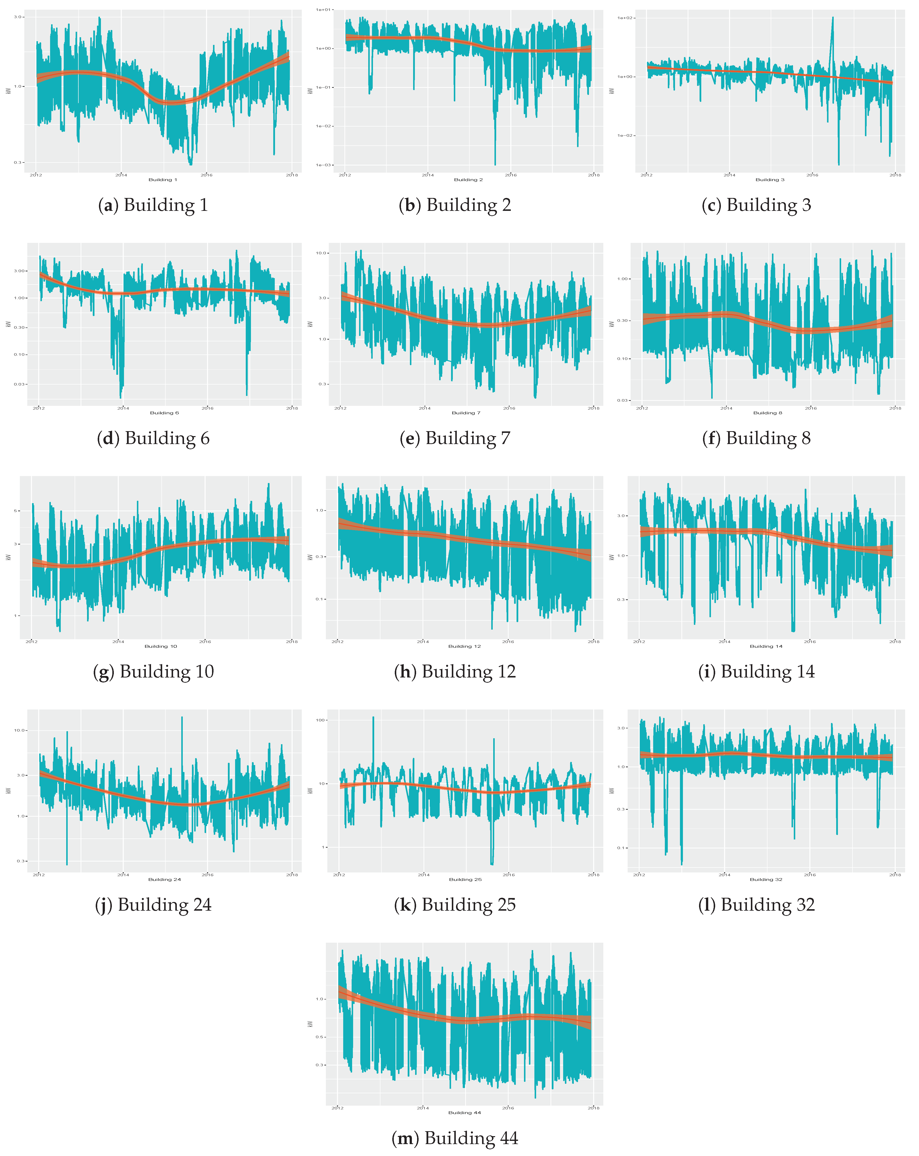
Figure 1 shows the electric consumption and the general trend of each building over the period of time analyzed, scaled using a logarithmic scale in base 10. We used a logarithmic transformation since some significant outliers were present and would have rendered the graphs relative to the original data difficult to read. More specifically, significant outliers are present in buildings 3, 24 and 25. To further analyze such anomalous cases, we checked the temperature registered by Spanish National Agency of Meteorology [46] on such dates. We verified that no sudden changes in the temperatures can justify these anomalous values. Moreover, we verified that there are no records of anomalous operation in the buildings. We decided to maintain such anomalous values to simulate the real functioning of the sensors, and to check in this way the robustness of the techniques to the presence of outliers.

In this way, we could assess the robustness of the various strategies applied to these time series against the presence of outliers, since they are likely to being produce in the normal functioning of sensors.

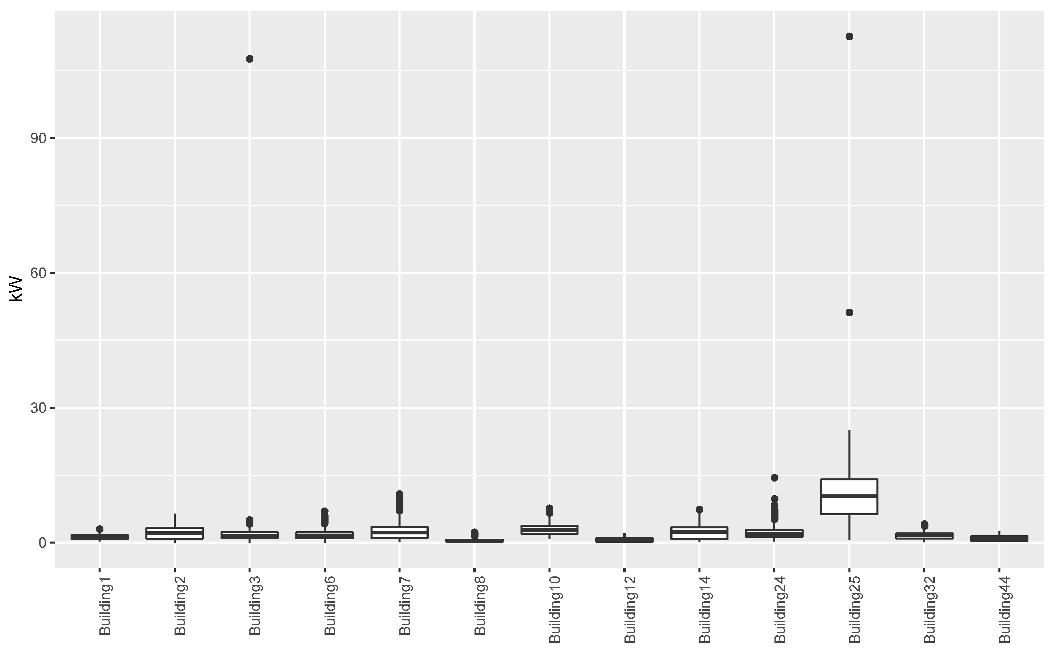
Figure 2 shows the distribution of the values in the final dataset for the buildings considered in this paper. From the results this figure we could confirm the presence of the outliers in the buildings highlighted above. However, we can also notice that there are anomalous values in almost all the buildings, even if their values do not exceed by too much the values considered to be normal. These values may be due to a malfunctioning of the sensors as well as extreme peaks of temperatures. We can also noticed that Building 25 presents a wider distribution of values with a higher average. These aspects could be partially explained by the fact that Building 25 hosts the university’s library, which consists of a huge open space. This, and the particular climatic conditions of south of Spain, implies that this building uses more energy for the heating, ventilation, and air conditioning (HVAC) than other buildings that consist of smaller spaces.

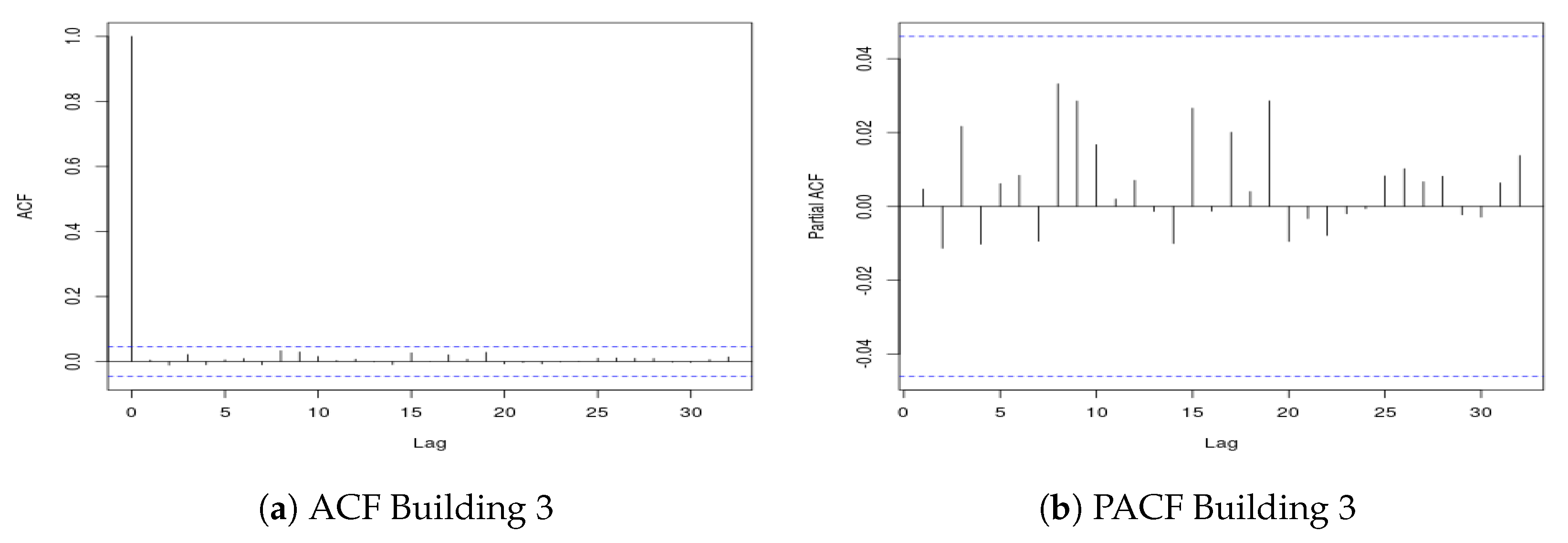
To complete our study of the time series, we performed an analysis aimed at establishing whether the time series used presented stationarity behavior or not. In particular, we performed the Ljung–Box (LB) statistical tests for stationarity [47]. The p-value returned by this test is, in all cases, lower than $0.01$ except for Building 3. To further investigate this case, we present in Figure 3 the the Partial AutoCorrelation Function (PACF) and the AutoCorrelation Function (ACF) pertaining to the data of Building 3. We can notice that in both plots there are no lags that exceed the confidence interval of the ACF and PACF plots, respectively. We can then conclude that Building 3 shows a stationary behavior.

3.2. Methods

In this section, we provide a basic description of the methods used in the experimentation, starting from the classical statistical approaches, namely linear regression and ARIMA. After that, we describe the Machine Learning techniques used in our empirical study.

Linear Regression (LM). Ref. [48] is statistical technique commonly used for time series forecasting. The basic idea behind linear regression is to try to find the relationship between two variables. In its simplest formulation, a linear equation, $Y=a+bX$, is used to represent the association between the independent variable (X) and the dependent one (Y), i.e., the variables to be predicted. In the case where multiple independent variables are used to determine the value of a dependent variable, as is the case of this work, the process is called multiple linear regression. In this case, the goal is to model the linear relation between multiple independent, or explanatory, variables and a dependent variable using an equation such as $Y=a+b_1{X}_1+\dots +b_n{X}_n+ϵ$, where $ϵ$ is the residual (difference between the predicted and the observed value) and $X_i,1\le i\le n$ are the n explanatory variables. For this work, we used the implementation provided by the caret [49] R package.

Auto-Regressive Integrated Moving Average (ARIMA). is a classical method based on Box and Jenkins [50] widely used for time series forecasting, as shown in Section 2. ARIMA is an extension of the simpler AutoRegressive Moving Average (ARMA) that includes the concept of integration. We used this method since it can be used to forecast non-stationary time series. In [51], ARIMA is described as a stochastic model building. In particular, this method can be viewed as an iterative strategy that consists of three steps:

• Identification. In this step, the data and all related information are used for selecting a sub-class of model that might best represent the data.
• Estimation. In a second step, the parameters of the model are trained using the data.
• Diagnostic Checking. Finally, the so-obtained model is validated using the data at disposal and areas where the model can be improved are identified.

ARIMA requires setting three parameters, namely the order of auto-regressive (AR) terms (p), the degree of differencing (d) and the order of moving-average (MA) terms (q). To estimate such parameters for each dataset and each historical window used, we used the arimapar function, part of the TSPred R package [52]. This function returns the parameters of an automatically fitted ARIMA model. The implementation provided by the caret.ts [53] package (an extension for time series models for caret package) was used.

Evolutionary Algorithms (EAs) for Regression Trees (EVTree). EAs [54] are optimization techniques based on the basic concepts of Darwinian evolution. EAs evolve a population of candidate solutions over a number of generations by means of the application of genetic operators, such as selection, crossover and mutation. Each candidate solution, i.e., an individual of the population, is assigned a quality score, or fitness. Usually, EAs start from a randomly initialized population, which is then evaluated to assign a fitness to each individual. A number of individuals are then selected, usually based on the fitness. Crossover and mutation operators are used to generate new individuals starting from the selected ones. The so-generated offspring are then inserted into the population. The whole process is repeated until a stopping criterion is met, e.g., when a maximum number of generations have been performed. The particular EA provided by the EVTree [55] R package was used. This algorithm evolves regression trees [56], i.e., trees used to predict a continuous value based on a set of predictor variables.

Generalized Boosted Regression Models (GBM). [57,58]. This is an ensemble algorithm, where a set of regression trees is trained following a sequential procedure. During this sequential procedure, GBM applies a gradient descend procedure, which is repeated until a given number of trees has been built or when no improvement is detected. The last condition is checked by using the set of current trees to produce predictions. Such predictions are also used to correct the model, so that mistakes obtained in previous iterations can be corrected. A known issue in gradient boosting is overfitting. GBM tackles this problem by using regularization methods, which basically penalize various parts of the algorithm. To produce the final prediction a voting mechanism, among all the tree obtained, is used. We used the GBM implementation provided by the caret R package.

Artificial Neural Networks (ANNs). In a rough analogy of biological learning system, ANNs consist of densely interconnected units, called neurons. Each neuron receives a number of real valued input, e.g., from other neurons of the network, and produces a single real valued output. The output depends on an activation function used in each unit, which introduce non-linearity to the output. However, the activation function is used only if the input received by a unit is higher than a given activation threshold. If this is not the case, then no output is produced. Normally, an ANN consists of different layers of neurons. Among such layers we can distinguish the input and output layers, and in between there may be one or more hidden layers. As said before, there is an activation threshold used in the network, which is determined by weights that are adjusted during a training phase. Several types of ANNs have been proposed. Among these, the simplest, and one of the most widely used one, is the so-called feedforward ANN. In these type of networks, neurons of adjacent layers are connected, and each of these connections is assigned a weight. The information advances from the input layer toward the output layer, which consists of only one unit. The output unit produces the final prediction of the network. The caret package implementation was used.

Random Forests (RF). were first proposed by Breinman and Cutle in [59]. Similar to GBM, RF is also an ensemble approach, where a set of trees are used to produce the final output, using a voting scheme. Each tree is induced from a randomly selected training subset and using also a randomly selected subset of features. This implies that the trees depend on the values of an independently sampled input dataset, using the same distribution for all trees. In the case of regression, the final prediction is represented by the average of the predictions of each induced tree. In addition, for this method, the implementation provided by caret was used.

Ensemble. This method was proposed by Divina et al. [10]. It is a stacking ensemble scheme. In particular, two layers are used to make a final prediction. In the first layer, EVTree, RF and NN are used, and the predictions made by these three methods are then combined on the top layer by GBM to produce the final output. This method shows excellent performances on a problem regarding the prediction of the global energy demands, this it is interesting to check its validity also in the case of a local energy demand setting, such as the one used in this paper.

Recursive Partitioning and Regression Trees (RPart). [60]. This method is based on the CART algorithm, and builds regression trees, using a two states strategy. The resulting model can be represented as a binary tree, which can be easily interpreted. In the first step, the algorithm determines the variable which best splits the data into two groups. For regression, as in this case, the attribute with the largest standard deviation reduction is considered the best and is used for building the decision node. The data are then separated according the the attribute selected, and the process is applied separately to each sub-group determined in the first phase, until the subgroups either get to a minimum size or no improvement can be achieved. In a second step, the obtained full tree is pruned using a cross-validation strategy. Again, the caret implementation was used.

Extreme Gradient Boosting (XGBoost). [61]. This method is similar to GBM, as it shares with it the principle of gradient boosting for building an ensemble of trees. There are, however, important differences. For instance, XGBoost controls over-fitting (a known issue in GBM) by adopting a more regularized model formalization. This allows XGBoost to generally obtain better performance than GBM. XGBoost has recently received much attention in the data science community, as it has been successfully applied in different domains. This popularity is mostly due to the scalability of the method. In fact, XGBoost can run up to ten times faster than other popular approaches on a single machine. Moreover, it is also capable of scaling to billions of instances in distributed or memory-limited settings. The latter feature is achieved via different systems and algorithmic optimizations. Some of this improvements include a novel tree induction algorithm for managing sparse data and a strategy that makes it possible to handle the weights of the instances in approximate tree learning. Parallel and distributed computing makes learning faster, allowing a faster model exploration. Additionally, XGBoost employs out-of-core computation, which enables to process massive date even of a simple desktop. We used the implementation provided by the caret R package.

All the methods used in this study have various configuration parameters. To set the different parameters of the methods, we ran a grid search, exploring the standard parameter values that are used in similar literature.

4. Results

In this section, we present the results obtained by the different techniques described in Section 3.2 on the datasets presented in Section 3.1 and draw the main conclusions. The aim of the experimentation performed was two folds. Firstly, we wanted to assess which technique is more suitable for predicting short term electric energy consumption in a local setting, such in smart buildings. Secondly, we wanted to find an optimal value for the amount of historical data that should be used to obtain good forecasts.

To measure the performances of the different strategies used, we used the Mean Absolute Error (MAE) and the Root Mean Squared Error (RMSE). The measures are defined as follows:

$$\mathrm{MAE}=\frac{1}{n}{\displaystyle \sum _{i=1}^n}|Y_i-{\widehat{Y}}_i|$$

(1)

$$\mathrm{RMSE}=\frac{1}{n}\sqrt{{\displaystyle \sum _{i=1}^n}{(Y_i-{\widehat{Y}}_i)}^2}$$

(2)

where ${\widehat{Y}}_i$ and $Y_i$ are the predicted and the real values, respectively. These two measures are commonly used when assessing the performances of a technique on time series forecasting (see, for instance [62,63]). The advantage of these two measures is that the average forecast error of a model is expressed in the same units of the variable to be predicted. The two measures can assume values greater than or equal to 0, and lower values are considered better. MAE expresses the absolute error, thus it is easy to understand. RMSE assigns high penalties to large errors, since the prediction errors are squared. It follows that the RMSE can be useful when we want abstain from large forecasting errors.

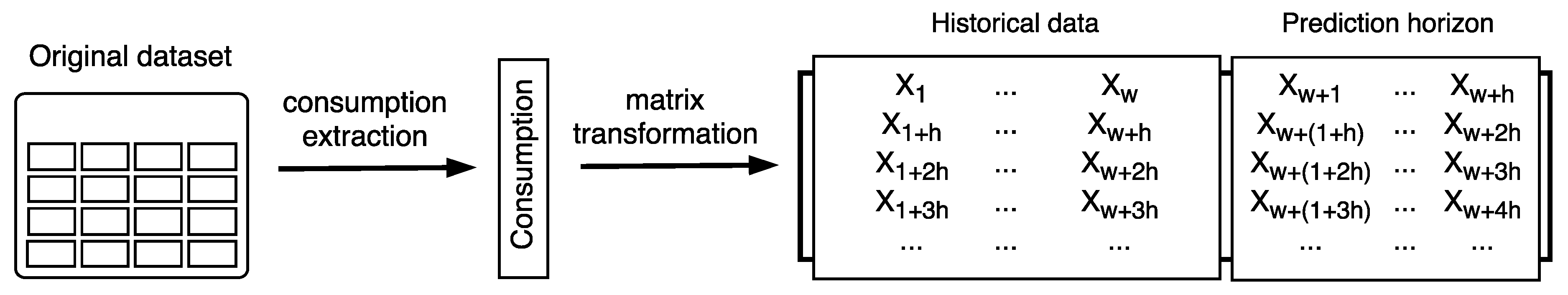
To be used in the proposed experimentation, the original datasets were transformed. The particular preprocessing steps are those used by Torres et al. [36], and are graphically shown in Figure 4. The preprocessing phase can be summarized in two steps. Firstly, we extracted the attribute representing the energy consumption, and as a result a vector of consumption data was obtained. Secondly, a matrix was built using the vector obtained in the first step and according to a historical window, w, and a prediction horizon, h. Notice that w represents the number of historical values that are taken into account so as to induce a predictive model. The obtained model was used to forecast subsequent values (h). In our study, we were interested in predicting the consumption of one day, thus h was set to 1.

Moreover, since one of the aims of the experimentation was to find an optimal value of w, different values of historical window were tested. Specifically, we used historical windows of $7,10,15$ and 20 days. We also tested historical window sizes of multiples of 7, which are common in these kinds of problems, since they usually allow capturing seasonal patterns. However, in this case, the results obtained with such values are not better than those obtained with the above mentioned values, and thus are not included in this paper. This was probably due to the high number of days discarded in the preprocessing of raw data (described in Section 3.1).

The resulting datasets were split in two groups: training set and test set. In particular, we used $70\%$ of the data as training set, and the remaining $30\%$ as test set. Thus, the methods were used to induce a prediction model using the training set, and the forecasting capabilities of the models were assessed on the test set.

Table 3. Results obtained by all the methods on all the buildings for each value of the historical window considered.

		ARIMA		LM		EvTree		RF		NN		GMB		rpart		ENSEMBLE		XGBoost
	w	MAE	RMSE	MAE	RMSE	MAE	RMSE	MAE	RMSE	MAE	RMSE	MAE	RMSE	MAE	RMSE	MAE	RMSE	MAE	RMSE
Edificio 1	7	0.57	0.71	0.50	0.58	0.48	0.58	0.48	0.56	0.49	0.57	0.49	0.57	0.51	0.60	0.55	0.67	0.49	0.57
	10	0.52	0.63	0.46	0.54	0.50	0.61	0.47	0.55	0.46	0.54	0.46	0.55	0.50	0.58	0.51	0.64	0.46	0.55
	15	0.52	0.63	0.46	0.54	0.48	0.58	0.48	0.55	0.46	0.54	0.47	0.55	0.52	0.59	0.54	0.66	0.47	0.55
	20	0.55	0.68	0.47	0.55	0.49	0.59	0.48	0.56	0.47	0.54	0.47	0.55	0.52	0.60	0.53	0.65	0.48	0.56
Edificio 2	7	2.10	2.57	1.37	1.55	1.41	1.61	1.35	1.53	1.40	1.61	1.35	1.53	1.39	1.57	1.41	1.69	1.35	1.54
	10	1.73	2.16	1.31	1.50	1.34	1.57	1.32	1.50	1.32	1.50	1.30	1.50	1.38	1.57	1.41	1.70	1.31	1.51
	15	1.52	1.89	1.32	1.53	1.38	1.63	1.33	1.51	1.33	1.53	1.30	1.53	1.39	1.57	1.39	1.72	1.33	1.54
	20	1.66	2.05	1.32	1.53	1.36	1.61	1.33	1.51	1.33	1.53	1.32	1.53	1.39	1.57	1.35	1.64	1.32	1.54
Edificio 3	7	1.07	4.72	1.07	4.72	1.06	4.67	1.01	4.64	1.09	4.67	1.03	4.65	1.05	4.66	1.04	4.56	1.02	4.65
	10	1.06	4.92	1.06	4.92	0.97	4.63	0.93	4.64	0.91	4.65	0.91	4.64	1.00	4.66	1.02	4.66	0.92	4.64
	15	1.16	5.14	1.16	5.14	0.96	4.68	0.94	4.66	0.93	4.68	0.91	4.66	1.00	4.67	0.98	4.67	0.93	4.66
	20	1.16	5.14	1.16	5.14	0.99	4.68	0.94	4.67	0.93	4.69	0.93	4.67	0.99	4.68	1.02	4.68	0.94	4.67
Edificio 6	7	1.83	2.34	0.96	1.25	0.98	1.29	0.94	1.24	0.97	1.26	0.97	1.28	0.95	1.23	1.00	1.35	0.98	1.28
	10	1.32	1.74	0.88	1.15	0.88	1.20	0.87	1.15	0.87	1.14	0.87	1.16	0.89	1.17	0.91	1.26	0.86	1.16
	15	1.13	1.48	0.88	1.16	0.91	1.25	0.87	1.17	0.89	1.17	0.86	1.18	0.91	1.20	0.93	1.28	0.89	1.19
	20	1.17	1.51	0.88	1.17	0.95	1.26	0.87	1.17	0.89	1.17	0.88	1.19	0.91	1.20	0.93	1.26	0.87	1.18
Edificio 7	7	2.34	2.89	1.13	1.32	1.16	1.41	1.09	1.28	1.12	1.31	1.09	1.30	1.12	1.31	1.13	1.36	1.09	1.30
	10	2.25	2.76	1.06	1.25	1.08	1.32	1.04	1.22	1.06	1.27	1.03	1.21	1.08	1.29	1.13	1.39	1.04	1.24
	15	1.06	1.26	1.06	1.26	1.08	1.28	1.05	1.22	1.08	1.26	1.03	1.21	1.09	1.26	1.11	1.34	1.04	1.22
	20	1.06	1.30	1.06	1.25	1.09	1.32	1.06	1.23	1.07	1.24	1.06	1.24	1.10	1.27	1.12	1.37	1.05	1.22
Edificio 8	7	0.39	0.49	0.36	0.44	0.37	0.46	0.35	0.44	0.36	0.44	0.36	0.45	0.36	0.44	0.39	0.52	0.35	0.45
	10	0.47	0.60	0.34	0.43	0.36	0.46	0.34	0.43	0.34	0.43	0.33	0.43	0.36	0.44	0.38	0.53	0.34	0.43
	15	0.36	0.45	0.34	0.43	0.36	0.47	0.34	0.43	0.34	0.43	0.34	0.43	0.36	0.44	0.37	0.50	0.34	0.43
	20	0.34	0.43	0.34	0.43	0.35	0.46	0.34	0.43	0.34	0.43	0.34	0.43	0.36	0.44	0.38	0.51	0.34	0.43
Edificio 10	7	1.38	1.71	1.02	1.25	1.02	1.28	1.02	1.26	1.02	1.26	1.01	1.24	1.07	1.37	1.07	1.32	1.02	1.26
	10	1.23	1.52	0.95	1.16	0.96	1.21	0.96	1.19	0.94	1.16	0.94	1.17	1.01	1.29	1.02	1.27	0.94	1.18
	15	1.01	1.27	0.97	1.17	0.97	1.21	0.97	1.19	0.97	1.18	0.94	1.15	1.01	1.27	1.03	1.30	0.95	1.17
	20	1.18	1.48	0.98	1.18	0.99	1.23	0.97	1.19	0.97	1.18	0.95	1.16	1.01	1.27	1.04	1.27	0.96	1.18
Edificio 12	7	0.52	0.65	0.39	0.45	0.39	0.46	0.37	0.43	0.38	0.45	0.37	0.43	0.39	0.45	0.40	0.50	0.36	0.43
	10	0.42	0.52	0.37	0.43	0.39	0.47	0.36	0.43	0.37	0.43	0.35	0.43	0.39	0.46	0.39	0.49	0.35	0.43
	15	0.43	0.53	0.37	0.43	0.38	0.46	0.36	0.43	0.37	0.43	0.36	0.43	0.39	0.46	0.38	0.48	0.36	0.44
	20	0.51	0.64	0.37	0.43	0.39	0.47	0.36	0.43	0.37	0.43	0.36	0.42	0.39	0.46	0.39	0.49	0.36	0.44
Edificio 14	7	1.87	2.21	1.19	1.45	1.23	1.51	1.09	1.33	1.17	1.43	1.12	1.36	1.27	1.52	1.24	1.52	1.15	1.39
	10	1.11	1.37	0.98	1.19	1.10	1.39	0.97	1.18	1.01	1.23	0.95	1.14	1.21	1.43	1.03	1.29	0.95	1.15
	15	0.90	1.09	0.89	1.07	1.00	1.23	0.94	1.14	0.90	1.08	0.89	1.09	1.04	1.26	0.94	1.20	0.89	1.09
	20	1.06	1.31	0.89	1.07	1.00	1.23	0.94	1.14	0.90	1.08	0.90	1.10	1.04	1.26	1.03	1.31	0.91	1.10
Edificio 24	7	1.20	1.56	0.94	1.22	0.98	1.27	0.93	1.20	0.95	1.23	0.92	1.20	0.94	1.22	1.02	1.32	0.94	1.21
	10	1.12	1.47	0.88	1.14	0.98	1.30	0.88	1.15	0.85	1.11	0.88	1.14	0.92	1.20	1.00	1.31	0.88	1.15
	15	1.25	1.63	0.87	1.14	0.95	1.25	0.88	1.14	0.88	1.16	0.90	1.17	0.92	1.18	0.94	1.22	0.88	1.16
	20	0.99	1.28	0.88	1.14	1.00	1.32	0.89	1.15	0.88	1.16	0.92	1.19	0.90	1.17	0.96	1.27	0.91	1.18
Edificio 25	7	4.34	5.54	3.48	4.29	3.86	4.94	3.43	4.24	3.73	4.56	3.44	4.28	3.51	4.29	4.01	5.07	3.41	4.26
	10	6.41	7.73	3.29	4.06	3.62	4.56	3.24	4.05	3.47	4.23	3.26	4.09	3.38	4.18	3.82	4.78	3.24	4.07
	15	3.83	4.84	3.33	4.12	3.84	4.83	3.34	4.16	3.49	4.32	3.40	4.29	3.76	4.73	3.70	4.79	3.41	4.29
	20	4.27	5.23	3.33	4.12	3.75	4.73	3.33	4.14	3.47	4.32	3.38	4.21	3.76	4.74	3.72	4.80	3.40	4.25
Edificio 32	7	0.66	0.80	0.52	0.63	0.56	0.69	0.52	0.63	0.53	0.64	0.52	0.64	0.53	0.63	0.59	0.75	0.52	0.63
	10	0.86	1.06	0.51	0.62	0.56	0.69	0.51	0.62	0.51	0.62	0.51	0.63	0.52	0.63	0.58	0.75	0.51	0.62
	15	0.63	0.78	0.52	0.62	0.56	0.70	0.51	0.62	0.52	0.62	0.51	0.63	0.53	0.64	0.55	0.70	0.52	0.65
	20	0.59	0.72	0.52	0.63	0.54	0.66	0.52	0.63	0.52	0.63	0.51	0.63	0.53	0.64	0.57	0.72	0.53	0.64
Edificio 44	7	0.55	0.68	0.46	0.56	0.47	0.57	0.45	0.54	0.47	0.57	0.45	0.55	0.46	0.55	0.49	0.61	0.46	0.55
	10	0.60	0.74	0.45	0.54	0.47	0.58	0.45	0.53	0.45	0.54	0.44	0.54	0.46	0.55	0.49	0.61	0.45	0.54
	15	0.44	0.53	0.45	0.53	0.48	0.59	0.45	0.53	0.45	0.53	0.45	0.53	0.47	0.55	0.50	0.63	0.45	0.54
	20	0.67	0.82	0.45	0.53	0.49	0.59	0.45	0.53	0.45	0.53	0.45	0.53	0.46	0.55	0.48	0.61	0.45	0.54
Average	7	1.45	2.07	1.03	1.52	1.08	1.60	1.00	1.49	1.05	1.54	1.01	1.50	1.04	1.53	1.10	1.63	1.01	1.50
	10	1.47	2.09	0.96	1.46	1.02	1.54	0.95	1.43	0.97	1.45	0.94	1.43	1.01	1.50	1.05	1.59	0.94	1.44
	15	1.10	1.66	0.97	1.47	1.03	1.55	0.96	1.44	0.97	1.46	0.95	1.45	1.03	1.53	1.03	1.58	0.96	1.46
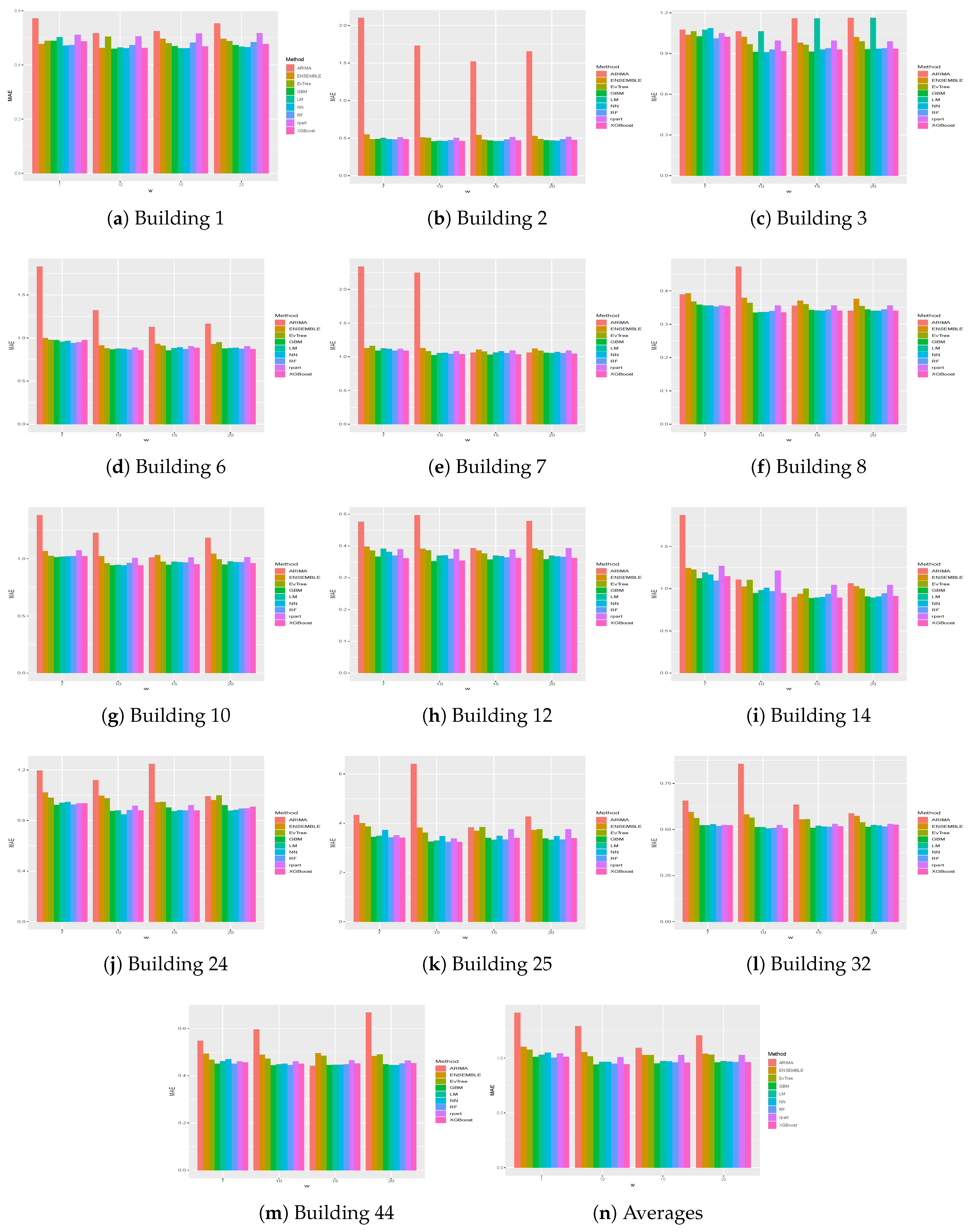
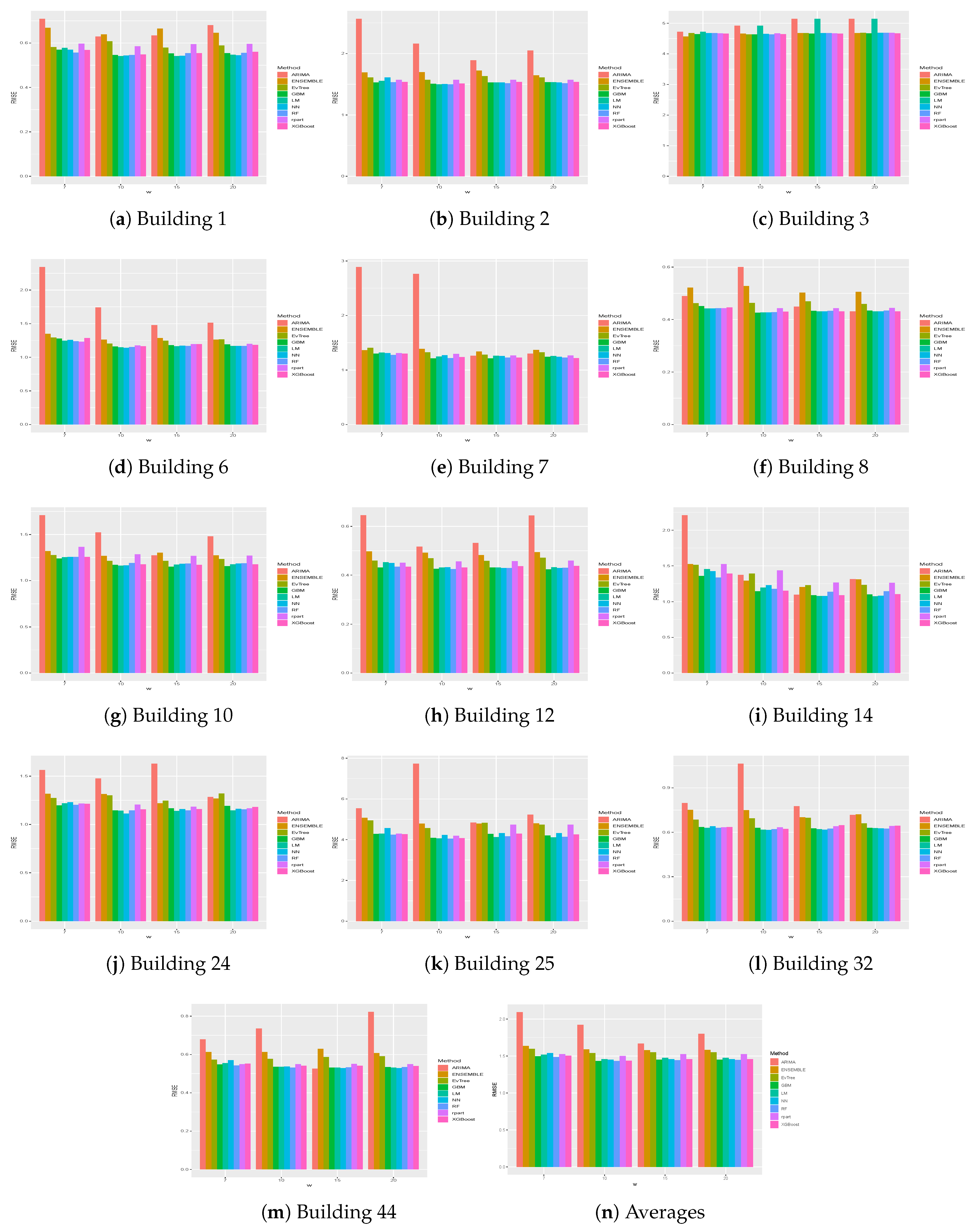
	20	1.17	1.74	0.97	1.47	1.03	1.55	0.96	1.44	0.97	1.46	0.96	1.45	1.03	1.53	1.04	1.58	0.96	1.46

presents the MAE and RMSE obtained on the different buildings for the different historical windows used. In particular, in the last row, the averages results obtained on all the buildings by the different methods are shown. The same results are presented graphically in Figure A1 and Figure A2.

One thing that we can notice is that, generally, ARIMA did not perform well on the datasets considered. In fact, on average, it obtained the worst results, in terms of both MAE and RMSE, on all buildings for all historical window values considered. In particular, in some cases, results achieved by this methods are significantly worse, as is the case, for example, for the results obtained on Buildings 2, 6, 7, 10 and 12.

We can also notice that, in general, better results were achieved when the historical window size used was greater than 7. Higher values of the historical window did not seem to yield better results, thus we can affirm that considering a historical window of more than 20 days would not lead to better predictions.

Looking more closely to each building, we can notice that the worst predictions were those related to Building 25, on which, for example, the mean absolute error achieved by the different strategies was always higher than 3. This could be due to the different features that this building presents, as can be seen in Table 1 and Figure 2. In the same figure, we can also notice that Buildings 3 and 24 presented noticeable outliers values, but, in this case, the forecasting methods did not seem to be affected by their presence. Thus, it appeared that the techniques used in this study are quite robust to the presence of outliers, and that the worst results obtained on Building 25 might be due more to the nature of the building.

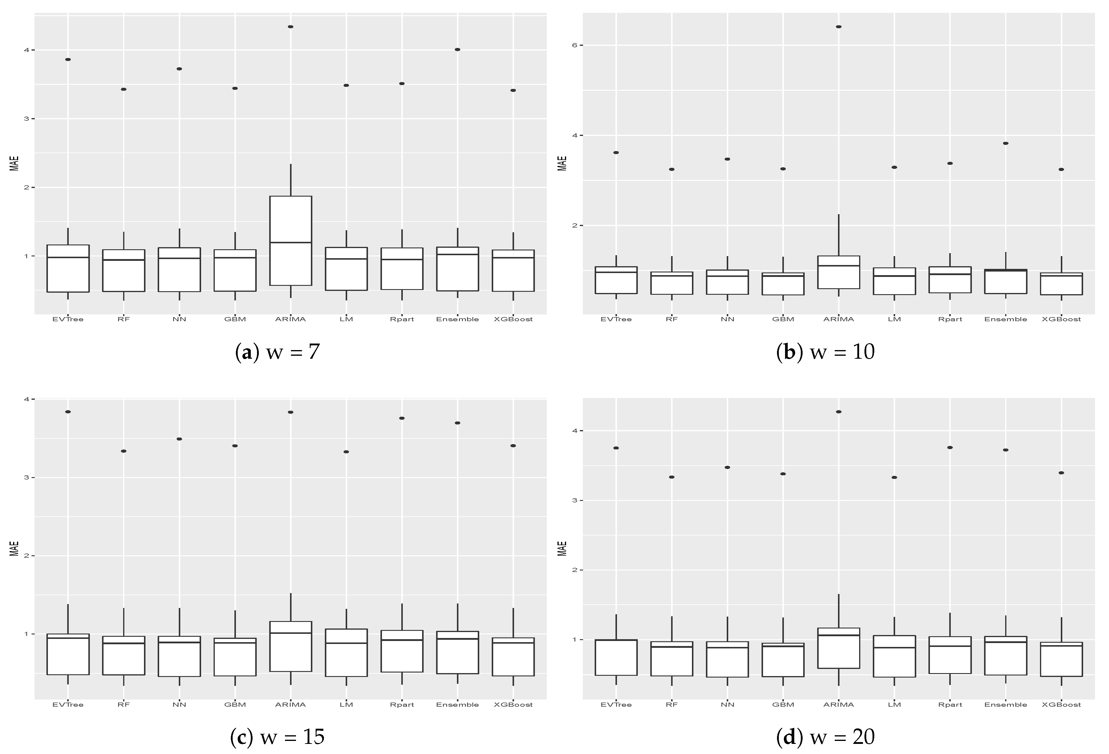
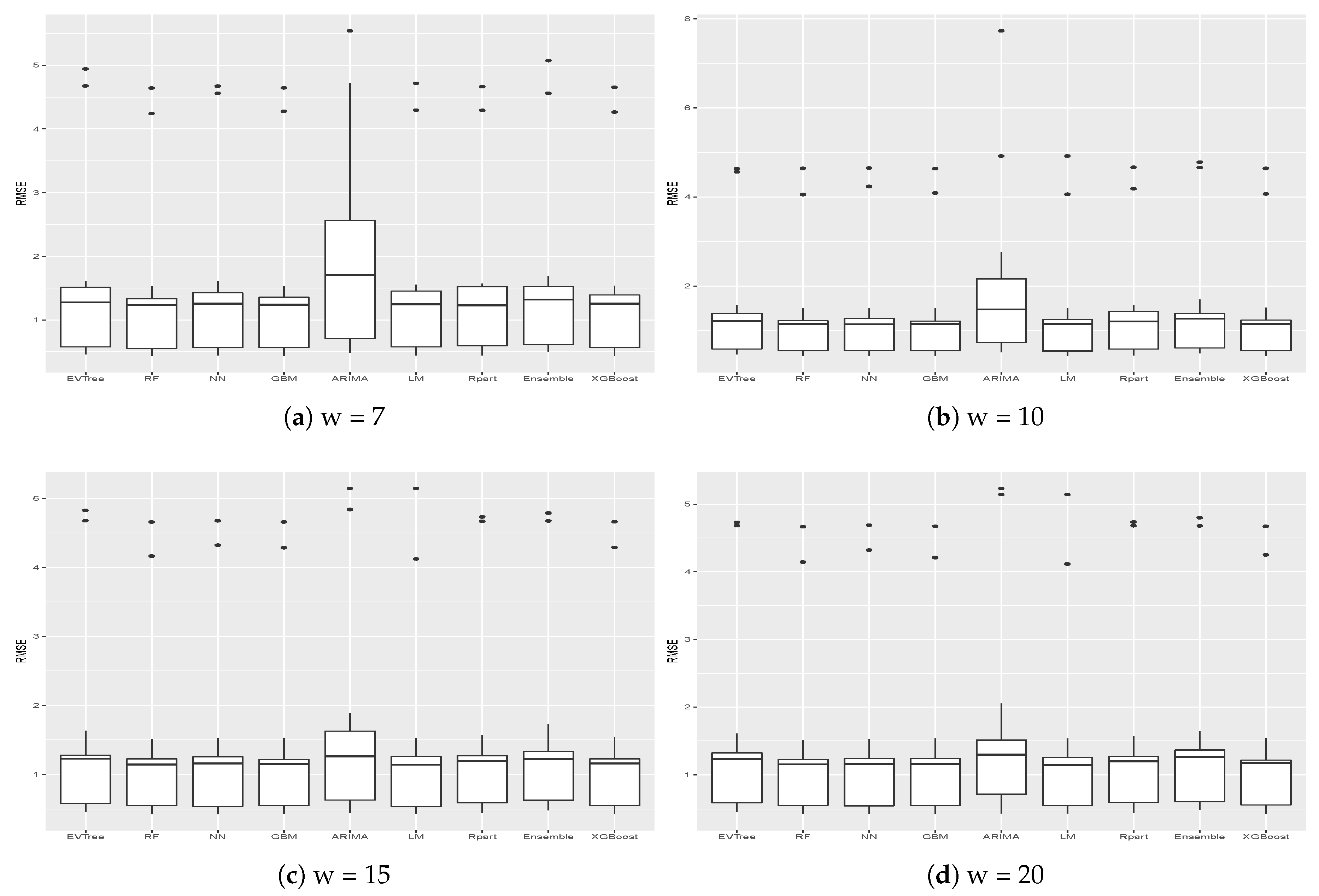
Figure 5 and Figure 6 show the results, in terms of MAE and RMSE, obtained by the different methods on all the buildings when different sizes of the historical window were used. By analyzing these results, we can conclude that, in general, the best size for the historical window to use is 10 days. In fact, with this value, the results obtained are generally better, in terms of both MAE and of RMSE. This is an important result, since it may help researchers to set the historical window for other time series forecasting regarding data generated by smart buildings, especially in the case where various days present missing values and cannot be considered for inducing a forecasting model. We can also see that ARIMA failed to produce good forecasts for the datasets used in this study. Another difference between ARIMA and the other methods is that, in general, the historical window of 10 days did not yield better results when used with this method. From the graphs, we can also notice the presence of outliers for both MAE and RMSE. Such values are relative to the results obtained on Building 25, where all methods used in this study achieved the worst prediction results. This was probably due to the characteristics of this building, which is different from the others, as it contains the university’s library. It is a newer building, whose surface is also much bigger than that of the other buildings. Moreover, the average energy consumption is significantly higher than the other buildings, as shown in Figure 2. Outliers relative to the RMSE were also due to the results obtained on Building 3, meaning that the predictions errors were larger on this building. In this case, the building is similar to the other ones considered, in terms of both features and for its usage and average energy consumption. This suggest that a further analysis conducted with the mangers of the buildings is needed for this case to acquire more insights.

In

Table 4. Average MAE obtained by the methods for all the values of historical window and on all the buildings. The standard deviation is shown in brackets.

Method	Average	Average for w = 10
RF	0.97 (0.75)	0.95 (0.75)
GBM	0.97 (0.76)	0.94 (0.75)
XGBoost	0.97 (0.76)	0.94 (0.75)
LM	0.98 (0.76)	0.96 (0.75)
NN	0.99 (0.81)	0.97 (0.81)
rpart	1.03 (0.75)	1.01 (0.79)
EVTree	1.04 (0.86)	1.02 (0.85)
ENSEMBLE	1.06 (0.87)	1.05 (0.90)
ARIMA	1.30 (1.15)	1.29 (1.14)
previous day	1.44 (1.18)	1.43 (1.22)
previous week	1.33 (1.12)	1.32 (1.14)

and

Table 5. Average RMSE obtained by the methods for all the values of historical window and on all the buildings.The standard deviation is shown in brackets.

Method	Average	Average for w = 10
RF	1.45 (1.32)	1.43 (1.35)
GBM	1.46 (1.33)	1.43 (1.35)
XGBoost	1.46 (1.33)	1.44 (1.35)
NN	1.47 (1.36)	1.45 (1.38)
LM	1.48 (1.39)	1.46 (1.40)
rpart	1.52 (1.37)	1.50 (1.36)
EVTree	1.56 (1.41)	1.54 (1.41)
ENSEMBLE	1.59 (1.42)	1.58 (1.45)
ARIMA	1.89 (1.67)	1.92 (1.85)
previous day	2.07 (1.90)	2.14 (1.99)
previous week	2.05 (1.91)	2.04 (1.96)

, we reported the average performances of the methods for all historical windows values and for all the buildings, and the average results obtained when a historical window of size 10 was used, since this value was considered to be the best one in the experimentation presented. Moreover, in the tables, we also report results obtained with two simple baseline benchmark forecasting models. In particular, we considered the energy consumption to be the same as the one of the previous day and of the previous week, i.e., of seven days earlier. Results obtained by these two methods are, as expected, not competitive if compared with the other methods. Results are ordered according to the averages results. In this way, we can obtain a sort of ranking of the methods, which is useful to establish the overall performances of the methods.

To assess the significance of the differences of the results obtained by the various techniques, we applied a two-tailed t-test with confidence level of 1%. The result of such test are summarized in

Table 6. Significance of the results regarding MAE according to two-tailed t-test with confidence level of 1%.

Method	EVTree	RF	NN	GBM	ARIMA	LM	rpart	ENSEMBLE	XGBoost
EVTree		s	s	s	s	s			s
RF					s		s	s
NN				s	s		s	s
GBM					s		s	s
ARIMA						s	s	s	s
LM							s	s
rpart									s
ENSEMBLE									s

and

Table 7. Significance of the results regarding RMSE according to two-tailed t-test with confidence level of 1%.

Method	EVTree	RF	NN	GBM	ARIMA	LM	rpart	ENSEMBLE	XGBoost
EVTree		s	s	s	s	s		s	s
RF			s		s		s	s	s
NN					s		s	s
GBM					s		s	s	s
ARIMA						s	s	s	s
LM								s
rpart								s	s
ENSEMBLE									s

, for the MAE and the RMSE, respectively. In these tables, a “s” means that the difference of results between two methods was considered to be significant. For example, in Table 6, we can notice that the average MAE obtained by RF was significantly better than the average MAE achieved by EVTree.

In the tables, we can see that all methods, but ARIMA, obtained better results when w was set to 10, which also confirmed the result regarding the optimal historical window size reported above. We can see that the first three strategies, i.e., RF, GBM and XGBoost, basically achieved the same results, even if, when the MAE was considered, GMB and XGBoost achieved slightly better results when w was set to 10.

In general, we can notice that, according to both MAE and RMSE, the best performing forecasting methods on the datasets used in this study were RF, GMB and XGBoost. Neural Networks and linear regression also obtained competitive results. It is interesting also to notice that the ensemble scheme proposed in [10] did not perform well on the datasets considered in this study, while the performances of the same methods were very competitive in a global short-term electric energy forecasting scenario. This could mean that a stacking ensemble approach, such as the one used in [10], is suitable for global energy consumption predictions, but that it is not suitable for a localized problem such as the one tackled in this study. ARIMA was confirmed to be the worst performing methods, suggesting that perhaps this method is not adequate for these kinds of problems.

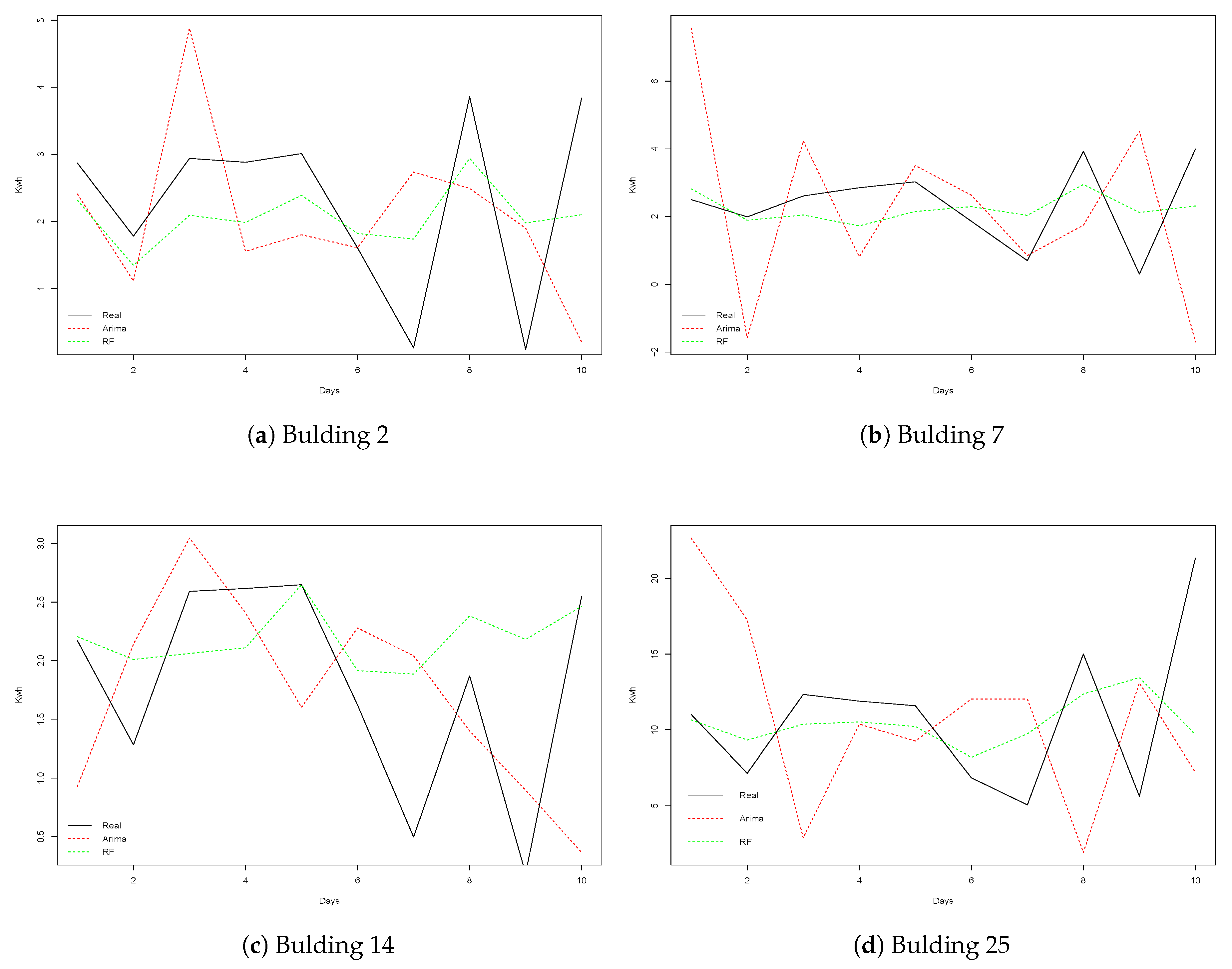
Finally, Figure 7 shows four examples of the observed and forecasted values from ARIMA and RF methods obtained on different buildings over a period of 10 days. Recall that RF is the method that achieved better results, while ARIMA is the worst performing technique. We can notice how RF better approximated the real values, while the errors made by ARIMA were in some cases significant. This fact caused ARIMA to perform poorly on the datasets used in this paper. From these graphs, we can conclude that the main difficulty of the datasets presented is to predict the energy consumption corresponding to the peaks represented in the graphs. However, methods such as RF can generally obtain predictions that are close to the observed values.

5. Conclusions and Future Work

In this paper, we have presented a comparative study of different time series forecasting techniques for predicting one-day electric energy consumption in non-residential buildings. In particular we were interested in both determining which strategy is more suitable for this kind of problem, and also to establish the optimal value for the historical window to be considered so as to produce the most accurate predictions. For such purpose, we compared nine forecasting methods on time series regarding data collected from thirteen smart buildings located in a university campus in Spain. The datasets used in this paper have never been used before, and are available on request. This represents an added value to the paper, since the datasets could represent a relevant resource for researches in this area.

From the experiments conducted, we can conclude that the best performing methods were Machine Learning based approaches. In particular, the Random Forests, Generalized Boosted Regression Mode and Extreme Gradient Boosting achieved, in general, the best performances on the data used in this work, since they achieved the lowest prediction errors. As such, they could represent the first choice for any further study on similar problems.

As far as the optimal historical window value is concerned, we found that, when the size of the window used was higher than seven, the results obtained improved. Moreover, the best results were achieved when the window size was set to 10, i.e., when ten days were considered to predict the electric energy consumption of the next day. This could help researchers facing similar forecasting scenarios.

As for future work, we are planning to apply a Deep Learning approach to the time series presented in this paper, since this strategy has obtained good results in other time series forecasting problems. A problem with this approach is represented by the setting of the parameters used to build the Deep Neural Network. In fact, a wrong setting can prevent such approach from obtaining good performances. To overcome this problem, we are also planning to use a Neurovolution approach [64,65,66]. In this approach, an Evolutionary Algorithm is used to establish a sub-optimal set of hyper parameters for the Deep Neural Network.

We are also planning to extend this study to other kinds of time series, for instance time series regarding the water and/or gas usage in smart buildings, and to include in the experimentation weather-related data. We also plan to to extend the experimentation to different buildings located in other regions to compare results obtained in different environmental conditions.