Dynamic Modeling of Wind Turbines Based on Estimated Wind Speed under Turbulent Conditions

Abstract

Large-scale wind turbines with a large blade radius rotates under fluctuating conditions depending on the blade position. The wind speed is maximum in the highest point when the blade in the upward position and minimum in the lowest point when the blade in the downward position. The spatial distribution of wind speed, which is known as the wind shear, leads to periodic fluctuations in the turbine rotor, which causes fluctuations in the generator output voltage and power. In addition, the turbine torque is affected by other factors such as tower shadow and turbine inertia. The space between the blade and tower, the tower diameter, and the blade diameter are very critical design factors that should be considered to reduce the output power fluctuations of a wind turbine generator. To model realistic characteristics while considering the critical factors of a wind turbine system, a wind turbine model is implemented using a squirrel-cage induction motor. Since the wind speed is the most important factor in modeling the aerodynamics of wind turbine, an accurate measurement or estimation is essential to have a valid model. This paper estimates the average wind speed, instead of measuring, from the generator power and rotating speed and models the turbine’s aerodynamics, including tower shadow and wind shear components, without having to measure the wind speed at any height. The proposed algorithm overcomes the errors of measuring wind speed in single or multiple locations by estimating the wind speed with estimation error less than 2%.

1. Introduction

Currently, electrical power is the main energy source in homes, industries, and workplaces. Industrial development and population growth have led to increased power consumption in the last three decades. Natural resources such as gas, petroleum, and coal are quickly depleting because of their growing use in power plants, vehicles, and industries. This serious problem motivates countries to find alternative energy sources through inexhaustible natural resources. One solution is found in clean, sustainable, inexhaustible, environmentally friendly, and renewable sources such as solar energy, wind energy, and tidal ocean currents. Wind energy has attracted more interest for several reasons and has increasingly become the most harvested renewable energy source [1]. Increased interest in wind turbines to generate electrical power entails studying and modeling the steady state and dynamic behavior of the wind turbine in laboratory conditions to prevent possible problems during installation and later use. In addition, over the last few decades, new control algorithms have been established to improve the performances of wind-generation systems. Before applying a new algorithm, it must be validated in the laboratory by simulating the entire system to verify the performance, control, and disturbances. Developing and improving the characteristics of a wind turbine simulator will help reach this objective and reflect the dynamic behavior of a wind turbine in a controlled environment [1,2,3].

Several wind turbine emulators have been proposed and studied in-depth. Some studies have investigated direct current (DC) motors to model the dynamic characteristics because of their robust characteristics such as output torque and input current using armature current control [4,5]. These emulators, however, entail a bulky and expensive DC motor, which requires frequent maintenance given its commutators and brushes. With regard to AC motor emulators, squirrel-cage induction motors (SCIM) are less costly and more reliable and robust [6]. Several research articles feature simple experiment platforms utilizing SCIM to model the characteristics of wind turbines. However, these emulators have simple wind turbine models that neglect the dynamics of wind turbine components, an important factor in wind energy systems [7,8]. A scaled-down emulator operated by a programmable wind speed model has been developed in several studies to investigate wind turbine performance during turbulences and stochastic wind speed changes [9].

Nevertheless, these emulators disregard several dynamic performance characteristics related to tower shadow, wind turbulence, and shear. These characteristics clearly influence the power quality and stability of wind-energy conversion systems (WECS) [10,11]. Specifically, fluctuations due to tower shadow and wind shear affect the WECS stability when the fluctuation frequency equals the natural frequency of the system [12]. In addition, all these studies used the measured wind speed, leading to inaccurate wind turbine dynamic characteristics and misleading results. Similarly, using anemometers in measuring wind speed leads to several problems in calibration and measurement accuracy and higher initial WECS costs. Therefore, using a wind speed estimator that is based on turbine characteristics instead of mechanical anemometers is desirable. In the literature, different techniques have been developed to estimate the effective wind speed without using an anemometer. These techniques can be categorized into two approaches. The first is the polynomial-based method for wind speed estimation, which uses a power equation as a function of the power coefficient and tip-speed ratio. This method utilizes root-finding algorithms to solve the polynomial with a high order of power coefficient for accurate estimation. However, the method is time-consuming and therefore impractical. Second, artificial intelligence and machine-learning methods, such as adaptive neuro-fuzzy inference systems [13,14], multilayer perceptron neural networks [15], and support vector regressions (SVR) [16,17], have been widely implemented to estimate effective wind speed. These methods help map the relation between electrical measured quantities, such as turbine power and rotational speed, and wind speed using numerous samples, and then use this online map to estimate the wind speed and the optimum wind speed, which produce the maximum turbine power point.

In this framework, a wind turbine modeling based on the estimated wind speed is presented by simulating both the static and dynamic characteristics using a SCIM. The tower shadow and wind shear are modeled as a function of the turbine parameters and continuously varying wind speed. A continuously varying wind speed profile composed of a sum of harmonics with wide-range frequencies to present the stochastic nature is developed. A particle swarm optimization–support vector regression (PSO-SVR) approach is employed for online wind speed estimation and generator speed adjustment for maximum power point tracking. Because the SVR performance alone severely depends on the tuning of its parameters, the PSO algorithm is used, which enables a fast online-based approach with high-parameter estimation accuracy. All dynamic features in the wind turbine are experimentally implemented to validate the proposed model shown in Figure 1.

2. Mathematical Model of Wind Energy System

Figure 1 illustrates the structure of the wind power generation system, which exploits a SCIM to emulate the wind turbine characteristics. The details of the wind emulator components, the DFG modeling, and the generator controller are discussed in the next sections.

2.1. Wind Turbine Model

The extracted power from the wind at any wind speed and turbine rotational speed is given by [18]

$$P_t=\frac{1}{2}\rho \pi R^2{\upsilon }^3{C}_p(\beta ,\lambda ).$$

(1)

Equation (1) indicates that the power coefficient is influenced by the TSR and the blade pitch angle, which is always below the rated wind speed. In wind energy systems, when the pitch angle is kept constant, the power captured will be a function only in the turbine rotational speed, maximum at a certain speed. Hence, to maximize the captured power, $\lambda$ should be kept at its optimum value ${\lambda }_{opt}$, and then the captured power is technically computed from the wind speed and the blade radius. When the wind speed is above the rated speed, the pitch angle adjusts to reduce the impact of excessive wind speed on the generated power. Here, β is kept constant for simplicity.

Figure 2 presents the turbine blade’s power variation with wind speed and rotational speed. The maximum power output occurs at a particular rotational speed.

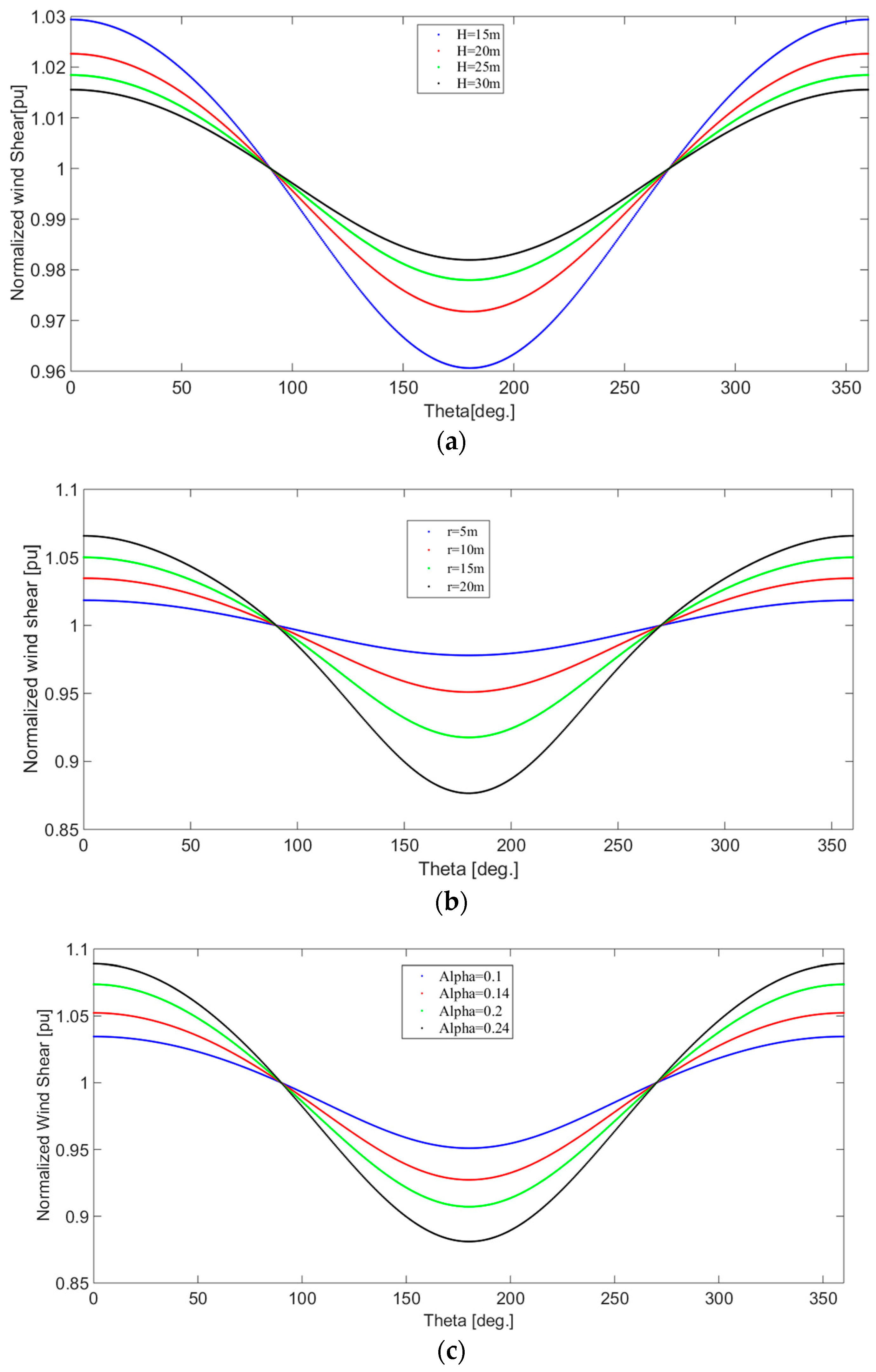
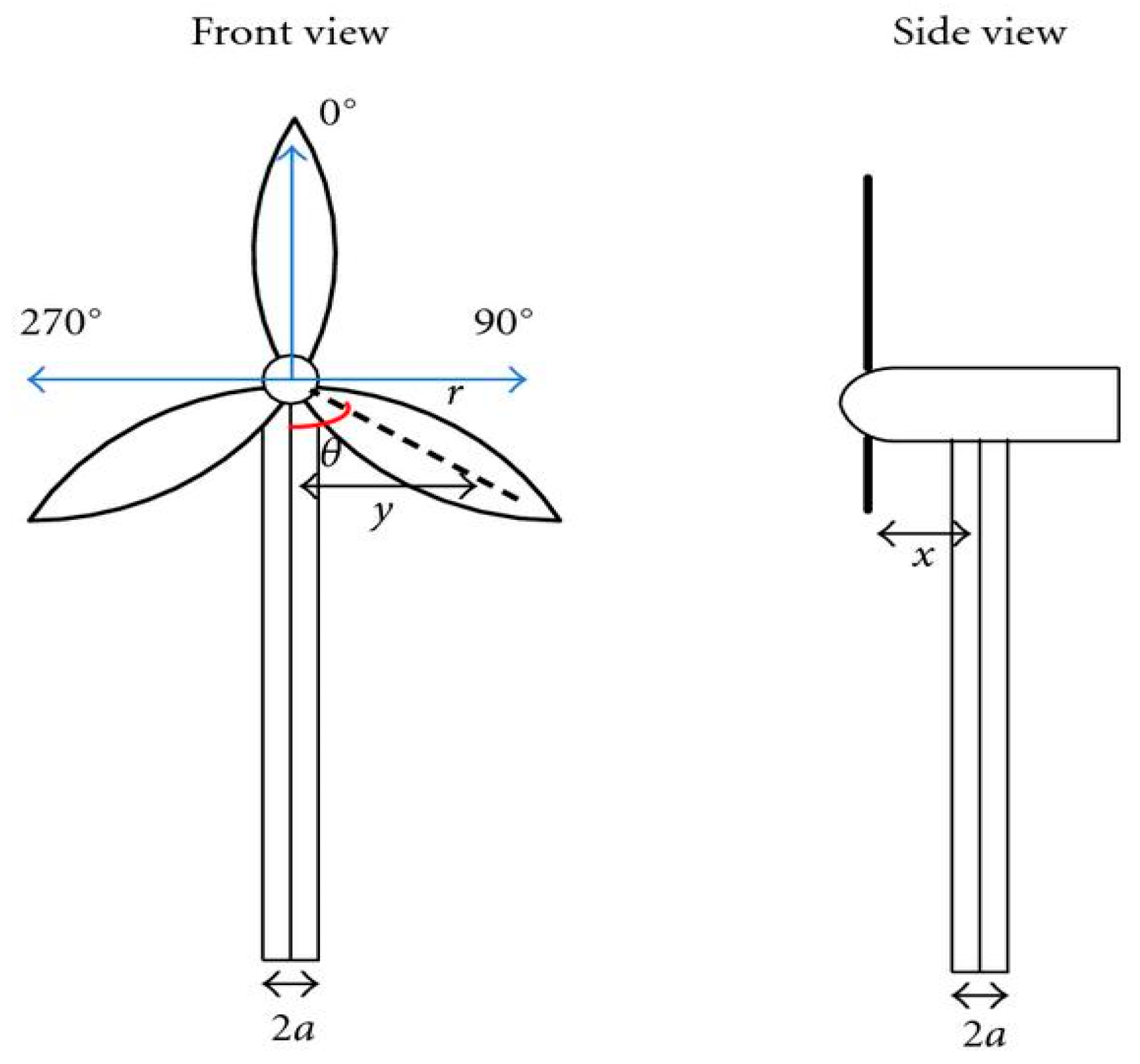
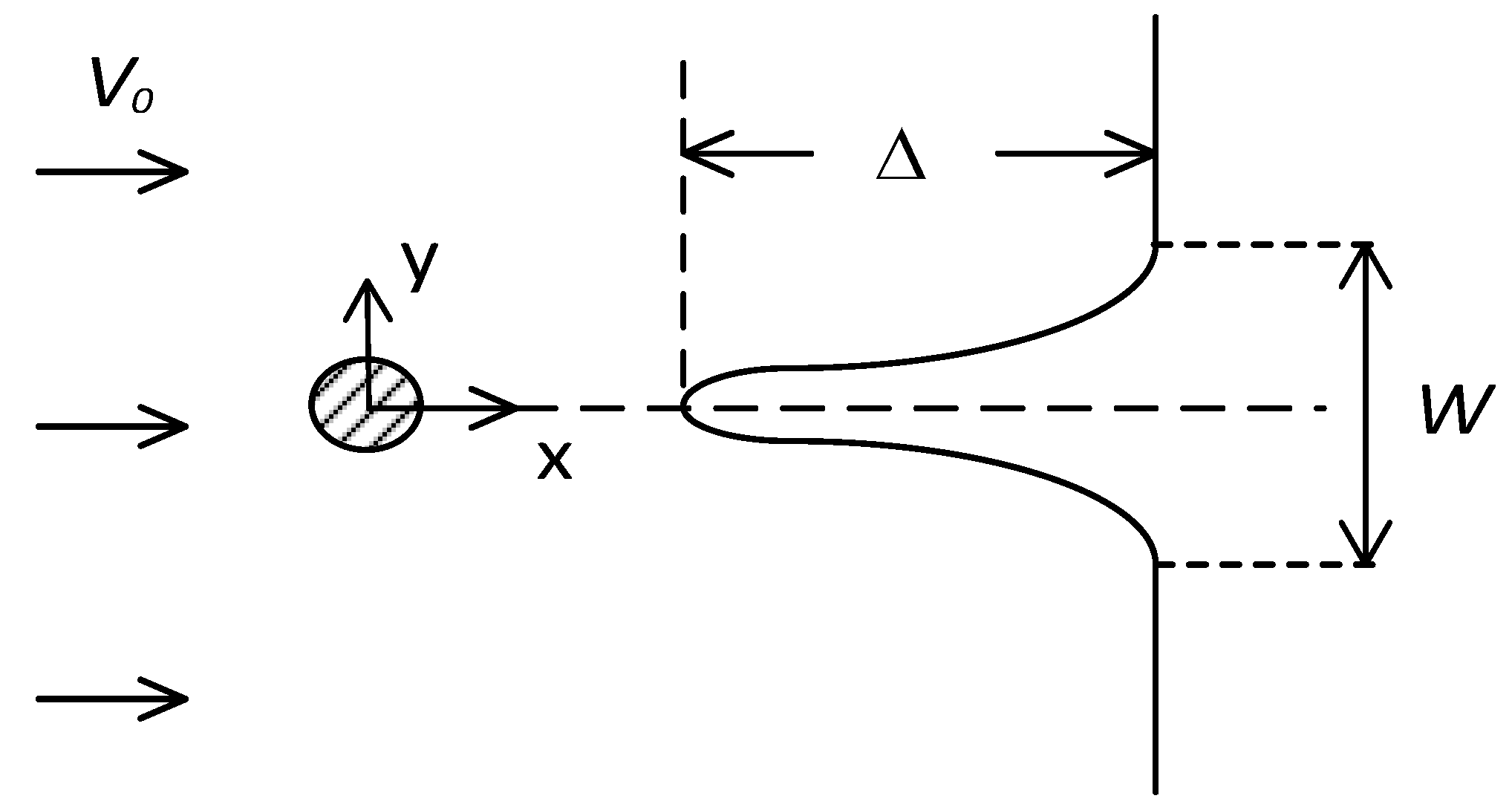
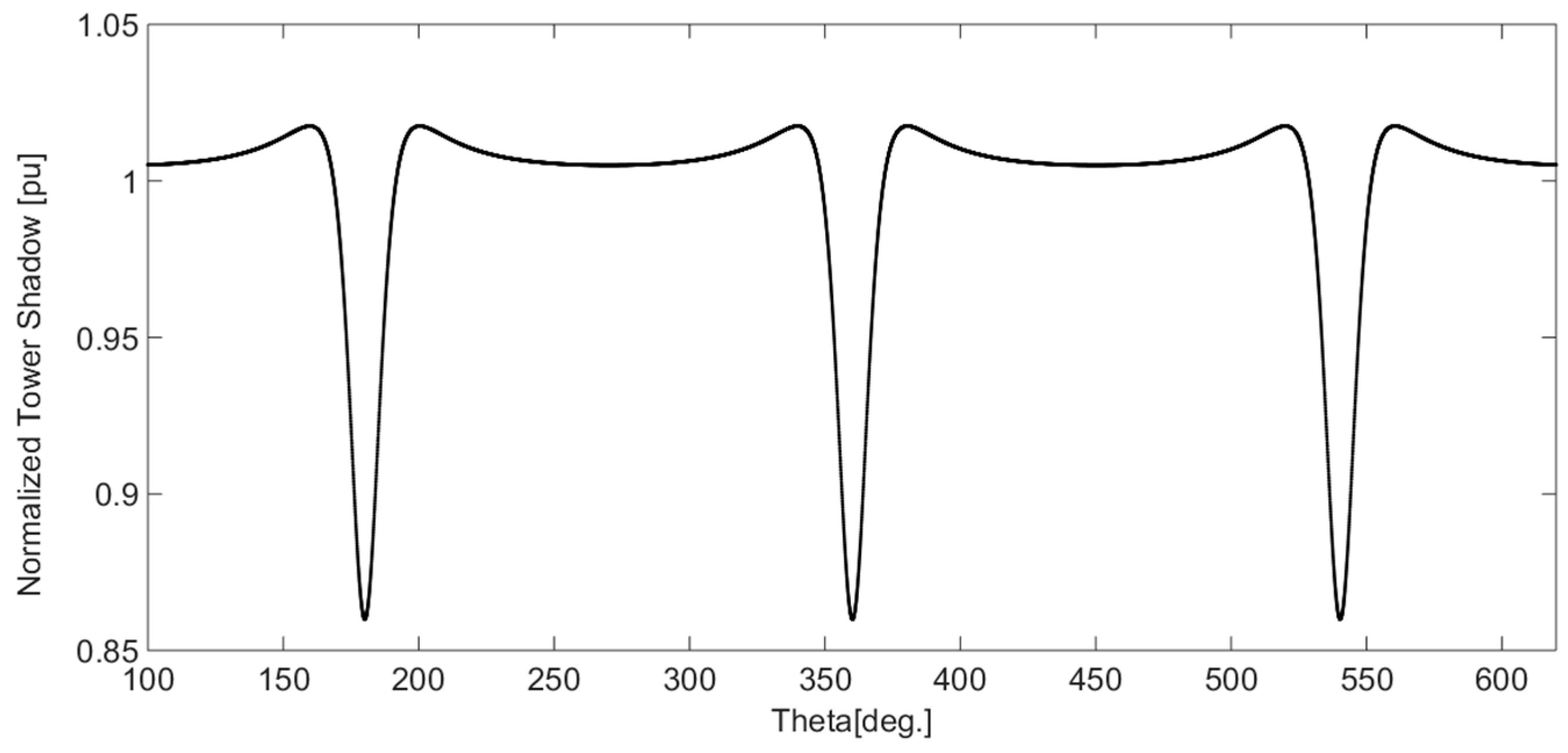
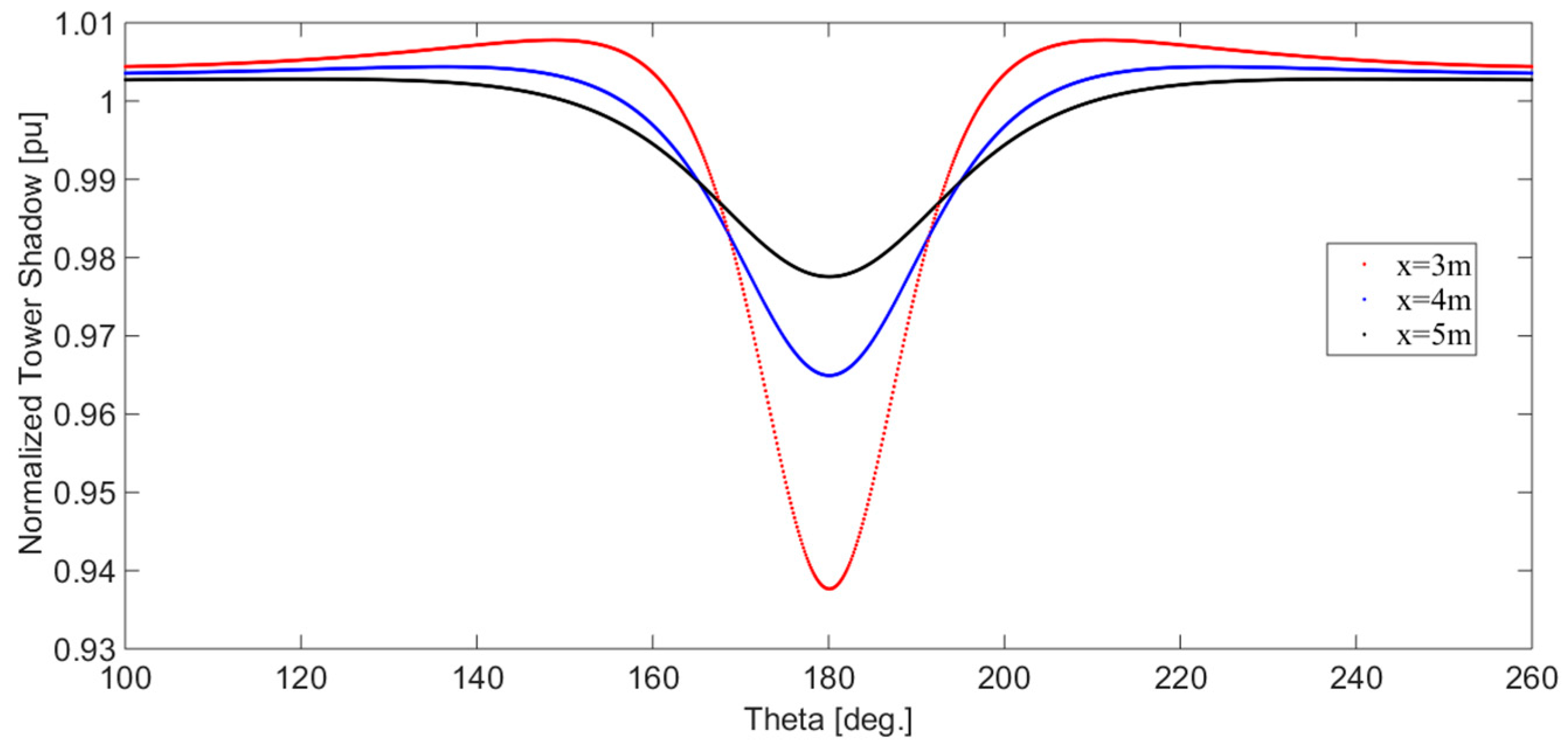
2.2. Wind Shear and Tower Shadow Model

Different wind speeds at different altitudes and the passing of the blade in front of the tower result in periodic torque pulsations in wind turbines.

Based on the height, the wind speed changes as follows [19,20]:

$$\frac{{\upsilon }_2}{{\upsilon }_1}={\left(\frac{h_2}{h_1}\right)}^{\alpha }.$$

(2)

Table 1. The empirical wind shear index [1].

Terrain	Empirical Wind Shear Exponent
Smooth, hard ground, lake, or ocean	0.1
Smooth, level, grass-covered	0.14
Tall row crops, low bushes with few trees	0.2
Many trees, occasional buildings	0.24

summarizes the geographical features and represents a general wind shear index [1].

As a result of height-dependent wind speeds, the turbine blades oscillate in response to the wind shear. Additionally, the amplitude of the wind speed increases with the height for different rotating angles from 0° to 360°. The wind speed in Equation (2) can be rewritten with respect to the speed at the turbine hub as follows [21]:

$$V(z)=V_h{\left(\frac{z}{H}\right)}^{\alpha }.$$

(3)

Considering the blade’s rotation and the unique wind shear at each angle, instead of expressing the wind shear in only the $z$ direction, the wind shear in Equation (6) can be expressed as a function of the blade rotational angle ${\psi }_b$ and radial distance $r$ from the rotor axis. The wind shear torque can be modeled as [22]:

$$V\left(r,{\psi }_b\right)=V_h{\left(\frac{r\cos {\psi }_b+H}{H}\right)}^{\alpha }$$

(4)

which can be written as

$$V\left(r,{\psi }_b\right)=V_h{\left(\frac{r\cos {\psi }_b+H}{H}\right)}^{\alpha }=V_h\left(\frac{r\cos {\psi }_b}{H}+1\right).$$

(5)

Equation (5) can be represented as a function of the wind shear disturbance $F\left(r,{\psi }_b\right)$:

$$V\left(r,{\psi }_b\right)=V_h\left(F\left(r,{\psi }_b\right)+1\right).$$

(6)

Due to wind shear, the wind speed can be expanded using Fourier transform as shown in the following Equation [22]:

$${\vartheta }_{ws}\left(r,{\psi }_b\right)=V_h\left[\begin{array}{l}\alpha \left(\frac{r}{H}\right)\cos {\psi }_b+\frac{\alpha (\alpha -1)}{2}{\left(\frac{r}{H}\right)}^2{\cos }^2{\psi }_b\\ +\frac{\alpha \left(\alpha -1\right)\left(\alpha -2\right)}{6}{\left(\frac{r}{H}\right)}^3{\cos }^3{\psi }_b\end{array}\right].$$

(7)

In low altitude, wind shear is influenced by the large amount of change in wind speed due to the friction of the surface. In addition, the longer the blade length of the wind turbine, the wider the turning radius of the rotor, and the larger the wind shear effect is. Figure 3 shows the wind shear effect of the turbine blade length, r hub height, and H empirical wind shear index as in Equation (7).

In the case of a large-diameter wind turbine, the blades experience a wide range of wind speeds in each revolution. With three-blade wind turbines, the frequent rotation through this wide range of speeds results in torque and power oscillations at three times the rotor rotational speed, called 3p frequency.

The tower radius (a), the distance of the blade origin from the tower midline (x), and the lateral distance of the blade from the tower midline (y) affect the tower shadow amplitude, as shown in Figure 4.

In front of the tower, the disturbance is nonnegligible and affects the wind speed and turbine output power. The wind speed reduces by a value of $\Delta$ in front of the tower and within the region W of 3–6 times of the tower diameter, as shown in Figure 5.

The tower shadow as a function of x and y is given by [23]

$$V\left(x,y\right)=V_h\left[1+\frac{a^2\left(x^2+y^2\right)}{{\left(x^2+y^2\right)}^2}\right]$$

(8)

$$V\left(x,y\right)=V_h+V_{tower}\left(x,y\right).$$

(9)

Expressing the tower shadow as a function of $r$ and ${\psi }_b$,

$$V_{tower}\left(r,{\psi }_b,x\right)=m\frac{a^2\left(r^2{\sin }^2{\psi }_b-x^2\right)}{{\left(r^2{\sin }^2{\psi }_b+x^2\right)}^2}$$

(10)

where $m=1+\frac{\alpha \left(\alpha -1\right)R^2}{8H^2}$.

Figure 6 shows wind shear and tower shadow effects at the tip of each blade at an average wind speed of 8 m/s. The tower shadow shape was calculated for different radial circulating points, from 8 m to 20 m in diameter, measured from the hub center, with an incremental distance of 8 m, as shown in Figure 6. When the diameter increases, the points on this circle perimeter experience short tower shadow intervals. The inner curve in Figure 6 indicates the circle with a diameter of 20 m, which has the lowest tower shadow interval. In contrast, the outer and widest curve in Figure 7 illustrates the shadow effect at a radius of 4 m. The parameters used in this test are $R=10 \mathrm{m},H=25 \mathrm{m},\alpha =0.15,a=0.75 \mathrm{m},$ and $x=3 \mathrm{m}.$

If the radial distance r is kept constant and the distance between the blade origin to the tower midline x varies from 3 m to 5 m, as Figure 8 illustrates, the tower shadow effect increases when the distance x is small. Therefore, the blades should be installed far from the tower to reduce the tower shadow effect. The tower shadow is given by

$$V_{ts}=\frac{m{V}_h}{3R^2}{\displaystyle \sum _{b=1}^3\left[\frac{a^2}{{\sin }^2{\psi }_b}\ln \left(\frac{R^2{\sin }^2{\psi }_b}{x^2}+1\right)-\frac{2a^2{R}^2}{R^2{\sin }^2{\psi }_b+x^2}\right]}.$$

(11)

For any wind speed value, the turbine torque T_t can be expressed as:

$$T_t=0.5\rho A{V}_h^3\frac{C_p(\lambda )}{{\omega }_r}.$$

(12)

The wind shear module implements the disturbance in torque due to wind shear given as

$$T_{ws}=\rho A{V}_h\frac{C_p(\lambda )}{\lambda }R{v}_{ws}$$

(13)

and the tower shadow module implements the disturbance in torque due to the tower shadow expressed as

$$T_{ts}=\rho A{V}_h\frac{C_p(\lambda )}{\lambda }R{v}_{ts}.$$

(14)

Due to turbine torque, wind shear, and tower shadow, the resultant aerodynamic torque is defined as Equation (15a).

However, the wind speed at the hub level is not accurate when modeling the turbine torques. Hence, a wind speed estimation method can be used to estimate the average wind speed to resemble real characteristics. The resultant torque in Equation (15a) can be expressed as Equation (15b):

$$T_{res}=0.5\rho A{V}_h^3\frac{C_p(\lambda )}{{\omega }_r}+\rho A{V}_h\frac{C_p(\lambda )}{\lambda }R\left(v_{ws}+v_{ts}\right).$$

(15a)

$$T_{res}=0.5\rho A{V}_o^3\frac{C_p(\lambda )}{{\omega }_r}+\rho A{V}_o\frac{C_p(\lambda )}{\lambda }R\left(v_{ws}+v_{ts}\right).$$

(15b)

2.3. Dynamic of the Rotating Masses in the Wind Turbine

The wind turbine rotor can be coupled directly to the generator shaft, or through a gearbox. The model traditionally used to represent the dynamic behavior of the wind group is the one that uses a system composed of two masses and their respective moments of inertia, with one mass representing the complete wind turbine and the other the generator rotor. These masses are connected by an axis that has its stiffness and damping modeled, as shown in Figure 9. A gearbox with an n ratio is used to couple the low-speed side of the turbine to the high-speed side of the generator.

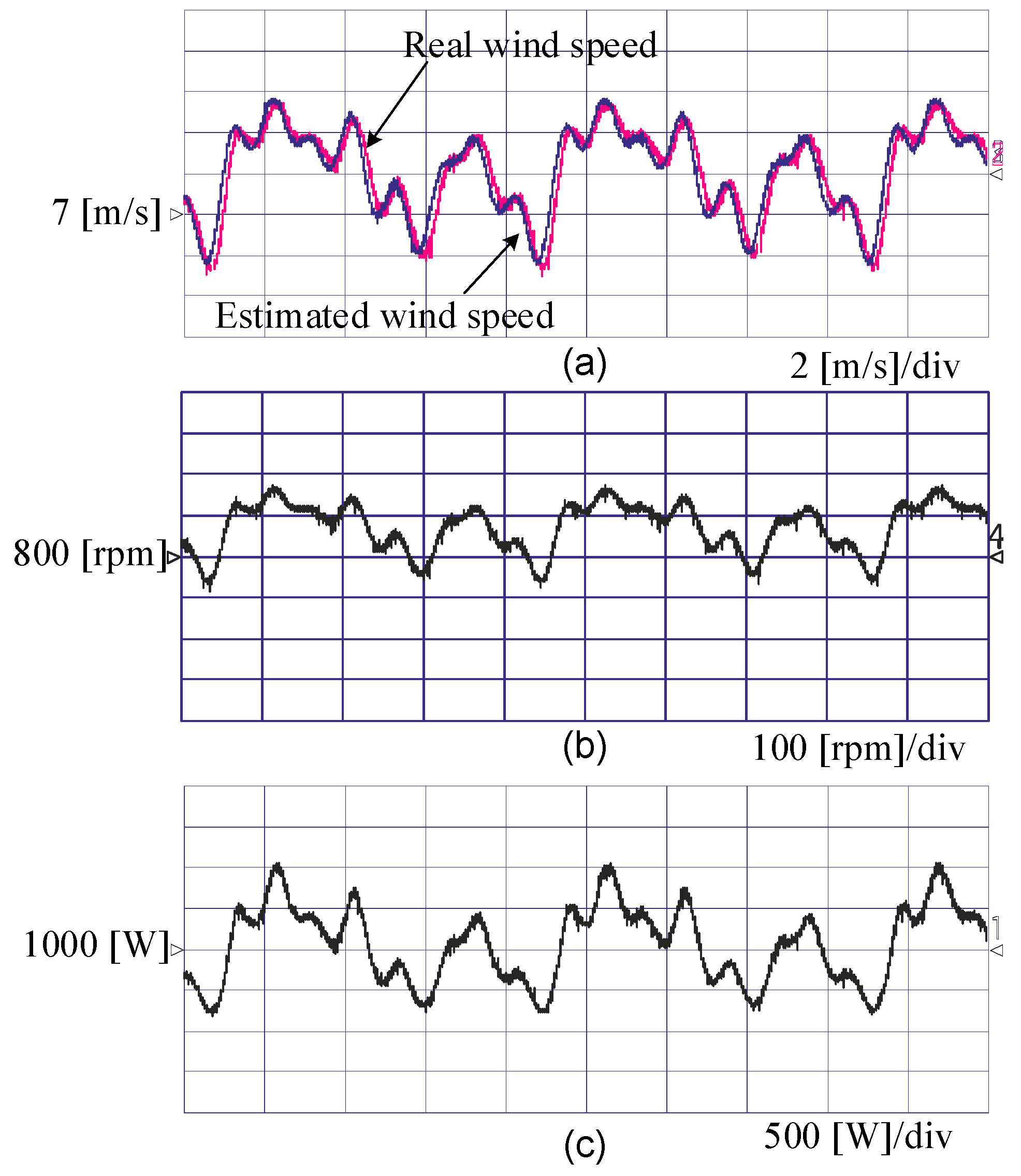
2.4. The Wind Speed Simulator

To model the torque fluctuation of a running wind turbine, a stochastic model for wind speed is required. This model is a sum of harmonics and is expressed as [24]

$$\upsilon (t)=V_o\left(1+{\displaystyle \sum _{i=1}^N{A}_i\sin ({\omega }_{i}t)}\right).$$

(16)

For each selected harmonic component, the amplitude can be written as a function of Dryden spectra ${\varphi }_u^{}$ as [25]

$$A_i=\frac{2}{\pi }\sqrt{\frac{1}{2}[{\phi }_u({\omega }_i)+{\phi }_u({\omega }_{i+1})]·[{\omega }_{i+1}-{\omega }_i]}$$

(17)

The longitudinal Dryden power spectrum is defined in terms of turbulence intensity $\sigma$, turbulence length, and harmonic frequency as follows [26]:

$${\varphi }_u(\omega )=\frac{L_u}{V_o}\frac{2{\sigma }^2}{\pi }\frac{1}{1+{(L_u\frac{\omega }{V_o})}^2}.$$

(18)

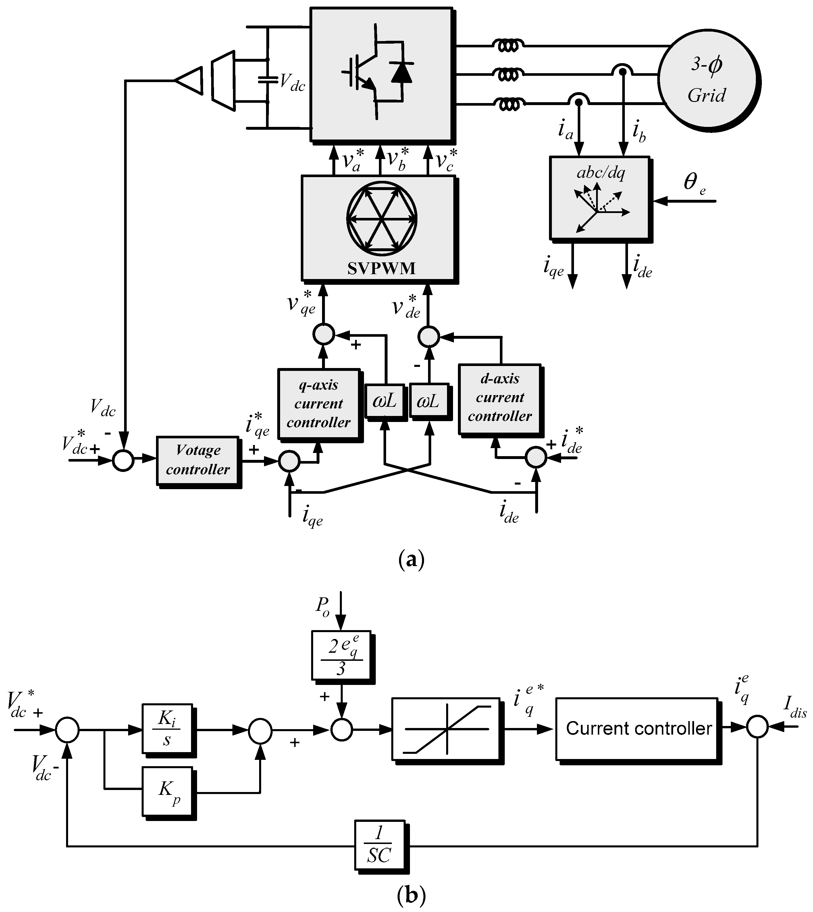
3. Induction Motor Control

The induction machine can be modeled by writing the dynamic equations in the d-q synchronous reference frame form as [27]

$$v_{ds}=i_{ds}{R}_s-{\omega }_e{\lambda }_{qs}+p{\lambda }_{ds}$$

(19)

$$v_{qs}=i_{qs}{R}_s+{\omega }_e{\lambda }_{ds}+p{\lambda }_{qs}$$

(20)

$$0=i_{dr}{R}_r+({\omega }_e-{\omega }_r){\lambda }_{qr}+p{\lambda }_{dr}$$

(21)

$$0=i_{qr}{R}_r+({\omega }_e-{\omega }_r){\lambda }_{dr}+p{\lambda }_{qr}.$$

(22)

The electromagnetic torque in the induction machine is fundamentally defined as

$$\begin{array}{ll}{T}_e& =\frac{3}{2}\frac{P}{2}{\lambda }_{dr}{i}_{qs}\\ & =K_{}{i}_{ds}{i}_{qs}=K_t{i}_{qs}.\end{array}$$

(23)

The motor torque and flux connected to the power source are controlled through the back-to-back converter. Whereas the motor flux is kept constant, the torque is controlled to provide the wind turbine characteristics. To generate a continuous variable torque, the torque current $i_{qs}$ is continuously controlled as defined in Equation (23). In experiment, the turbine reference torque and wind speed pattern are implemented by Equations (15b) and (16), respectively. The torque current reference $i_{qs}^{*}$ is then calculated from the torque equation by dividing it by the torque constant $K_t$, as shown in Figure 10a.

In fact, the motor reference d-axis current is kept constant at the value that maintains the minimum iron loss. In contrast, in the grid-side converter, the DC-link voltage is kept constant, and the output power factor is adjusted to unity by controlling the grid-side converter q-axis current and the d-axis current. The dc-link voltage is controlled to the desired value by using a proportional-integral (PI) controller and the change in the dc-link voltage represents a change in the q-axis current. A current feed-forward control loop is also used here to improve the dc-link voltage response to load disturbance. For unity power factor, the demand for the d-axis current is zero. Figure 10b shows a control block diagram of the grid-side converter.

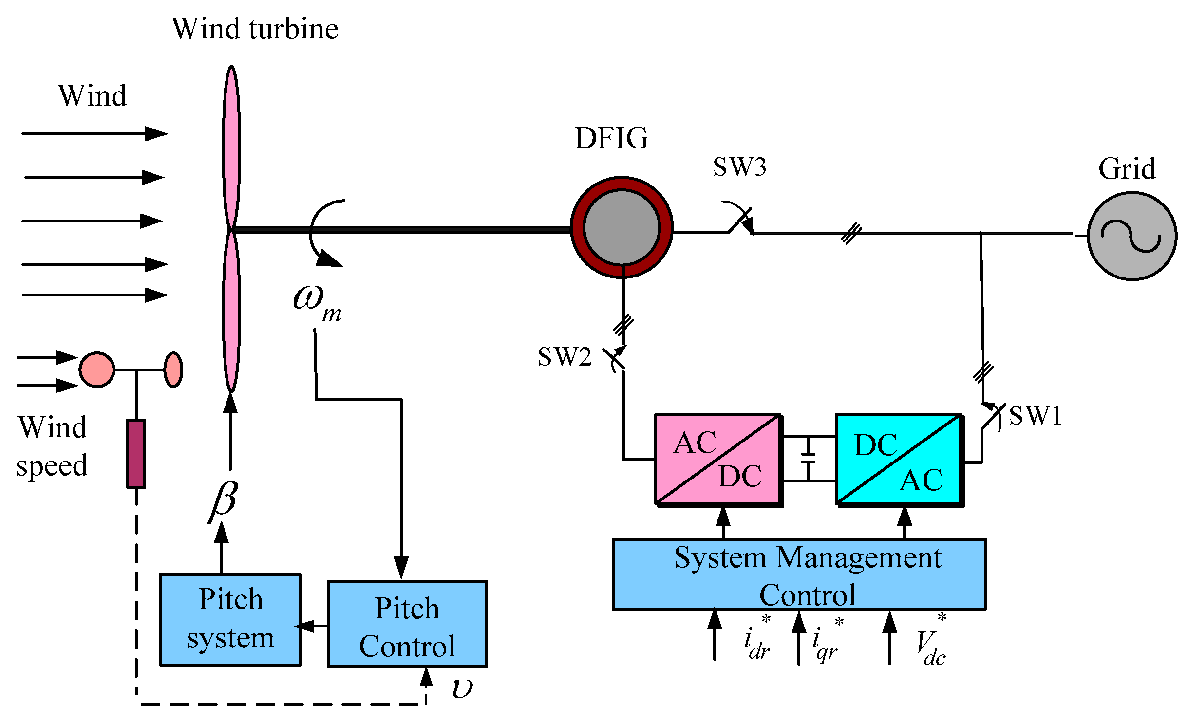
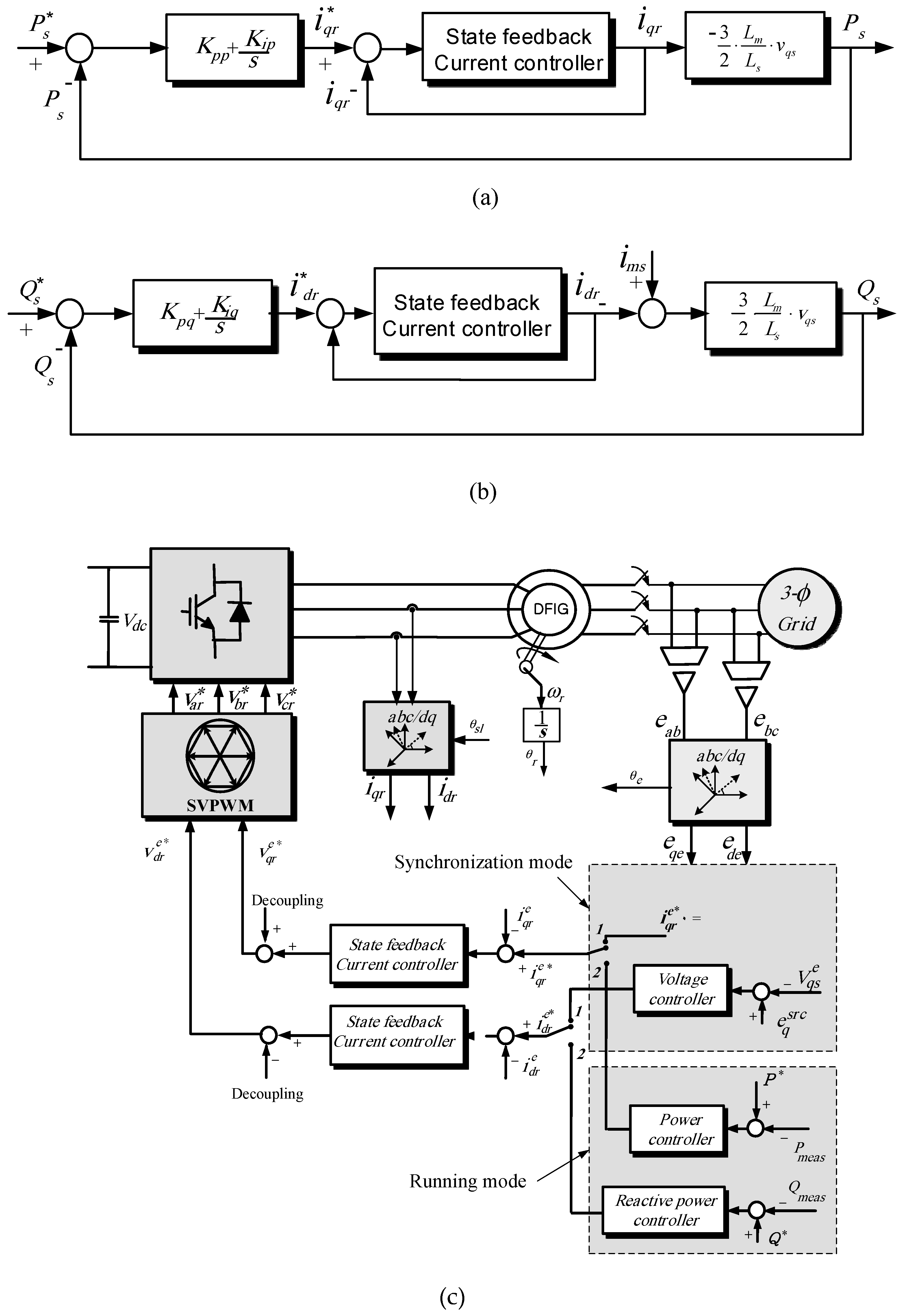
4. Control Scheme of DFIG

To control the active and reactive power in the stator side, a d-q reference frame synchronization with the stator flux is selected. The flux vector in the stator is aligned with the d-axis. The flux linkage of the rotor and stator is defined as [28]

$${\lambda }_s={\lambda }_{ds}=L_m{i}_{ms}=L_s{i}_{ds}+L_m{i}_{dr}$$

(24)

$${\lambda }_{dr}=\frac{L_m^2}{L_s}{i}_{ms}+\sigma L_r{i}_{dr}$$

(25)

$${\lambda }_{qr}=\sigma L_r{i}_{dr}$$

(26)

$$\sigma =1-\frac{L_m^2}{L_r{L}_s}.$$

(27)

Rotor voltages in the d-q reference frame can be written in terms of rotor and stator magnetizing currents.

$$v_{dr}=R_r{i}_{dr}+\sigma L_r\frac{d{i}_{dr}}{dt}-{\omega }_{sl}\sigma L_r{i}_{qr}$$

(28)

$$v_{qr}=R_r{i}_{qr}+\sigma L_r\frac{d{i}_{qr}}{dt}+{\omega }_{sl}(\sigma L_r{i}_{dr}+\frac{L_m^2}{L_s}{i}_{ms})$$

(29)

The stator flux angle is expressed as

$${\lambda }_{ds}^s={\displaystyle \int (v_{ds}^s-R_s{i}_{ds}^s)dt}$$

(30)

$${\lambda }_{qs}^s={\displaystyle \int (v_{qs}^s-R_s{i}_{qs}^s)dt}$$

(31)

$${\theta }_e={\tan }^{-1}\frac{{\lambda }_{qs}^s}{{\lambda }_{ds}^s}$$

(32)

where the superscript $s$ represents the parameters in the stationary reference frame.

Regulating the q-axis component of the rotor current controls either the active power of the DFIG stator side or the developed torque in the generator.

$$P_s=\frac{3}{2}(v_{qs}{i}_{qs}+v_{ds}{i}_{ds})=-\frac{3}{2}\cdot \frac{L_m}{L_s}\cdot v_{qs}{i}_{qr}$$

(33)

To directly control the stator-side reactive power, the rotor d-axis current component should be regulated. This reactive power can be expressed as

$$Q_s=\frac{3}{2}(v_{qs}{i}_{ds}-v_{ds}{i}_{qs})=\frac{3}{2}\cdot \frac{L_m}{L_s}\cdot v_{qs}(i_{ms}-i_{dr}).$$

(34)

The stator active and reactive powers are proportional to the current components $i_{qr}$, and $i_{dr}$, respectively.

The DFIG wind turbine system configuration consists of a DFIG connected to the utility grid through its stator. The back-to-back Pulse-Width Modulation (PWM) power converter enables a bidirectional power-flow control. As a result, the DFIG can operate either in sub-synchronous (${\omega }_r<{\omega }_e$) or in super-synchronous modes (${\omega }_r>{\omega }_e$). By calculating the stator active power, the control block diagram of the stator power is presented in the figure. The PI controller gains for the active and reactive power controllers are K_pp, K_ip, K_pq, and K_iq, respectively. The rotor reference q-axis current $i_{qr}^{*}$ is then calculated as the output of the active power controller and input for the inner current control loop. The rotor instantaneous q-axis current is then calculated from the sensed three-phase rotor currents and controlled to produce a reference q-axis rotor voltage. Normally, the output reactive power of the wind power conversion system is controlled as zero to keep unity power factor of the stator voltage and current. The stator reactive power is controlled to the desired value to produce the reference d-axis rotor voltage as shown in Figure 11b. One can see how the outer stator power feedback loop produces the rotor reference d-axis current $i_{dr}^{*}$ for the inner current feedback control loop. The reference q-axis rotor voltage is then produced by controlling the rotor d-axis component. The schematic diagram of the simplified control scheme is shown in Figure 11c.

The DFIG optimum power $P^{*}$ is the reference power value determined by the wind speed and rotor angular speed of the power controller loop. A simple proportional-integral (PI) controller can be utilized to regulate the d-q component of the rotor current only if the reference frames for both the measured and reference current vectors match [29].

To achieve the full control of the grid-side current, the dc-link voltage must be boosted to a level higher than the amplitude of the line-line voltage. The power flow of the grid-side converter is controlled so as to keep the dc-link voltage constant. To maintain the dc-link voltage constant and to ensure the reactive power flowing into the grid at null, the grid-side converter currents are controlled using the d-q vector control approach. The dc-link voltage is controlled to the desired value by using an IP controller and the change in the dc-link voltage represents a change in the q-axis current. A simple voltage control scheme is shown in Figure 12a. A current feed-forward control loop is also used here to improve the dc-link voltage response to load disturbance. For unity power factor, the demand for the d-axis current is zero. Figure 12b shows a control block diagram of the grid-side converter.

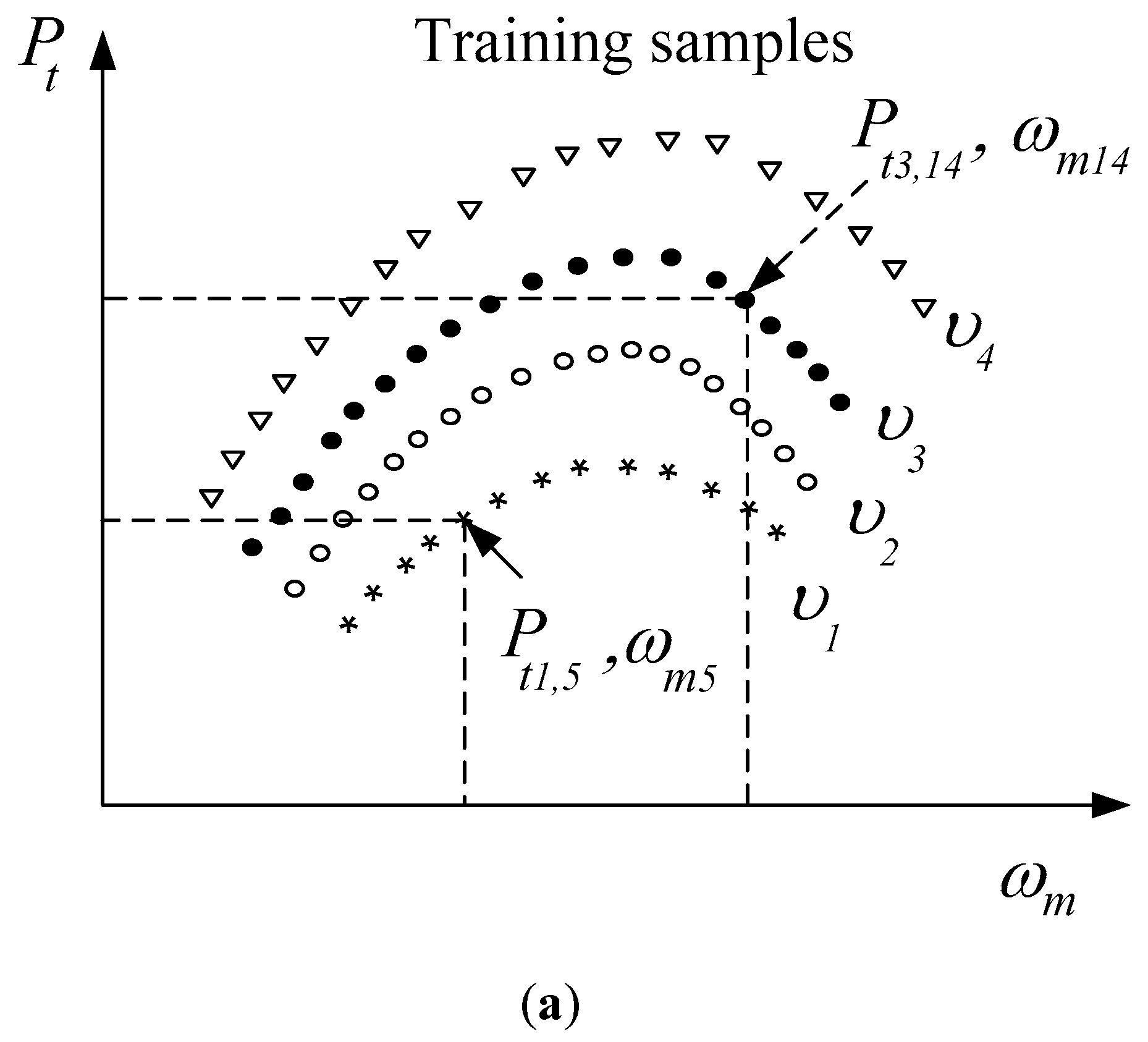
5. Wind Speed Estimation

5.1. Support Vector Regression

The SVR is an algorithm that estimates a function that predicts unknown mapping between a system’s l-dimensional inputs and real output using a series of training data. When the map is accurately constructed, the relation between the inputs and output is then used to predict the target output. The regression algorithm approximates the unknown desired function in the following form [30]:

$$f(x)=(w.\mathsf{\Phi }(x))+b.$$

(35)

These values are extracted from the available training data to determine the target function. The first step is to obtain both $w$ and $b$ to minimize the real data differences outside the $\epsilon$-insensitive region, which are determined by slack variables $\xi$ and ${\xi }^{*}$. To minimize the empirical risk, the slack variables are applied as [31]

$$R_{reg}\left(f\right)=\frac{1}{2}{\Vert w\Vert }^2+C{\displaystyle \sum _{i=1}^n\mathsf{\Gamma }\left(f(x_i)-y_i\right)}$$

(36)

subject to

$$\begin{array}{l}{y}_i-w.\mathsf{\Phi }(x_i)-b\le \epsilon +{\xi }_i^{*}\\ w.\mathsf{\Phi }(x_i)+b-y_i\le \epsilon +{\xi }_i\end{array}$$

(37)

$$i=1,2,\dots \dots \dots \dots n {\xi }_i,{\xi }_i^{*}\ge 0.$$

The penalty factor $C$ determines the compromise value between reduction to minimize both empirical and global errors and the model complexity term ${\Vert w\Vert }^2$. SVR reduces the error to zero if the penalty factor is very high. This option leads to a complex model. However, a low $C$ leads to high estimation errors.

The regression problem in Equation (24) is then solved using dual multipliers:

$$f(x)={\displaystyle \sum _{i=1}^n({\alpha }_i-{\alpha }_i^{*}).K}(x_i,x)+b$$

(38)

where $K(x_i,x_j)=\mathsf{\Phi }{(x_i)}^T\mathsf{\Phi }(x_j)$ is the kernel function that enables a dot product in high-dimensional feature space using low-dimensional space data input without calculating the function. The radial base function that is used in the framework is expressed as shown in the following equation:

$$K(x_i,x)=\exp \{-\frac{{\left|x_i-x\right|}^2}{{\sigma }^2}\}.$$

(39)

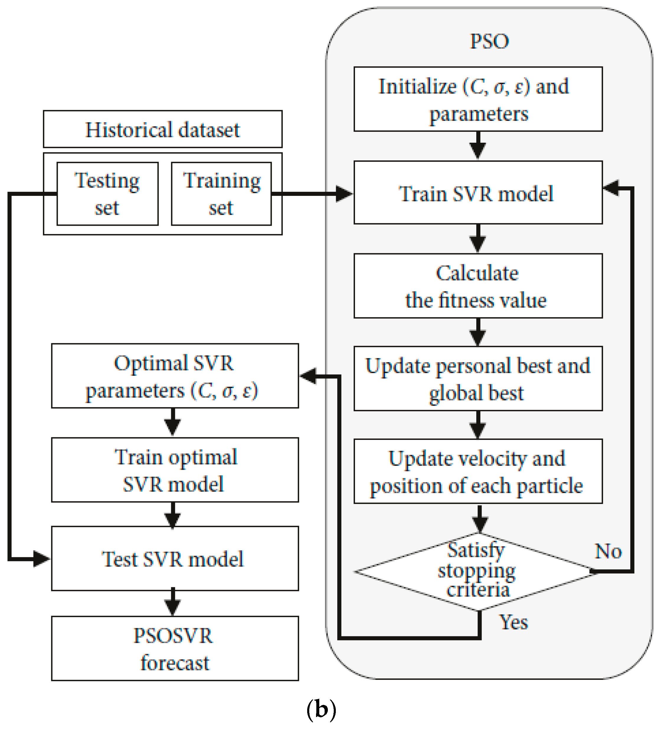
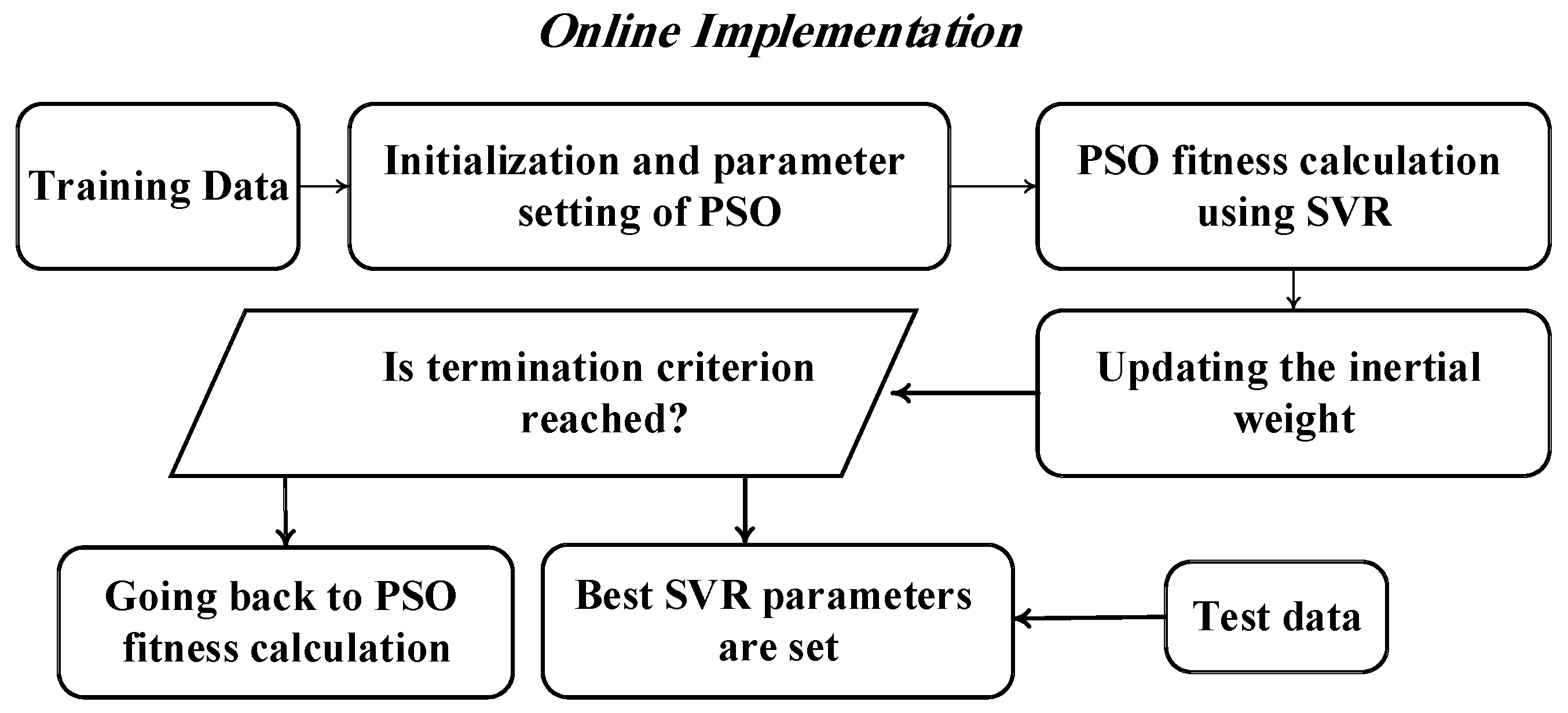
5.2. Particle Swarm Optimization

The PSO method is a population-based search technique that starts with a population of random solutions called particles [32]. Every solution within the swarm is called a particle [33]. The swarm is arbitrarily initialized and updated in each reiteration t to fully adapt the fitness function. The $i^{th}$ d-dimensional particle is characterized by its location vector $P_i^t=$ $P_{i1}^t$, $P_{i2}^t$, $\dots ,$ $P_{id}^t$ and its speed vector $v_i^t=$ $v_{i1}^t$, $v_{i2}^t$, $\dots ,$ $v_{id}^t$. Each particle knows its best personal location $P_{i,Best}^t$ and the entire population’s best global solution $G_{Best}^t$. The position of the population at iteration t is $P_{}^t=$ $P_1^t$, $P_2^t$, $,\dots ,$ $P_N^t$, where $N$ is the population size. Each particle updates its location according to Equations (40) and (42):

$$v_i^{t+1}=w^t{v}_i^t+c_1{r}_1(p_{i,Best}^t-p_i^t)+c_2{r}_2(p_{i,Best}^t-p_i^t)$$

(40)

$$p_i^{t+1}=p_i^t+v_i^{t+1},i=1,2,3,\dots ,N.$$

(41)

The constriction coefficients introduced in [33,34] are used to set $c_1$ and $c_2$:

$$x=\frac{2}{\varphi -1+\sqrt{{\varphi }^2-4\varphi }}$$

(42)

$$c_1=x{\varphi }_1, c_2=x{\varphi }_2$$

(43)

where $\varphi ={\varphi }_1+{\varphi }_2>4$. In this paper, ${\varphi }_1={\varphi }_2=2.05$; thus,$c_1=c_2=1.4962$. Location and speed boundaries are adjusted such that if a particle tries to pass the allowable boundaries, a limiting procedure brings it back within the permissible limit. If the best personal solution $P_{Best}^{i,t}$ has a higher fitness than the current best global solution $G_{Best}^{t-1}$, then $G_{Best}^t$ is equal to $P_{Best}^{i,t}$ [35]. The end points are determined when the best global solution results in a permissible fitness or when a predetermined number of iterations is achieved.

The wind speed estimation using PSO-SVR method can be described in steps as follows:

• Enter original data for estimation, known as the data preparation step;
• Initialize the particles with random velocities and positions, known as particles optimization;
• Perform an offline training process for SVR with training samples assessing each particle fitness value of the PSO for the SVR;
• Update each particle velocity and position until the termination condition is satisfied;
• Construct and retrain the SVR estimation model based on the optimal parameters.

Training data are obtained from the turbine power equation with pre-specified rotor speed and wind velocity samples. During on-line operation, the turbine power is calculated as

$$P_t=J{\omega }_m\frac{d{\omega }_m}{dt}+P_g.$$

(44)

For each sample, the rotor speed and the corresponding turbine power (${\omega }_i,p_{i,j}|i=1,\dots 50,j=1,\dots 50$) are combined as a pair for the inputs of SVR estimator as shown in Figure 13a. For any operating condition, if the turbine power and the rotor speed are known, the wind speed can be calculated as described in the framework of a PSO-SVR method in Figure 13b [36].

The detailed implementation process of the proposed method is shown in Figure 14.

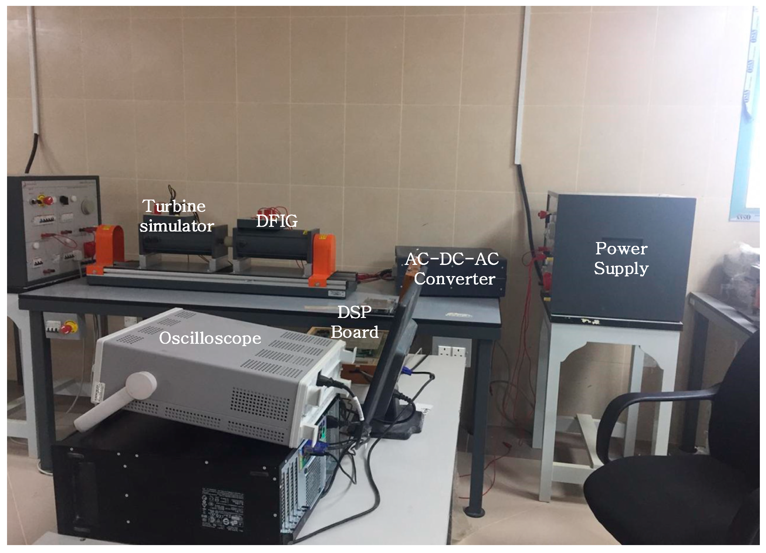
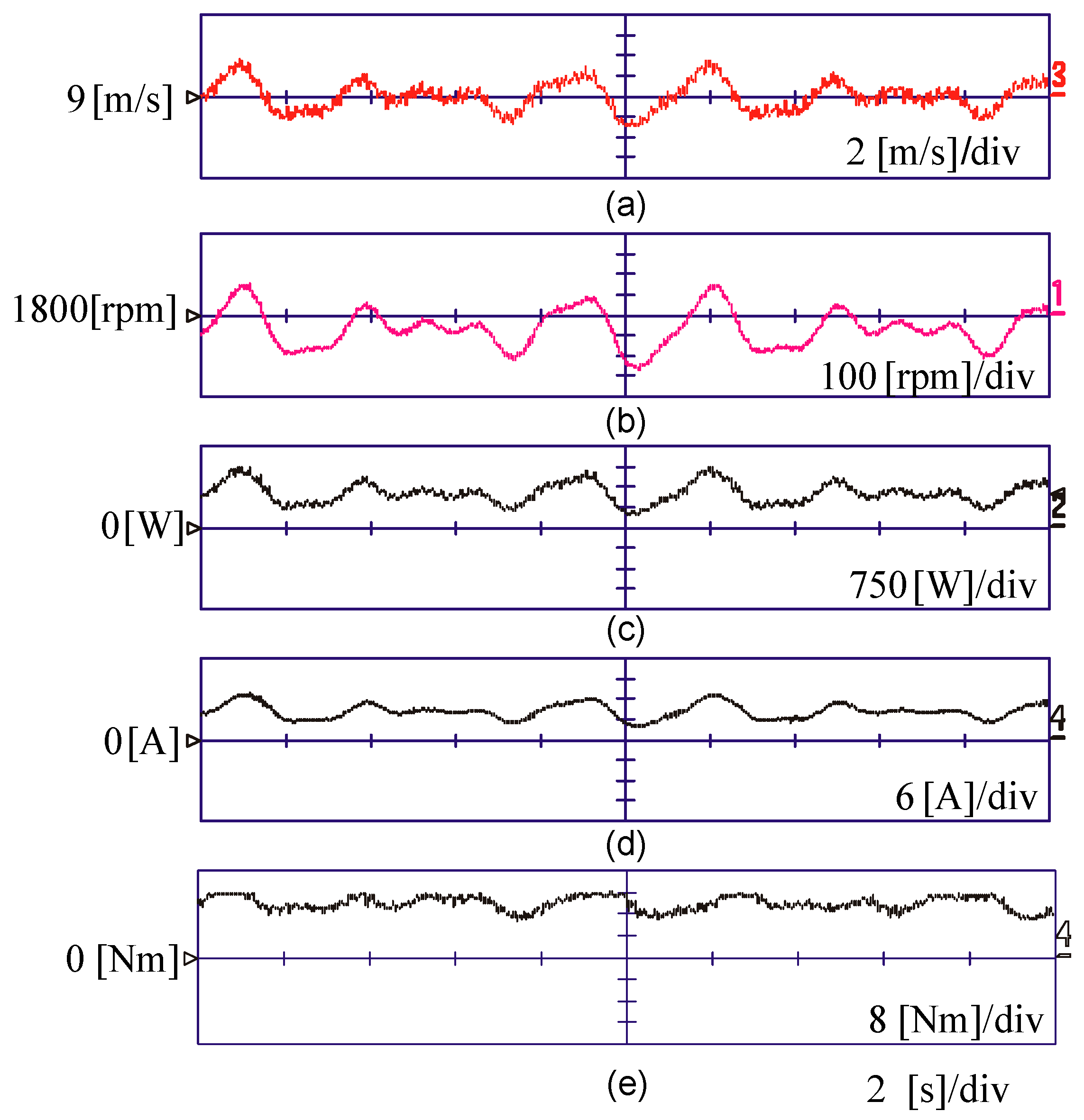
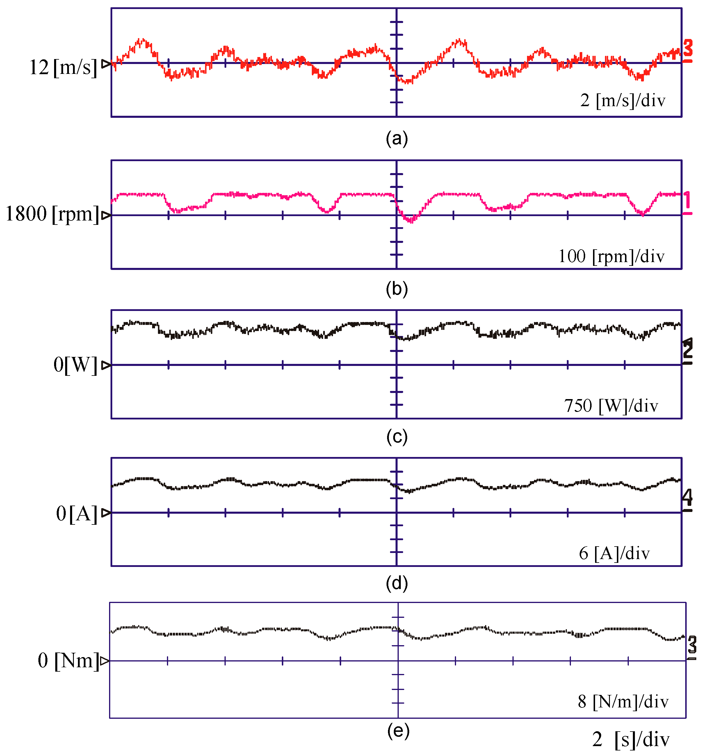
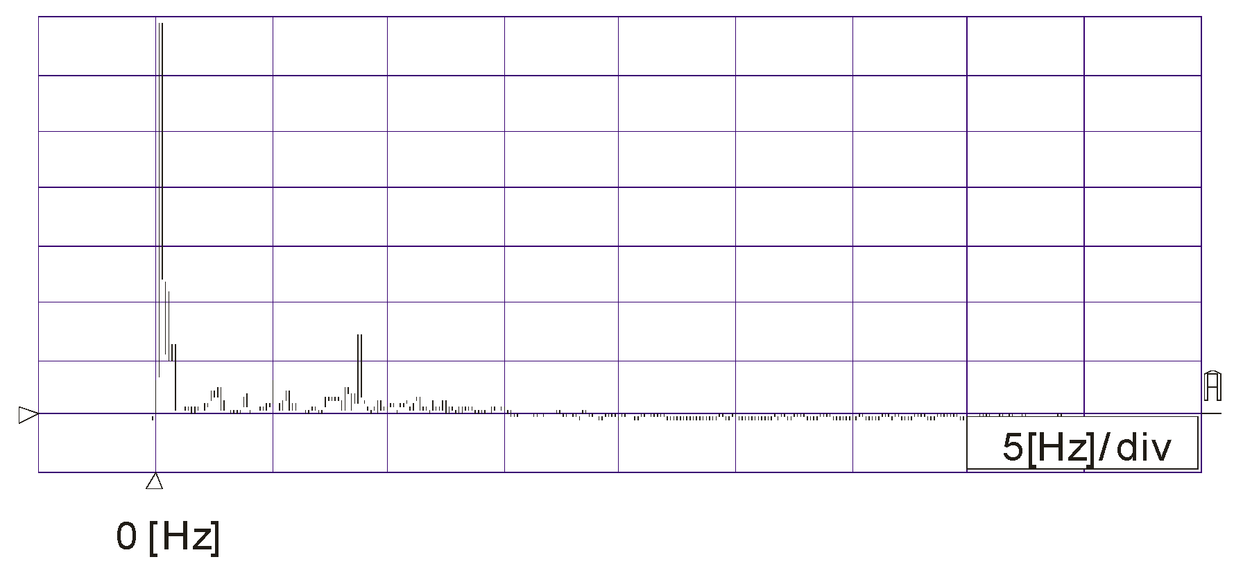
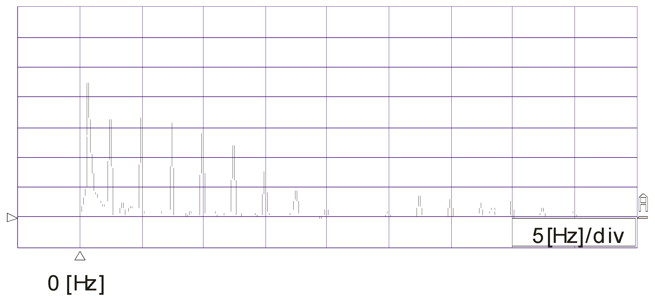
6. Experimental Results

It is desirable that the wind turbine simulator is implemented in hardware (M-G set) to test the WECS operation in the laboratory. The hardware setup consists of the DFIG-driven by the SCIM, PWM converters, and digital signal processor (DSP) control boards as shown in Figure 15. The specifications of the wind turbine blade modeled for the simulator, the SCIM motor ratings and parameters, and the experimental setup are listed in

Table A1. Parameters of turbine blade model.

Parameters	Value
Blade radius	0.95 m
Max. power conv. coeff.	0.45
Optimal tip-speed ratio	7
Cut-in speed	4 m/s
Rated wind speed	13 m/s

and

Table A2. Parameters of 3kW SCIG.

Parameters	Value
Stator resistance	0.93 Ω
Rotor resistance	0.533 Ω
Iron loss resistance	190 Ω
Stator leakage inductance	0.003 H
Rotor leakage inductance	0.003 H
Mutual inductance	0.076 H

in the Appendix A. Figure 16 shows the turbine performance for turbulent wind speed, of which the spectrum is similar to the real wind speed pattern. High estimation accuracy and very high PSO-SVR dynamic performance is illustrated in Figure 16a. It is noticeable that the estimated wind speed has a slight difference from the real value due to the trade-off between the minimizing error and the model complexity. The generator rotational speed follows the wind speed pattern in all wind speed values, as shown in Figure 16b. Figure 16c plots the generator output power versus variable wind speed.

By adding the effect of wind shear and tower shadow, the total turbine torque oscillates in the same frequency. However, the inertia of the turbine leads to the reduction of the effect of both disturbances as presented in Figure 17a,b.

It can be observed that periodic components are concentrated on frequency multiples of the blade passing frequency, mainly 3p, 6p … etc., as it is shown in Figure 18. It should be expected that the amplitude decreases when they increase in order.

Equation (16) is then used to generate a stochastic model of the wind speed to model the real nature of instantaneous wind speed, as shown in Figure 19a. The turbulent wind speed spectrum is generated by the wind speed simulator. The parameters are chosen as follows: $V_o=9 [m/s],N=15$ in (11), $L=90 [m]$ and $\sigma =0.2$ in Equation (13). It is obvious that the tower shadow and the wind shear are quite significant for the variations of the turbine torque and power. The range of harmonic content in the wind speed profile is from 0.1 Hz to 10 Hz. From Figure 19, it can be observed that the turbine performance for turbulent wind speed continuously follows the wind speed pattern, as shown in Figure 19b–e. During this low wind speed, the pitch angle controller keeps the pitch angle position in the minimum value, which is zero. However, when the average wind speed increases to 12 m/s, the generator rotational speed and generator output power increase to the maximum limits, which activate the pitch angle controller to increase the pitch angle to the predetermined position based on the wind speed value. In this case, the generator output power and the generator rotating speed are constant and equal to the rated values. Figure 20 depicts the transition between the maximum power point tracking (MPPT) mode and constant power mode. The generator output power is constant when the speed goes higher than 13 m/s in Figure 20a, as shown in Figure 20c. The generator speed, rotor q-axis current, torque and have the same trend as in Figure 20b, d and e, respectively.

The wind variation is modeled as a sum of wide range harmonics with frequencies 0.1–10 Hz. The spectrum of the turbulent wind speed in Figure 21 shows the low frequency components of the wind speed. The measured stator and rotor currents are shown in Figure 22a,b. From the stator current, it is obvious that the currents are almost sinusoidal.

The operating modes of a wind turbine are obtained, as in Figure 23. This curve is divided into four regions, as follows:

-

Region AB, when the wind speed is less than the cut-in speed when the rotational speed is less than the minimum rotational speed for optimum operation.

-

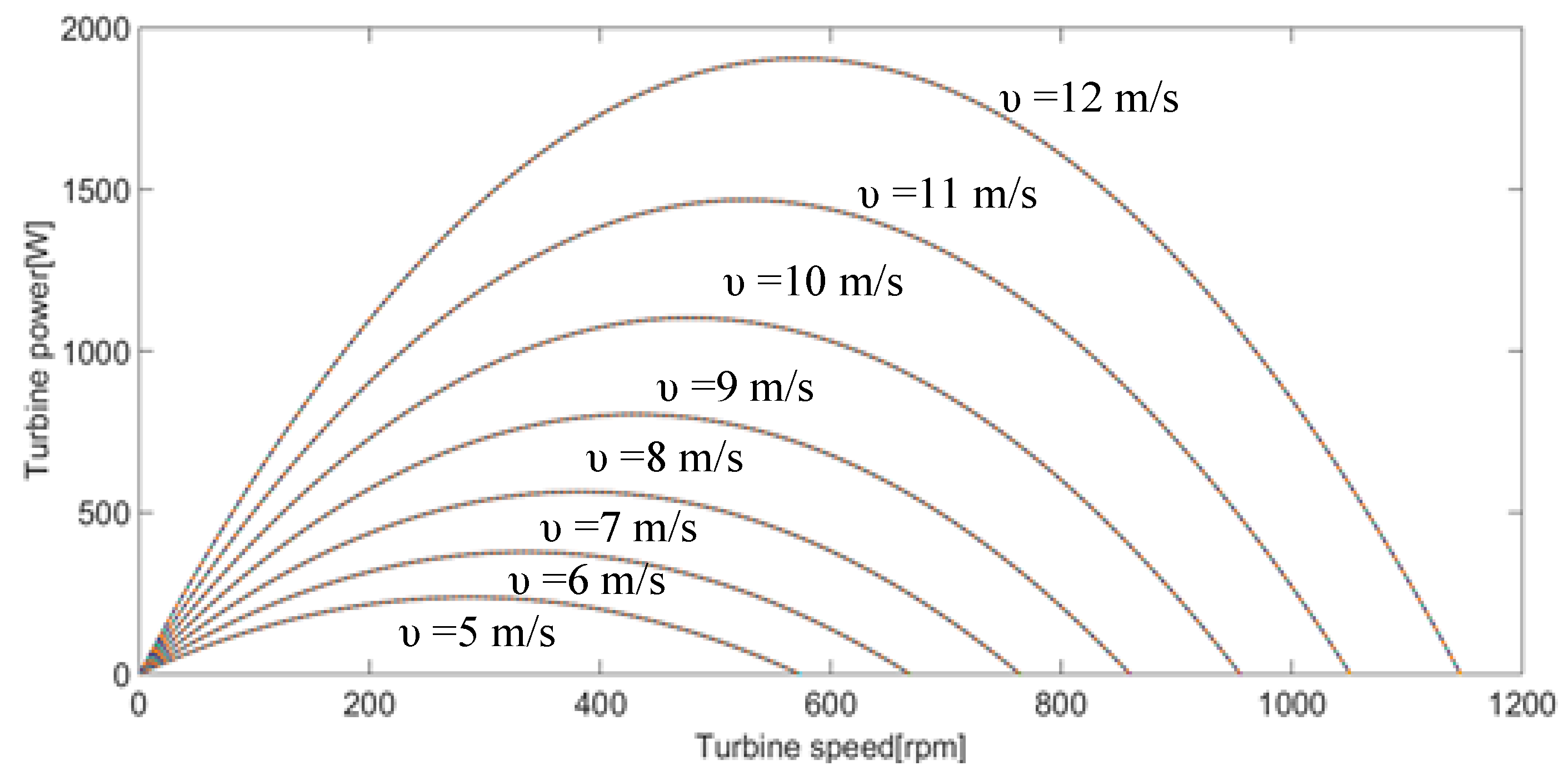
Region BC, when the wind speed is higher than the cut-in speed and less than the rated value. The output power is given by $P_{opt}=K_{opt}{\upsilon }^3$.

-

Region CD, when the rotational speed approaches to its rated value.

-

Region DE, when the wind speed is beyond the limits and the generator output power is controlled to its rated value. The blade pitch controller is activated in this region.

Figure 24a,b show the accuracy of the proposed wind estimation algorithm to estimate the wind speed. The estimation error in continuous change of wind speed is in the range of 0.2 m/s, which is considered a small value with respect to using an anemometer or measuring the average wind speed in different locations.

7. Conclusions

In this paper, a novel sensorless-based modeling for wind energy system is presented. It is developed using a torque-controlled SCIM as the wind turbine simulator. Stochastic wind speed profiles, wind shear, and torque shadow effects are simulated:

• The turbine steady-state characteristics are modeled using the turbine torque equation, which is a function of the wind speed, tip-speed ratio, and blade pitch angle.
• A derivation for the wind shear and tower shadow torque components are obtained as a function of the turbine dimensions and the estimated effective wind speed.

The main cause of system oscillations is tower shadow, wind shear shows significant oscillations on the total output torque, and the spectrum analysis shows the oscillation frequencies, which are from the third-order components. The electromagnetic transient models of DFIG and control strategies were presented and analyzed.

All the characteristics are simulated based on the estimated wind speed using the PSO-SVR method, which gives an accurate simulation of the dynamic characteristics of wind turbine.

References

1. Gan, L.K.; Shek, J.K.H.; Mueller, M.A. Modeling and characterization of downwind tower shadow effects using a wind turbine emulator. IEEE Trans. Ind. Electron. 2017, 64, 7087–7097. [Google Scholar] [CrossRef]
2. de Kooning, J.D.M.; Vandoorn, T.L.; van de Vyver, J.; Meersman, B.; Vandevelde, L. Shaft speed ripples in wind turbines caused by tower shadow and wind shear. IET Renew. Power Gener. 2014, 8, 195–202. [Google Scholar] [CrossRef]
3. Weihao, H.; Chi, S.; Zhe, C. Impact of wind shear and tower shadow effects on power system with large-scale wind power penetration. In Proceedings of the IECON 2011 37th Annual Conference of the IEEE Industrial Electronics Society, Melbourne, Australia, 7–10 November 2011; pp. 878–883. [Google Scholar]
4. Ahshan, R.; Iqbal, M.T.; Mann, G.K.I. Controller for a small induction generator-based wind turbine. Appl. Engery 2008, 85, 218–227. [Google Scholar] [CrossRef]
5. Martinez, F.; Herrero, L.C.; Pablo, S.D. Open-loop wind turbine emulator. Renew. Energy 2014, 63, 212–221. [Google Scholar] [CrossRef]
6. Kojabadi, H.M.; Chang, L.; Boutot, T. Development of a novel wind turbine simulator for wind energy conversion systems using an inverter-controlled induction motor. IEEE Trans. Energy Convers. 2004, 19, 547–552. [Google Scholar] [CrossRef]
7. Mihet-Popa, L.; Blaabjerg, F.; Boldea, I. Wind turbine generator modeling and simulation where rotational speed is the controlled variable. IEEE Trans. Ind. Appl. 2004, 40, 3–10. [Google Scholar] [CrossRef]
8. Monfared, M.; Kojabadi, H.M.; Rastegar, H. Static and dynamic wind turbine simulator using a converter controlled DC motor. Renew. Energy 2008, 33, 906–913. [Google Scholar] [CrossRef]
9. Sajadi, A.; Rosłaniec, Ł.; Kłos, M. An emulator for fixed pitch wind turbine studies. Renew. Energy 2016, 87, 391–402. [Google Scholar] [CrossRef]
10. Hughes, F.M.; Anaya-Lara, O.; Ramtharan, G. Influence of tower shadow and wind turbulence on the performance of power system stabilizers for DFIG-based wind farms. IEEE Trans. Energy Convers. 2008, 23, 519–528. [Google Scholar] [CrossRef]
11. Wan, S.; Cheng, L.; Sheng, X. Effects of yaw error on wind turbine running characteristics based on the equivalent wind speed model. Energies 2015, 8, 6286–6301. [Google Scholar] [CrossRef]
12. Tan, J.; Hu, W.; Wang, X. Effect of tower shadow and wind shear in a wind farm on AC tie-line power oscillations of interconnected power systems. Energies 2013, 6, 6352–6372. [Google Scholar] [CrossRef]
13. Shamshirband, S.; Petkovic, D.; Anuar, N.B.; Kiah, M.L.M.; Akib, S.; Gani, A.; Cojbasic, Z.; Nikolic, V. Sensorless estimation of wind speed by adaptive neuro-fuzzy methodology. Int. J. Electr. Power Energy Syst. 2014, 62, 490–495. [Google Scholar] [CrossRef]
14. Mohandes, M.; Rehman, S.; Rahman, S. Estimation of wind speed profile using adaptive neuro-fuzzy inference system (ANS). Appl. Energy 2011, 88, 4024–4032. [Google Scholar] [CrossRef]
15. Li, H.; Shi, K.; McLaren, P. Neural-network-based sensorless maximum wind energy capture with compensated power coefficient. IEEE Trans. Ind. Appl. 2015, 41, 1548–1556. [Google Scholar] [CrossRef]
16. Abo-Khalil, A.G.; Abo-Zied, H. Sensorless control for d-fig wind turbine based on support vector regression. In Proceedings of the IECON 2012 38th Annual Conference on IEEE Industrial Electronics Society, Montreal, QC, Canada, 25–28 October 2012; pp. 3475–3480. [Google Scholar]
17. Abo-Khalil, A.G.; Lee, D.C. MPPT control of wind generation systems based on estimated wind speed using SVR. IEEE Trans. Ind. Electron. 2008, 55, 1489–1490. [Google Scholar] [CrossRef]
18. Abo-Khalil, A.G. Model-based optimal efficiency control of induction generators for wind power systems. In Proceedings of the 2011 IEEE International Conference on Industrial Technology (ICIT), Auburn, AL, USA, 14–16 March 2011; pp. 191–197. [Google Scholar]
19. Abo-Khalil, A.G. Impacts of wind farms on power system stability. In Modeling and Control Aspects of Wind Power Systems; IntechOpen: London, UK, 2013; ISBN 980-953-307-562-9. [Google Scholar]
20. Abo-Khalil, A.G. Synchronization of DFIG output voltage to utility grid in wind power system. Renew. Energy 2012, 44, 193–198. [Google Scholar] [CrossRef]
21. Dolan, D.; Lehn, P. Simulation model of wind turbine 3p torque oscillations due to wind shear and tower shadow. IEEE Trans. Energy Convers. 2006, 21, 717–724. [Google Scholar] [CrossRef]
22. Manwell, J.F.; McGowan, J.G.; Rogers, A.L. Wind Energy Explained: Theory, Design and Application; Wiley: Hoboken, NJ, USA, 2010. [Google Scholar]
23. Tummala, A.; Velamati, R.K.; Sinha, D.K.; Indraja, V.; Krishna, V.H. A review on small scale wind turbines, Renew. Sustain. Energy Rev. 2016, 56, 1351–1371. [Google Scholar] [CrossRef]
24. Lei, Y.; Mullane, A.; Lightbody, G.; Yacamini, R. Modeling of the wind turbine with a doubly fed induction generator for grid integration studies. IEEE Trans. Energy Convers. 2006, 21, 257–264. [Google Scholar] [CrossRef]
25. Gregory, I.M.; Chowdhry, R.S.; McMinn, J.D.; Shaughnessy, J.D. Hypersonic Vehicle Model and Control Law Development Using H and μ Synthesis; Langley Research Center: Hampton, VA, USA, 1994.
26. Abo-Khalil, A.G.; Kim, H.G.; Lee, D.C.; Seok, J.K. Maximum output power control of wind generation system considering loss minimization of machines. In Proceedings of the 30th Annual Conference of IEEE Industrial Electronics Society, Busan, Korea, 2–6 November 2004; pp. 1676–1681. [Google Scholar]
27. Abo-Khalil, A.G.; Lee, D.C. Grid connection of doubly-fed induction generators in wind Energy conversion system. In Proceedings of the 2006 CES/IEEE 5th International Power Electronics and Motion Control Conference, Shanghai, China, 14–16 August 2006; Volume 2, pp. 1–5. [Google Scholar]
28. Park, H.G.; Abo-Khalil, A.G.; Lee, D.C.; Son, K.M. Torque ripple elimination for doubly fed induction motors under unbalanced source voltage. In Proceedings of the 2007 7th International Conference on Power Electronics and Drive Systems, Bangkok, Thailand, 27–30 November 2007; Volume 7, pp. 1301–1306. [Google Scholar]
29. Abo-Khalil, A.G.; Park, H.G.; Lee, D.C. Loss minimization control for doubly fed induction generators in variable speed wind turbines. In Proceedings of the IECON 2007 33rd Annual Conference of the IEEE Industrial Electronics Society, Taipei, Taiwan, 5–8 November 2007; pp. 1109–1114. [Google Scholar]
30. Smola, A.J.; Schölkopf, B. A tutorial on support vector regression. Stat. Comput. 2004, 14, 199–222. [Google Scholar] [CrossRef] [Green Version]
31. Nuller, K.R.; Smola, A.J.; Ratsch, G.; Scholkopf, B.; Kohlmorgen, J.; Vapnik, V. Predicting time series with support vector machine. In International Conference on Artificial Neural Networks; Springer: Berlin/Heidelberg, Germany, 1997; pp. 999–1004. [Google Scholar]
32. Senthil, M.A.; Rao, M.V.C.; Chandramohan, A. Competitive approaches to PSO algorithms via new-acceleration coefficient variant with mutation operators. In Proceedings of the Sixth International Conference on Computational Intelligence and Multimedia Applications (ICCIMA’05), Las Vegas, NV, USA, 16–18 August 2005. [Google Scholar]
33. Vukosavic, S.N.; Levi, E. Robust DSP-based efficiency optimization of a variable speed induction motor drive. IEEE Trans. Ind. Electron. 2003, 50, 560–570. [Google Scholar] [CrossRef]
34. Lin, S.W.; Ying, K.C.; Chen, S.C.; Lee, Z.J. Particle swarm optimization for parameter determination and feature selection of support vector machines. Expert Syst. Appl. 2008, 35, 1817–1824. [Google Scholar] [CrossRef]
35. Cho, K.R.; Seok, J.K.; Lee, D.C. Mechanical parameter identification of servo systems using robust support vector regression. In Proceedings of the 2004 IEEE 35th Annual Power Electronics Specialists Conference (IEEE Cat. No.04CH37551), Aachen, Germany, 20–25 June 2004; Volume 5, pp. 3425–3430. [Google Scholar]
36. Liu, H.-H.; Chang, L.-C.; Li, C.-W.; Yang, C.-H. Particle swarm optimization-based support vector regression for tourist arrivals forecasting. Comput. Intell. Neurosci. 2018, 2018, 1–13. [Google Scholar] [CrossRef]
Figure 1. Basic configuration of the proposed wind-energy conversion system (WECS).
Energies 12 01907 g001
Figure 2. Wind turbine characteristic curves: Wind turbine power (Watt) vs. rotational speed (rpm).
Energies 12 01907 g002
Figure 3. Wind shear comparison with parameter adjustment: (a) Wind shear by rotor radius; (b) wind shear by hub height; (c) wind shear with wind shear index.
Energies 12 01907 g003
Figure 4. Dimensions used in the tower shadow formula [12].
Energies 12 01907 g004
Figure 5. Wind speed pattern in front of the tower.
Energies 12 01907 g005
Figure 6. Tower shadow effect on each blade.
Energies 12 01907 g006
Figure 7. Tower shadow effect for different r.
Energies 12 01907 g007
Figure 8. Effect of distance from tower midline x on tower shadow.
Energies 12 01907 g008
Figure 9. Dynamic model of a wind turbine.
Energies 12 01907 g009
Figure 10. Block diagram for (a) induction motor control and (b) grid-side converter.
Energies 12 01907 g010aEnergies 12 01907 g010b
Figure 11. DFIG rotor-side (a) active power control, (b) reactive power control, and (c) the total control block diagram of the DFIG.
Energies 12 01907 g011
Figure 12. (a) DFIG grid-side control, (b) voltage controller block diagram.
Energies 12 01907 g012
Figure 13. Wind speed estimation process: (a) Training samples, (b) implementation process diagram.
Energies 12 01907 g013aEnergies 12 01907 g013b
Figure 14. Implementation process diagram.
Energies 12 01907 g014
Figure 15. Layout of the experimental equipment.
Energies 12 01907 g015
Figure 16. Experimental results for continuously variable wind speed: (a) Real and estimated wind speed, (b) generator speed, and (c) generator power.
Energies 12 01907 g016
Figure 17. Tower shadow and shear effects: (a) Generator torque (Nm), (b) generator power (kW).
Energies 12 01907 g017
Figure 18. Turbine torque spectrum.
Energies 12 01907 g018
Figure 19. Turbulent wind speed: (a) Wind speed, (b) generator speed, (c) generator power, (d) q-axis current, and (e) and generator torque.
Energies 12 01907 g019
Figure 20. Turbulent high wind speed and pitch angle control: (a) Wind speed, (b) generator speed, (c) generator power, (d) q-axis current, and (e) and generator torque.
Energies 12 01907 g020
Figure 21. Spectrum of the turbulent wind speed.
Energies 12 01907 g021
Figure 22. DFIG currents after synchronization: (a) Stator currents, (b) rotor currents.
Energies 12 01907 g022
Figure 23. The simulator performance in power operation modes: (a) Wind speed, (b) generator speed, (c) generator power, and (d) q-axis current.
Energies 12 01907 g023
Figure 24. Wind speed estimation accuracy: (a) Real and estimated wind speed and (b) estimation error.
Energies 12 01907 g024