The Method of Mass Estimation Considering System Error in Vehicle Longitudinal Dynamics


Abstract
:1. Introduction
2. Mass Estimation That Considers System Error in Vehicle Longitudinal Dynamics
2.1. Longitudinal Dynamics with System Error
2.2. Recursive Least Squares Model
3. Road Test
4. Mass Estimation Result
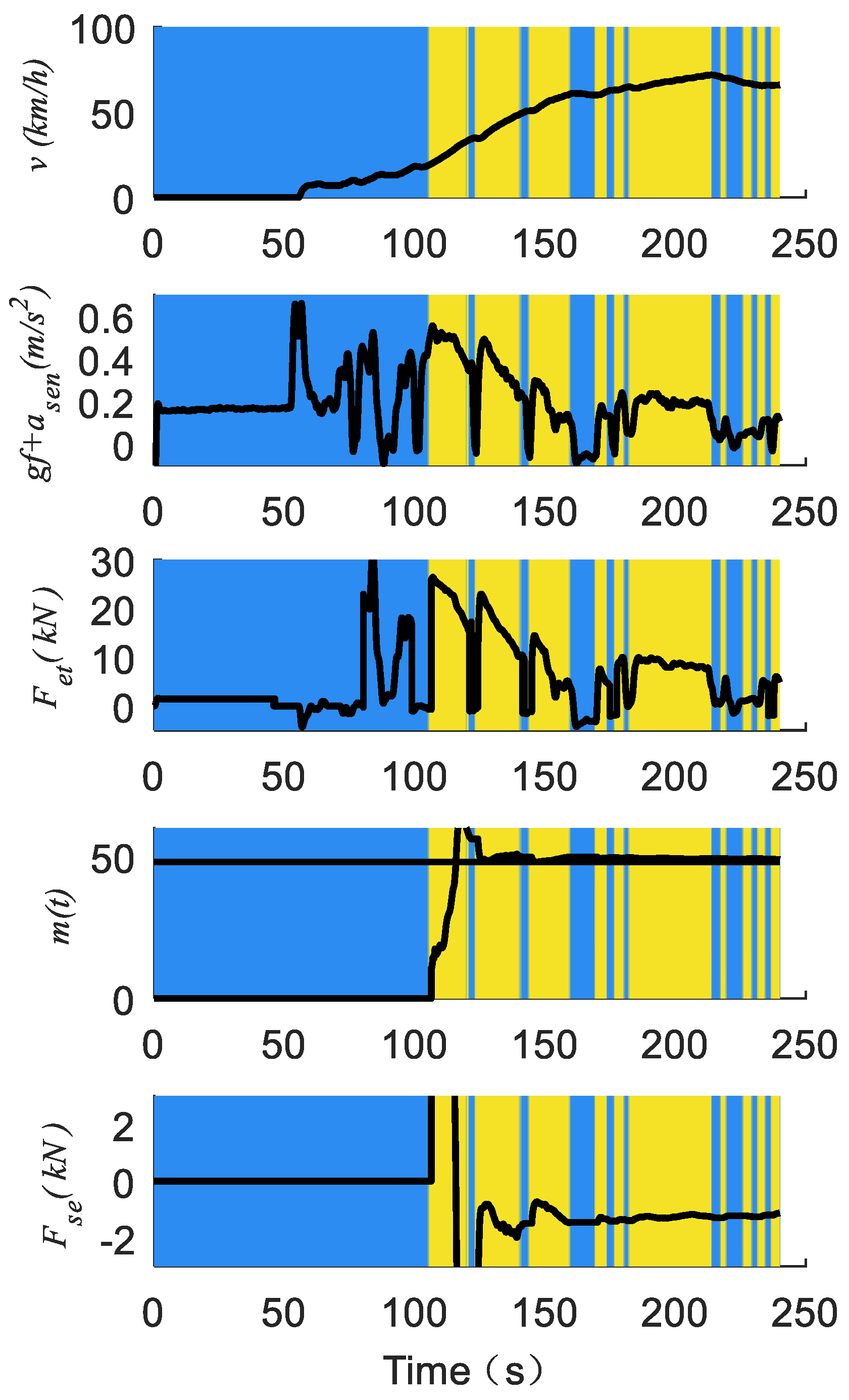
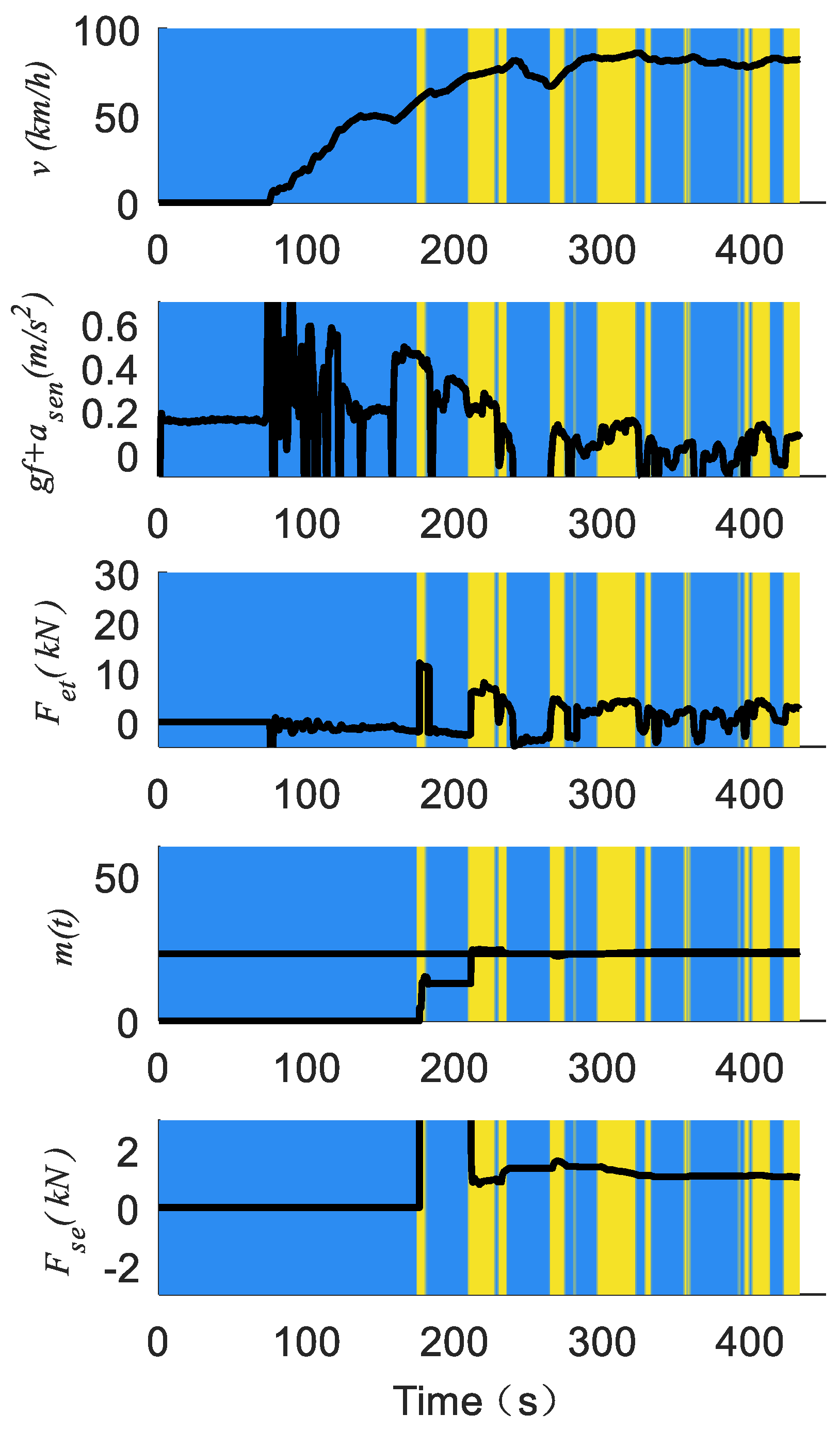
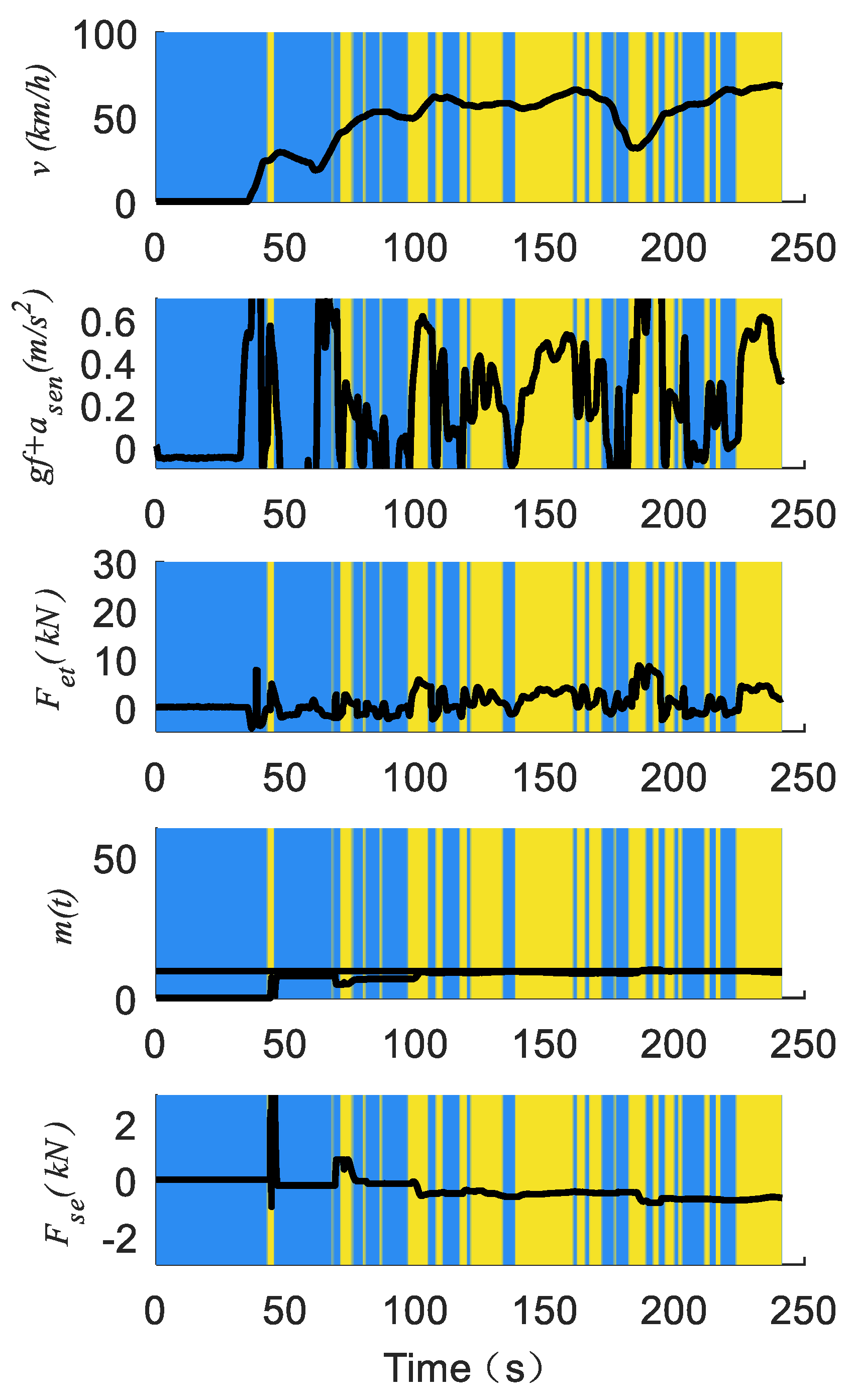
4.1. Single Test
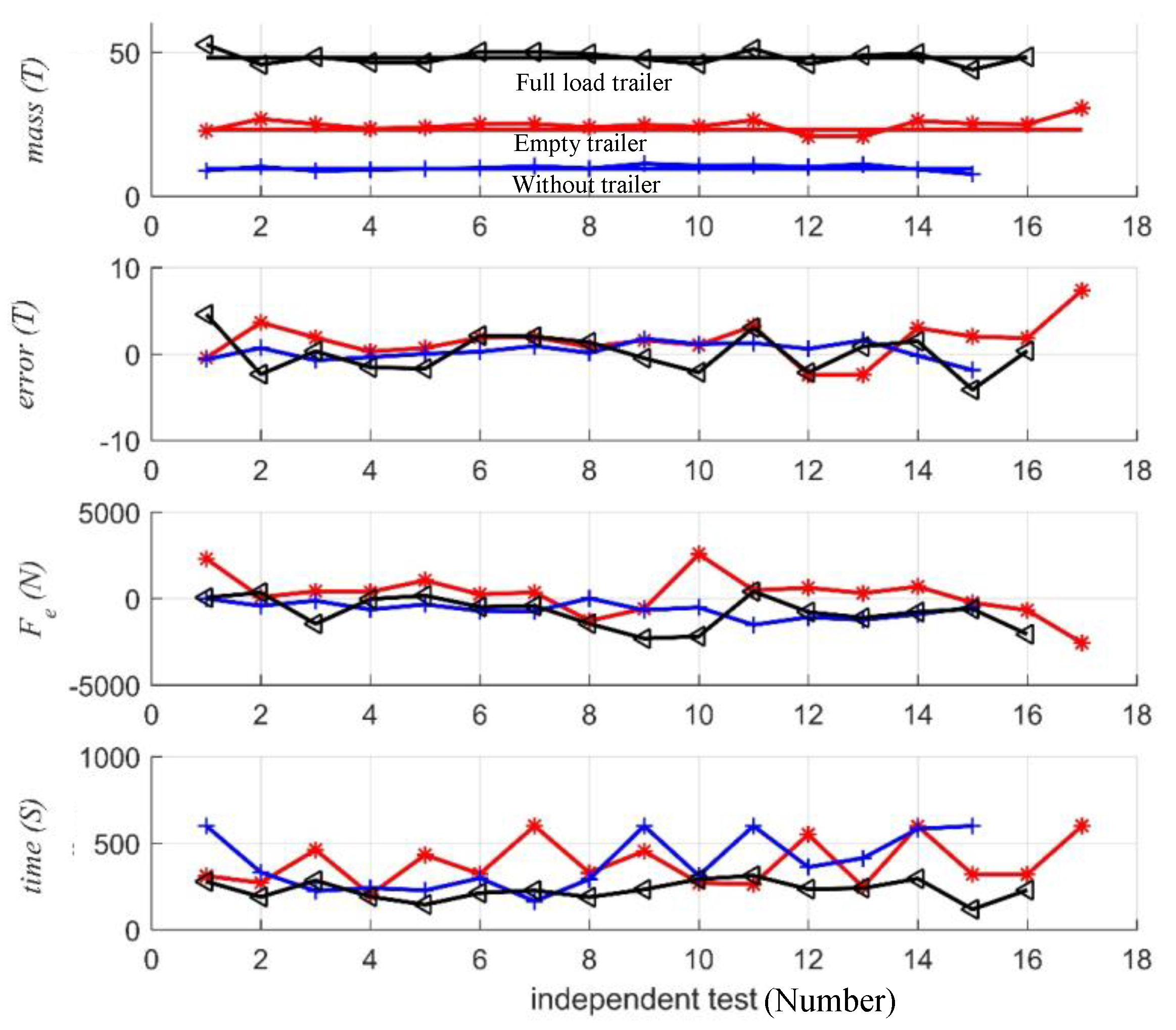
4.2. Statistical Analysis of Road Tests
5. Analysis of System Error in Vehicle Longitudinal Dynamics
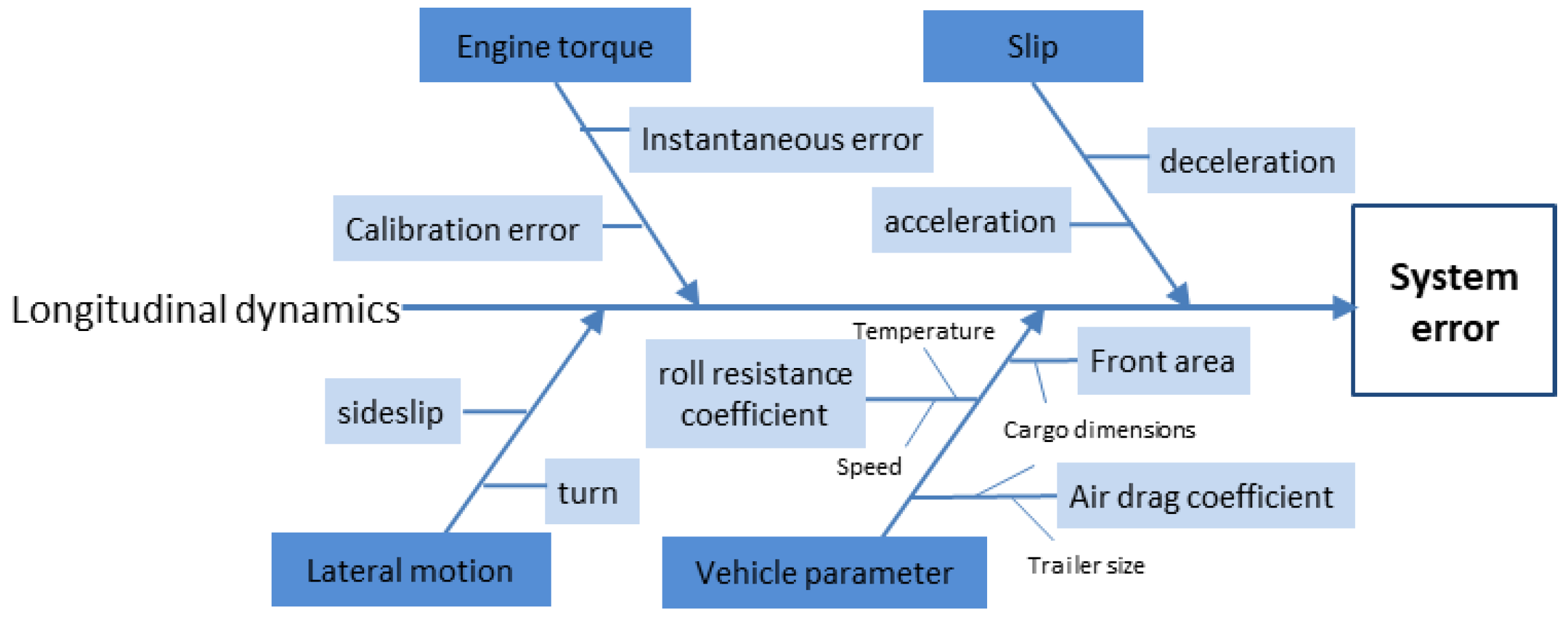
5.1. Source of System Error
5.1.1. Accuracy Limitation of Engine Torque from CAN Bus Signal
5.1.2. Constant Parameters
5.1.3. Lateral Motion and Tire Slip
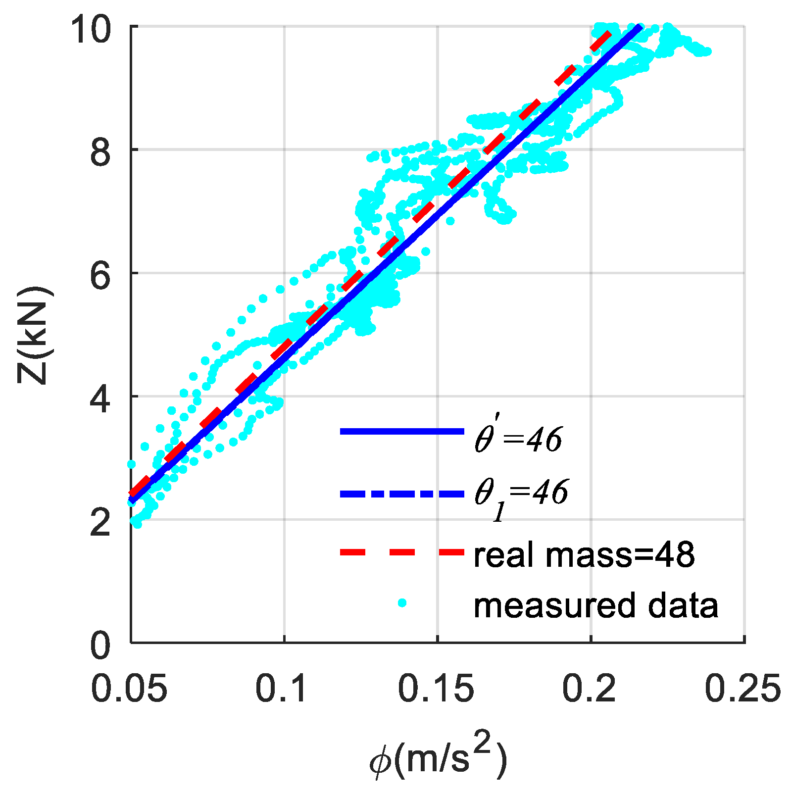
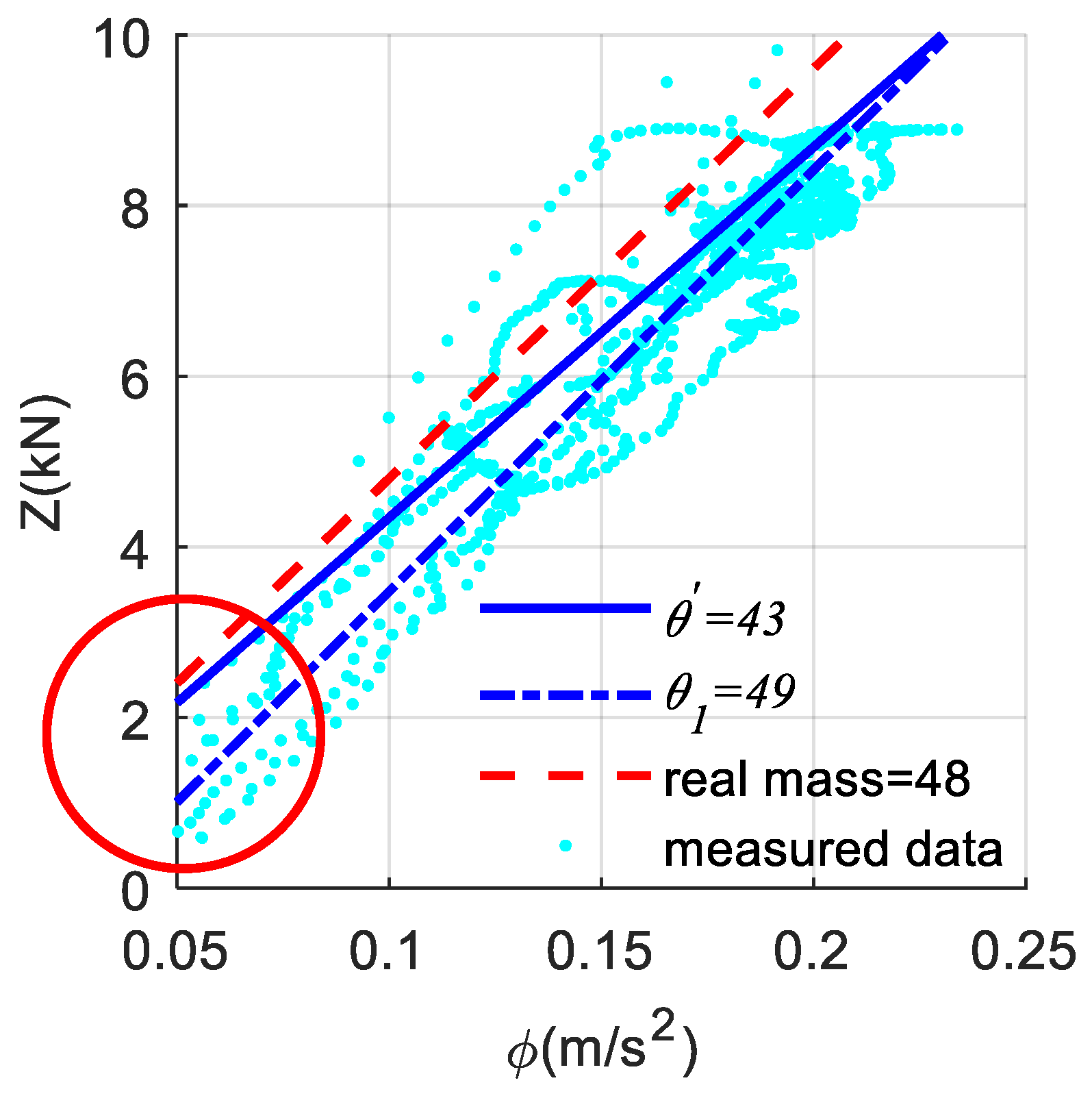
5.2. Data Fitting in Offline Situation
5.3 Comparison of the Consideration of System Error
6. Conclusions
Author Contributions
Funding
Conflicts of Interest
References
- Hayashi, K.; Shimizu, Y.; Dote, Y.; Takayama, A.; Hirako, A. Neuro fuzzy transmission control for automobile with variable loads. IEEE Trans. Control Syst. Technol. 1995, 3, 49–53. [Google Scholar] [CrossRef]
- Lin, N.; Zong, C.; Shi, S. Method for Switching between Traction and Brake Control for Speed Profile Optimization in Mountainous Situations. Energies 2018, 11, 3042. [Google Scholar] [CrossRef]
- Bae, H.S.; Gerdes, J.C. Parameter Estimation and Command Modification for Longitudinal Control of Heavy Vehicles; California Partners for Advanced Transit and Highways (PATH): San Francisco, CA, USA, 2003. [Google Scholar]
- Feng, Y.; Xiong, L.; Yu, Z.; Qu, T. Recursive least square vehicle mass estimation based on acceleration partition. Chin. J. Mech. Eng. 2014, 27, 448–459. [Google Scholar] [CrossRef]
- Eriksson, A. Implementation and Evaluation of a Mass Estimation Algorithm. Master’s Thesis, Kungliga Tekniska Högskolan, Stockholm, Sweden, 2009. [Google Scholar]
- Fathy, H.K.; Kang, D.; Stein, J.L. Online vehicle mass estimation using recursive least squares and supervisory data extraction. In Proceedings of the American Control Conference, Seattle, WA, USA, 11–13 June 2008. [Google Scholar]
- Chu, W.; Luo, Y.; Luo, J.; Li, K. Vehicle mass and road slope estimates for electric vehicles. J. Tsinghua Univ. 2014, 54, 724–728. [Google Scholar]
- Altmannshofer, S.; Endisch, C. Robust vehicle mass and driving resistance estimation. In Proceedings of the American Control Conference Boston Marriott Copley Place, Boston, MA, USA, 6–8 July 2016. [Google Scholar]
- Kidambi, N.; Pietron, G.M.; Boesch, M.; Fujii, Y. Accuracy and robustness of parallel vehicle mass and road grade estimation. SAE Int. J. Veh. Dyn. Stab. NVH 2017, 1, 317–325. [Google Scholar] [CrossRef]
- Ghosh, J.; Foulard, S.; Fietzek, R. Vehicle Mass Estimation from CAN Data and Drivetrain Torque Observer; SAE Technical Paper 2017-01-1590; SAE: Warrendale, PA, USA, 2017. [Google Scholar]
- Mahyuddin, M.N.; Na, J.; Herrmann, G.; Ren, X.; Barber, P. Adaptive observer-based parameter estimation with application to road gradient and vehicle mass estimation. IEEE Trans. Ind. Electron. 2014, 61, 2851–2863. [Google Scholar] [CrossRef]
- Mcintyre, M.L.; Ghotikar, T.J.; Vahidi, A.; Song, X.; Dawson, D.M. A two-stage lyapunov-based estimator for estimation of vehicle mass and road grade. IEEE Trans. Veh. Technol. 2009, 58, 3177–3185. [Google Scholar] [CrossRef]
- Sun, Y.; Li, L.; Yan, B.; Yang, C.; Tang, G. A hybrid algorithm combining EKF and RLS in synchronous estimation of road grade and vehicle’ mass for a hybrid electric bus. Mech. Syst. Signal Process. 2016, 68–69, 416–430. [Google Scholar] [CrossRef]
- Kidambi, N.; Harne, R.L.; Fujii, Y.; Pietron, G.M.; Wang, K.W. Methods in Vehicle Mass and Road Grade Estimation. SAE Int. J. Passeng. Cars Mech. Syst. 2014, 7, 981–991. [Google Scholar] [CrossRef]
- Wang, Z.; Qin, Y.; Gu, L.; Dong, M. Vehicle System State Estimation Based on Adaptive Unscented Kalman Filtering Combing with Road Classification. IEEE Access 2017, 5, 27786–27799. [Google Scholar] [CrossRef]
- Vahidi, A.; Stefanopoulou, A.; Peng, H. Experiments for online estimation of heavy vehicle’s mass and time-varying road grade. In Proceedings of the International Mechanical Engineering Congress and Exposition, Washington, DC, USA, 15–21 November 2003. [Google Scholar]
- Vahidi, A.; Stefanopoulou, A.; Peng, H. Recursive least squares with forgetting for online estimation of vehicle mass and road grade: Theory and experiments. Veh. Syst. Dyn. 2005, 43, 31–55. [Google Scholar] [CrossRef]
- Lei, Y.; Fu, Y.; Liu, K.; Zeng, H.; Zhang, Y. Vehicle mass and road grade estimation based on extended kalman filter. Trans. Chin. Soc. Agric. Mach. 2014, 45, 9–13. [Google Scholar]
- Yu, Y.; Kiyokawa, T.; Tsujio, S. Estimation of mass and center of mass of unknown cylinder-like object using passing-C.M. Lines. In Proceedings of the International Conference on Intelligent Robots and Systems, San Diego, CA, USA, 9 October–3 November 2001. [Google Scholar]
- Zweiri, Y.H.; Seneviratne, L.D.; Parameter, K.A. Estimation for Excavator Arm Using Generalized Newton Method. IEEE Trans. Robot. 2004, 20, 762–767. [Google Scholar] [CrossRef]
- Hong, M.; Ouyang, M. On-board torque estimation base on mean value SI engine models. J. Mech. Eng. 2009, 45, 290–294. [Google Scholar] [CrossRef]
- Yu, Z. Vehicle Theory, 4th ed.; China Machine Press: Beijing, China, 2007. [Google Scholar]
- Raffone, E. Road Slope and Vehicle Mass Estimation for Light Commercial Vehicle using linear Kalman filter and RLS with forgetting factor integrated approach. In Proceedings of the 16th International Conf. on Information Fusion Istanbul, Istanbul, Turkey, 9–12 July 2013. [Google Scholar]
- Jin, H.; Li, L.; Li, B.; Chen, H. Slope Recognition Method Based on Acceleration Interval Judgment. China J. Highw. Transp. 2010, 23, 122–126. [Google Scholar]
- Chevalier, A.; Müller, M.; Hendricks, E. On the Validity of Mean Value Engine Models during Transient Operation; SAE Technical Papers 34;2947–2951; SAE: Warrendale, PA, USA, 2000. [Google Scholar]


| Principle | Value | Reason | |
|---|---|---|---|
| 1 | Minimum speed | >5 m/s | stable running |
| 2 | Clutch engaged | <1 | tractive force output |
| 3 | Braking pedal released | <1 | no braking force |
| 4 | System input saturation (X) | 0.05 m/s2 < X < 0.8 m/s2 | eliminate abnormal data |
| 5 | System output saturation (Y) | >500 N | eliminate abnormal data |
| Constants | |||
|---|---|---|---|
| Symbol | Meaning | Unit | Value |
| η | efficiency of power train | - | 0.93 |
| r | radius of the tire | m | 0.52 |
| f | roll resistance coefficient | - | 0.0046 |
| g | acceleration of gravity | m/s2 | 9.8 |
| CDAρ | air drag coefficient (combined) | - | 10.65 |
| If | rotational inertia of the flywheel | kg·m2 | 1.7 |
| Iw | rotational inertia of all tires | kg·m2 | 398.3 |
| NO | Variables | Unit | Source |
|---|---|---|---|
| 1 | Sample time | s | CAN bus signal |
| 2 | Engine speed | rpm | |
| 3 | Engine torque | Nm | |
| 4 | Clutch signal | 0/1 | |
| 5 | Braking pedal signal | 0/1 | |
| 6 | Vehicle speed | km/h | |
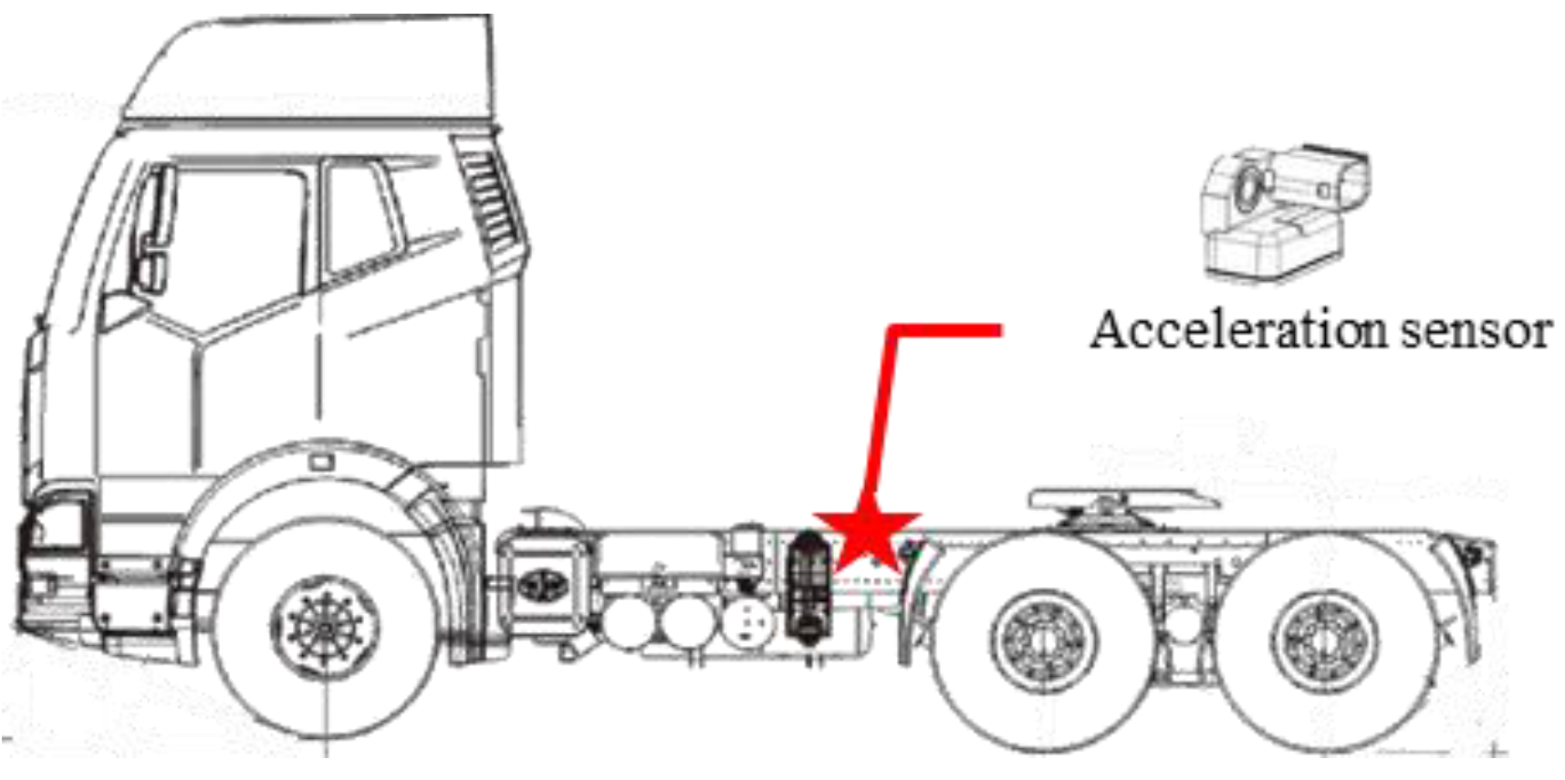
| 7 | Longitudinal acceleration | m/s2 | Acceleration sensor |
| Database | Mass (t) | Number of Tests | Notes |
|---|---|---|---|
| Tractor with full load trailer | 48.0 | 16 | - |
| Tractor with empty trailer | 23.2 | 17 | Winter test |
| Tractor without trailer | 9.5 | 15 | - |
| Tests Condition | Maximum Absolute Value (N) | Percentage within 3 t (%) | Percentage within 5 t (%) | Average | Average Absolute Value | ||
|---|---|---|---|---|---|---|---|
| Value (t) | Percentage in Real Load (%) | Value (t) | Percentage in Real Load (%) | ||||
| Full-load trailer | 4.6 | 81.3 | 100.0 | 0.1 | 0.2 | 1.9 | 4.0 |
| empty trailer | 7.3 | 82.4 | 94.1 | 1.5 | 6.5 | 2.1 | 9.1 |
| without trailer | 1.9 | 100.0 | 100.0 | 0.3 | 3.2 | 0.8 | 8.5 |
| Total | 4.6 | 87.9 | 98.0 | 0.6 | 3.3 | 1.6 | 7.2 |
| Tests Condition | Average (N) | Standard Deviation | Average of Absolute (N) | Average Percentage (%) | Average of Absolute Percentage (%) |
|---|---|---|---|---|---|
| full load trailer | −798.8 | 869.7 | 919.8 | −9.9 | 10.5 |
| empty trailer | 240.3 | 1158.5 | 872.5 | 8 | 16.8 |
| Tests Condition | Estimated Mass (t) | Error (t) | Average Absolute Error (t) | Maximum Absolute Error (t) | Average Absolute Error Percentage in Real Load (%) | |
|---|---|---|---|---|---|---|
| Full-load trailer empty trailer | θ’ = [m]T | 44.8 | −3.2 | 4.5 | 14.6 | 9.4 |
| θ = [m Fe]T | 48.1 | 0.1 | 1.9 | 4.6 | 4 | |
| without trailer full-load trailer | θ’ = [m]T | 26.9 | 3.7 | 5.3 | 19.9 | 22.8 |
| θ = [m Fe]T | 24.7 | 1.5 | 2.1 | 7.3 | 9.1 | |
| empty trailer | θ’ = [m]T | 8 | -1.5 | 1.5 | 3.5 | 15.8 |
| θ = [m Fe]T | 9.8 | 0.3 | 0.8 | 1.9 | 8.4 | |
| total | θ’ = [m]T | - | -0.3 | 3.8 | 12.7 | 16 |
| θ= [m Fe]T | - | 0.6 | 1.6 | 4.6 | 7.2 | |
© 2018 by the authors. Licensee MDPI, Basel, Switzerland. This article is an open access article distributed under the terms and conditions of the Creative Commons Attribution (CC BY) license (http://creativecommons.org/licenses/by/4.0/).
Share and Cite
Lin, N.; Zong, C.; Shi, S. The Method of Mass Estimation Considering System Error in Vehicle Longitudinal Dynamics. Energies 2019, 12, 52. https://doi.org/10.3390/en12010052
Lin N, Zong C, Shi S. The Method of Mass Estimation Considering System Error in Vehicle Longitudinal Dynamics. Energies. 2019; 12(1):52. https://doi.org/10.3390/en12010052
Chicago/Turabian StyleLin, Nan, Changfu Zong, and Shuming Shi. 2019. "The Method of Mass Estimation Considering System Error in Vehicle Longitudinal Dynamics" Energies 12, no. 1: 52. https://doi.org/10.3390/en12010052
APA StyleLin, N., Zong, C., & Shi, S. (2019). The Method of Mass Estimation Considering System Error in Vehicle Longitudinal Dynamics. Energies, 12(1), 52. https://doi.org/10.3390/en12010052