Lattice Boltzmann Simulation for the Forming Process of Artificial Frozen Soil Wall

Abstract

A lattice Boltzmann model is proposed to simulate the forming process of artificial frozen soil wall. The enthalpy method is applied to deal with the latent-heat source term, and the adjustable thermal diffusivity is utilized to handle the change of thermophysical parameters. The model is tested by the heat conduction with solid–liquid phase change in semi-infinite space, which shows a good consistence between the numerical and analytical solutions, and the mesh resolution has little effect on the numerical results. Lastly, the development of frozen soil wall is discussed when the freezing pipes are arranged in a square. The results show that the evolution of temperature field with time is closely related to the distance from the freezing pipe. For the soil near freezing pipe, the temperature gradient is larger, the soil temperature drops rapidly and freezes in a short time. The time history curve of temperature is relatively smooth. For the soil far away from freezing pipe, the temperature evolution curve has obvious multistage, which can be divided into four stages: cooling, phase change, partly frozen and completely frozen. The spacing of freezing pipes has a significant influence on the overlapping time of artificial frozen soil wall, and there is a power function relationship between them.

1. Introduction

As an effective temporary ground improvement technique, artificial ground freezing (AGF) has been widely adopted in geotechnical engineering [1,2], including departure and reception of shield tunnel, tunnels connecting passage in Metro, mine shaft sinking and municipal engineering, etc. It has advantages of strong stratum adaptability, good sealing performance, high strength and little influence on the surrounding environment. In ground improvement engineering, the development of the frozen soil wall determines its average temperature, thickness, physical and mechanical properties. These indexes reflect the strength and stability of the frozen soil wall, which is directly related to the scheduling management of projects. In the process of artificial freezing, the temperature evolution of soil is a transient heat conduction problem including ice–water phase change, latent heat release, internal heat source, moving boundary and irregular geometric boundary. The soil temperature distribution is also affected by the interaction of freezing pipes. Therefore, the forming process of frozen soil wall is very complicated, and a better understanding of heat transfer mechanisms is essentially important, which can provide necessary technical guarantees for the implementation of artificial freezing projects.

Based on the steady heat conduction theory, a large number of scholars have proposed the analytical methods of temperature evolution with a single pipe, single or double row pipes [3,4,5]. However, these methods are limited to simplified boundary conditions and idealized initial conditions. Besides, the theoretical formula is too complicated for engineering application. In recent years, numerical methods have been widely applied in heat conduction problems with phase change. Singh [6] studied the flow and heat transfer characteristics of a phase transition, melting problem. Santos [7] applied the finite element method to predict freezing times of mushrooms. Farrokhpanah [8] introduced a new smoothed particle hydrodynamics (SPH) method to model the heat transfer with phase change considering the latent heat released (absorbed) during solidification (melting). Furenes [9] used the event location algorithm in the finite difference method for phase-change problems.

When compared with the traditional numerical methods, the lattice Boltzmann method (LBM) enjoys advantages of both macroscopic and microscopic approaches [10,11]. It has clear physical conception, easy programming, high computational efficiency and is easy to apply for complex domains [12,13,14]. So, LBM has been explored to deal with heat conduction problems with phase change. Miller [15] proposed a simple model for the liquid-solid phase change based on the lattice Boltzmann method with enhanced collisions. Jiaung [16] firstly developed an enthalpy-based lattice Boltzmann model for simulating solid/liquid phase change problem governed by the heat conduction equation. Huber et al. [17,18,19] improved this model, and used it to couple thermal convection and phase change of single-component systems. Eshraghi [20] developed a new variation to solve the heat conduction with phase change by treating implicitly the latent heat source term. Huang [21] proposed a new lattice Boltzmann model to treat the latent heat source term by modifying the equilibrium distribution function. Sadeghi [22,23] proposed a three-dimensional Boltzmann model to study the film-boiling phenomenon. Chatterjee [24] extended the lattice Boltzmann formulation to simulate three-dimensional heat diffusion coupled with solid–liquid phase change. Li [25] presented a three-dimensional multiple-relaxation-time lattice Boltzmann model for the solid–liquid phase change based on the enthalpy conservation equation. The above studies mainly neglected the change of thermal diffusivity for simplifying the calculation. However, the thermal diffusivity of liquid water is only 1/9 of ice, and the water content of artificial frozen soil is generally high, so it is necessary to consider the change of thermal diffusivity during the forming process of artificial frozen soil wall.

In this paper, the enthalpy approach is applied to treat the latent heat source term in the energy equation, the adjustable thermal diffusivity is utilized to simulate the change of thermophysical parameters, and a thermal lattice Boltzmann model is proposed to simulate the forming process of artificial frozen soil wall. The model is subsequently tested with the solid–liquid phase change of pure substance in semi-infinite space. Finally, the forming process of an artificial frozen wall is simulated when the four freezing pipes are arranged in a square, the evolution of the freezing front and the temperature distribution are analyzed during the artificial freezing process, which provides the theoretical basis for the design and construction of practical engineering.

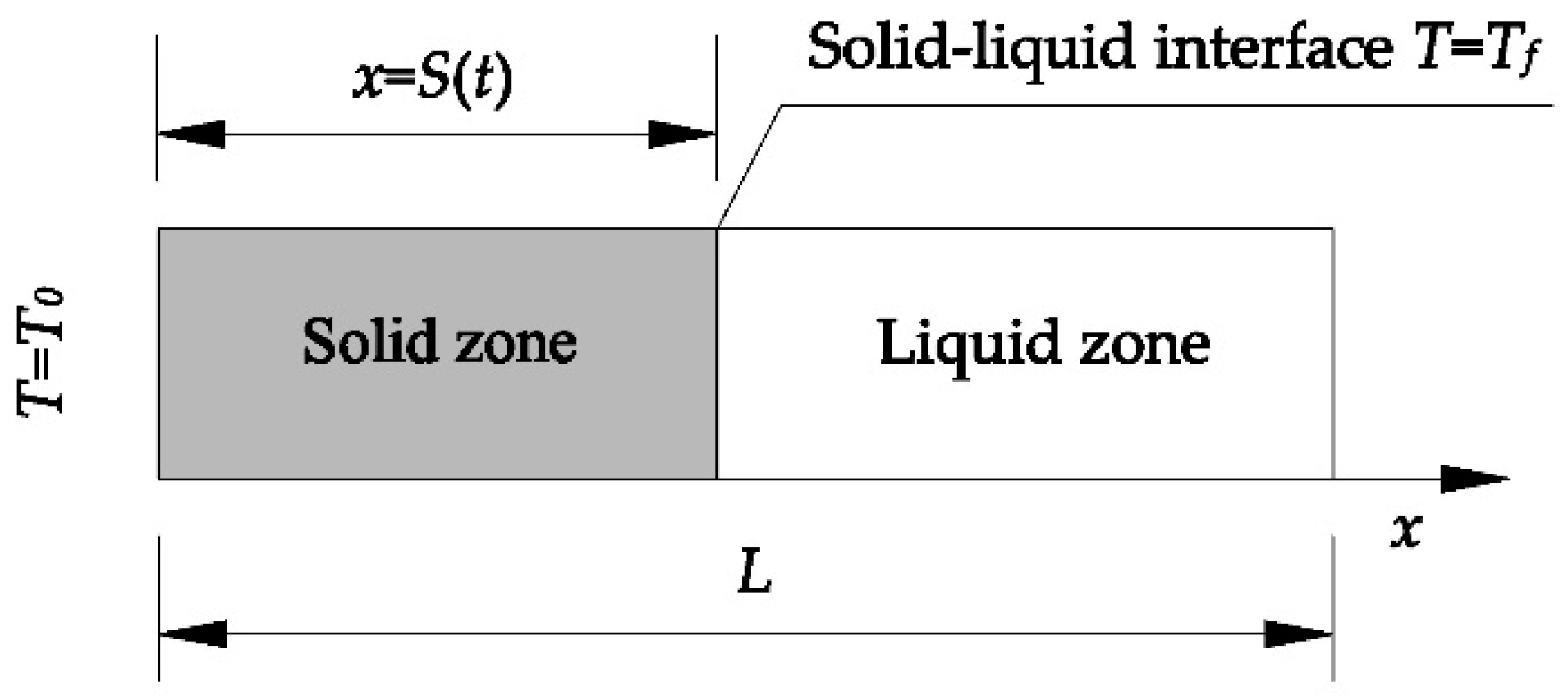
2. Heat Conduction Model of Soil Freezing

2.1. Assumptions

To develop the heat conduction model with phase change for soil, the following assumptions are made:

(1) Ignoring the influence of pore structure, soil is regard as the continuous, homogeneous and isotropic medium.

(2) According to the physical state of water, the freezing soil is divided into two parts: solid and liquid zones, and the thermophysical parameters are constant in each zone.

(3) The freezing temperature of soil is constant, and the liquid phase fraction is applied to trace the solid–liquid interface.

(4) The coupling of temperature, stress and moisture is neglected during the artificial freezing process.

2.2. Mathematical Model

Compared with the three-dimensional model, the two-dimensional one could reflect the general evolution laws and save a lot of computing resources, so it is selected in the present paper. According to energy conservation, the mathematical model of soil freezing can be expressed as [26]:

Solid phase

$$\frac{\partial T_s}{\partial t}={\alpha }_s\left[\frac{{\partial }^2{T}_s}{\partial x^2}+\frac{{\partial }^2{T}_s}{\partial y^2}\right],$$

(1)

Liquid phase

$$\frac{\partial T_l}{\partial t}={\alpha }_l\left[\frac{{\partial }^2{T}_l}{\partial x^2}+\frac{{\partial }^2{T}_l}{\partial y^2}\right],$$

(2)

The solid–liquid interface

$$\{\begin{array}{l}{T}_s=T_l\\ k_s\frac{\partial T_s}{\partial r}-k_l\frac{\partial T_l}{\partial r}={\rho }_s{L}_a\frac{\partial S}{\partial t}\end{array},$$

(3)

where $T$ is the temperature, t is the time.$\rho$, $k$ and $\alpha$ are the density, thermal conductivity and thermal diffusivity, respectively, and all these parameters can be determined by the volume fraction of each component in soil [27,28]. $L_a$ is the latent heat, $S$ is the position of solid–liquid interface. r is the normal direction of frozen front. The subscript $l$ represents that the water in the soil is the liquid phase, and $s$ the solid phase.

2.3. Phase Change Treatment

The difficulties of temperature prediction lie in the treatment of latent heat and the movement of solid–liquid interface during the soil freezing process. In this paper, the enthalpy model proposed by Shamsundar [29] is adopt to develop the unified energy equation in the whole region (including liquid zone, solid zone and solid–liquid interface), and the solid–liquid interface is determined by solving the enthalpy parameter. This model does not need to separate the solid and liquid phases, and trace the solid–liquid interface. Mathematically, it has been proved to be equivalent to the heat conduction equation with phase change [30]. So, the Equations (1)–(3) can be unified as

$$\rho \frac{\partial H}{\partial t}=k\left(\frac{{\partial }^{2}T}{\partial x^2}+\frac{{\partial }^{2}T}{\partial y^2}\right),$$

(4)

where $H$ is the total enthalpy, which can be divided into sensible and latent enthalpy components as:

$$H=C_{p}T+\varphi L_a,$$

(5)

where $C_p$ is the specific heat capacity, $\varphi$ is the liquid phase fraction, which is $0$ for solid zone, $1$ for liquid zone.

When the freezing temperature $T_f$ is constant, the relationship between the liquid phase fraction $\varphi$ and the total enthalpy $H$ can be expressed as the follows:

$$\varphi =\{\begin{array}{ll}0& H<C_p{T}_f\\ \frac{H-C_p{T}_f}{L_a}& C_p{T}_f\le H\le C_p{T}_f+L_a\\ 1& H>C_p{T}_f+L_a\end{array},$$

(6)

Substituting Equation (5) into Equation (4) yields:

$$\frac{\partial T}{\partial t}=\alpha \left(\frac{{\partial }^{2}T}{\partial x^2}+\frac{{\partial }^{2}T}{\partial y^2}\right)-\frac{L_a}{C_p}\frac{\partial \varphi }{\partial t},$$

(7)

Equation (7) is applied to describe the evolution of temperature field during the soil freezing process. In terms of the liquid phase fraction $\varphi$, the thermal diffusivity α can be expressed as:

$$\alpha =\varphi {\alpha }_l+\left(1-\varphi \right){\alpha }_s,$$

(8)

2.4. Dimensionless Treatment

To facilitate transformation between physical and lattice units, the following dimensionless parameters are introduced

$$X=\frac{x}{L},\theta =\frac{T-T_0}{T_i-T_0},F_o=\frac{{\alpha }_{s}t}{L^2},Ste=\frac{C_p\left(T_f-T_0\right)}{L_a},$$

(9)

where $X$, $\theta$ are the dimensionless coordinate and temperature. $Ste$, $F_o$ are the Stefan number and Fourier number, respectively. $L$ is the reference length, $T_0$ is the temperature of cold source, $T_i$ is the initial temperature of soil.

3. Lattice Boltzmann Model

3.1. Lattice Boltzmann Equation

The d-dimensional m-speed (DdQm) model proposed by Qian et al. [31], is the basic model of LBM. Compared with D2Q9 model, the D2Q4 model (Figure 1) has not only comparable accuracy but also better computational efficiency for temperature evolution, so it is employed to solve the heat conduction equation, which is governed by Equation (7). And the enthalpy model is adopted to treat the latent heat source term. The discrete form of the lattice Boltzmann equation can be written as:

$$g_i\left(\mathbf{r}+{\mathbf{e}}_{\mathbf{i}}{\delta }_t,t+{\delta }_t\right)-g_i\left(\mathbf{r},t\right)=-\frac{g_i\left(\mathbf{r},t\right)-g_i^{eq}\left(\mathbf{r},t\right)}{\tau }+{\omega }_{i}Sr{\delta }_t\left(i=0,1,2,3\right),$$

(10)

where $g_i\left(\mathbf{r},t\right)$ is the temperature distribution function of the ith direction at the lattice site $\mathbf{r}$ and time $t$, $g_i^{eq}\left(\mathbf{r},t\right)$ represents the equilibrium distribution function, $\tau$ is the dimensionless relaxation time, whose value should insure to be within (0.5,2) [32], ${\mathbf{e}}_{\mathbf{i}}$ is the discrete velocity in the lattice, which is composed of the velocity vectors:

$$\mathbf{e}=c\left[\begin{array}{llll}1& 0& -1& 0\\ 0& 1& 0& -1\end{array}\right],$$

(11)

where $c$ is the lattice speed, and $c={\delta }_x/{\delta }_t$, ${\delta }_x$, ${\delta }_t$ are the lattice space and time step, respectively, and they are usually taken as ${\delta }_x={\delta }_t=1$ for simplifying the calculation.

$g_i^{eq}\left(\mathbf{r},t\right)$ can be described as

$$g_i^{eq}\left(\mathbf{r},t\right)={\omega }_{i}T\left(\mathbf{r},t\right),$$

(12)

where ${\omega }_i$ is the weight factor in the $i$th direction, and ${\omega }_0={\omega }_1={\omega }_2={\omega }_3=1/4$ for D2Q4 model.

$Sr$ is the heat source term, according to Equation (7), it can be expressed as:

$$Sr=-\frac{L_a}{C_p}\frac{\partial \varphi }{\partial t},$$

(13)

Based on the first-order expansion, the heat source term $Sr$ is approximately discretized into:

$$Sr=-\frac{L_a}{C_p}\frac{\left[\varphi \left(t+{\delta }_t\right)-\varphi \left(t\right)\right]}{{\delta }_t},$$

(14)

By Chapman–Enskog expansion, Equation (10) can be recovered to the macroscopic heat conduction Equation (7), the thermal diffusivity α is given by

$$\alpha =c_s^2\left(\tau -\frac{1}{2}\right){\delta }_t,$$

(15)

where $c_s$ is lattice sound speed, for the D2Q4 model, $c_{\mathrm{s}}^2=c^2/2$.

The macroscopic temperature can be calculated as:

$$T\left(\mathbf{r},t\right)={\displaystyle \sum _{i=0}^3{g}_i\left(\mathbf{r},t\right)},$$

(16)

3.2. Boundary Conditions

The adiabatic boundary involved in the present study, is handled by the non-equilibrium extrapolation scheme, proposed by Guo et al. [33] in 2002, which has second order accuracy. The main idea of this approach is to divide the temperature distribution functions at the boundary node $N_B$ into its equilibrium and non-equilibrium parts,

$$g_i\left(N_B,t\right)=g_i^{eq}\left(N_B,t\right)+g_i^{neq}\left(N_B,t\right),$$

(17)

The equilibrium part $g_i^{eq}\left(N_B,t\right)$ can be got by Equation (12), and the non-equilibrium part $g_i^{neq}\left(N_B,t\right)$ is approximated by extrapolating from the neighboring node $N_O$,

$$g_i^{neq}\left(N_B,t\right)=g_i\left(N_O,t\right)-g_i^{eq}\left(N_O,t\right),$$

(18)

3.3. Unit Conversion

For numerical methods, it is necessary to achieve the unit conversion between physical and lattice units. In the present study, the dimensionless treatment is carried out for all the parameters, which ensures the consistency of heat transfer criterion. The non-dimensional numbers such as Stefan number and Fourier number, are used as a bridge to realize the conversion between two unit systems.

For the thermophysical parameters (latent heat $L_a$, specific heat $C_p$), the unit conversion can be achieved based on the Stefan number $Ste$.

$$Ste=\frac{C_{pp}\left(T_{fp}-T_{0p}\right)}{L_{ap}}=\frac{C_{pL}\left(T_{fL}-T_{0L}\right)}{L_{aL}},$$

(19)

where subscript $p$ represents the physical unit, and $L$ the lattice unit.

According to an artificial freezing project, the sandy silt [34] is taken as the research object. The unit conversion of thermophysical parameters is handled, and the comparison between physical and lattice units is shown in

Table 1. Comparisons of thermophysical parameters between physical and lattice units.

Unit	Latent Heat La	Thermal Diffusivity α		Heat Capacity Cp	Initial Temperature Ti	Freezing Temperature Tf	Temperature of Cold Source T0
		Solid Phase αs	Liquid Phase αl
Physical unit	121.09 kJ/kg	5.97 × 10−7 m2/s	4.86 × 10−7 m2/s	1.449 kJ/(kg·°C)	10 °C	0 °C	−30 °C
Lattice unit	1.0	0.125	0.10176	0.47865	1.0	0.75	0.0

.

For the physical time $t_p$ and lattice time steps $N$, the relationship between them can be established according to the Fourier number $F_o$.

$$F_o=\frac{{\alpha }_p{t}_p}{L_p^2}=\frac{{\alpha }_L{t}_L}{L_L^2}$$

(20)

where $t_p$ and $t_L$ are the time in physical and lattice unit, $t_L=N{\delta }_t$. $L_p$ and $L_L$ are the reference length in physical and lattice units, if $L_p$ is the length of calculation domain, then $L_L=n{\delta }_x$, $n$ is the corresponding number of lattices.

If the physical model of 4 m × 4 m is divided into a lattice of 1000 × 1000 grid cells, and the values of ${\alpha }_p$ and ${\alpha }_L$ are assigned according to Table 1. The relationship between $t_p$ and $t_L$ can be deduced as

$$t_p=\frac{{\alpha }_L{L}_p^2}{{\alpha }_p{L}_L^2}{t}_L=\frac{0.125\times 4^2}{5.97\times {10}^{-7}\times {1000}^2}{t}_L=3.35t_L,$$

(21)

It can be known that if ${\delta }_t$ is selected as 1, the physical time 1 s is corresponding to 3.35-time steps and 1 day to 25,790-time steps.

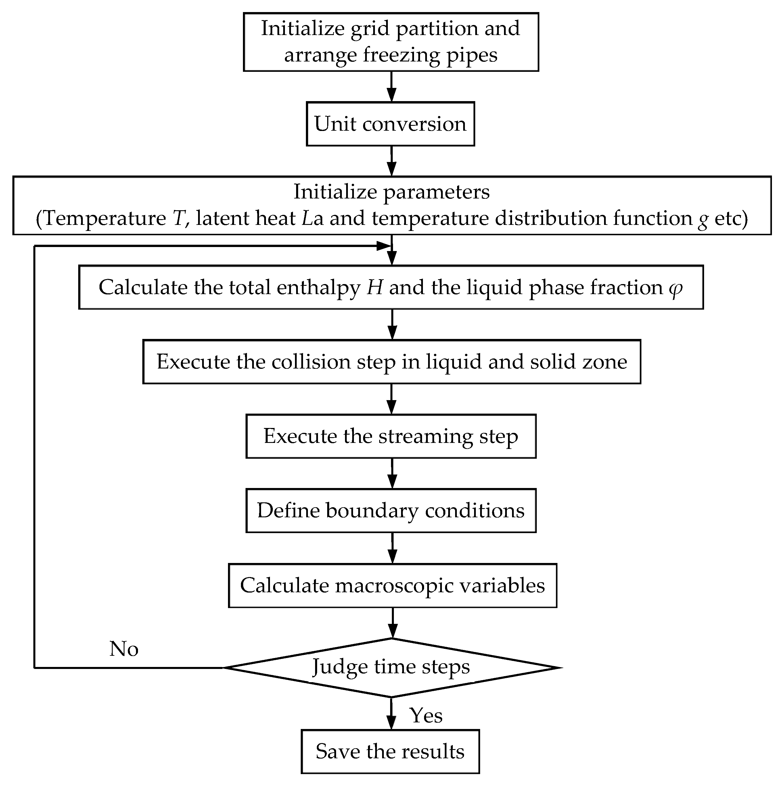
3.4. Flowchart of Program Realization

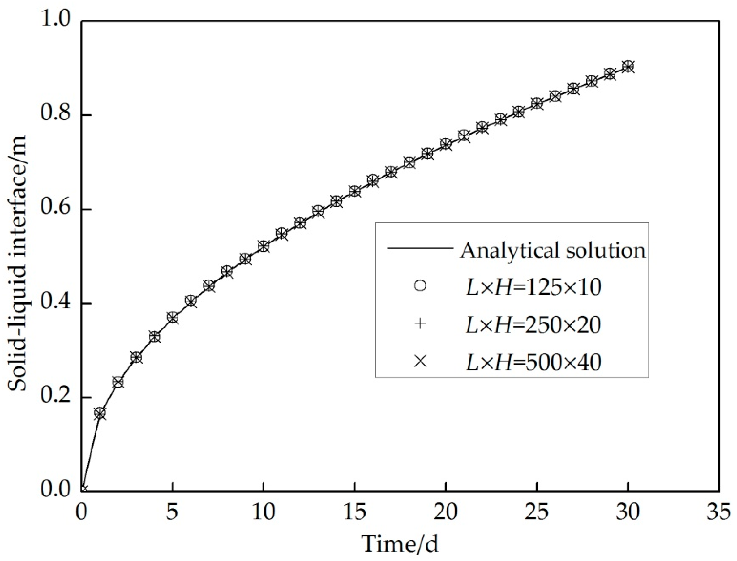
Considering the effects of heat transfer, latent heat and movement of phase-change interface during the soil freezing process, the lattice Boltzmann model is proposed based on the enthalpy method, the corresponding flowchart is shown in Figure 2.

3.5. Verification

To verify accuracy of proposed model, LBM is applied to simulate the heat conduction problem with solid–liquid phase change in semi-infinite space, as shown in Figure 3. At the time $t=0$, the uniform initial temperature is $T_i$, and the substance is in the liquid state. The cold source temperature $T_0$ is set at the position of $x=0$, and keeps constant at $t>0$. The analytical solution of the solid–liquid interface $S(t)$ and temperature $T(x,t)$ are as follows [26]

Solid–liquid interface

$$S\left(t\right)=2\lambda \sqrt{{\alpha }_{s}t},$$

(22)

Solid phase

$$T_s\left(x,t\right)=T_0+\frac{\left(T_f-T_0\right)}{erf\left(\lambda \right)}erf\left(\frac{x}{2\sqrt{{\alpha }_{s}t}}\right),$$

(23)

Liquid phase

$$T_l\left(x,t\right)=T_i+\frac{\left(T_f-T_i\right)}{erfc\left(\lambda \sqrt{\frac{{\alpha }_s}{{\alpha }_l}}\right)}erfc\left(\frac{x}{2\sqrt{{\alpha }_{l}t}}\right),$$

(24)

where $\lambda$ is the unknown parameter, which can be obtained by the following transcendental equation.

$$\frac{e^{-{\lambda }^2}}{erf\left(\lambda \right)}+\frac{k_l}{k_s}{\left(\frac{{\alpha }_s}{{\alpha }_l}\right)}^{\frac{1}{2}}\frac{\left(T_f-T_i\right)}{\left(T_f-T_0\right)}\frac{e^{-{\lambda }^2\left(\frac{{\alpha }_s}{{\alpha }_l}\right)}}{erfc\left(\lambda \sqrt{\frac{{\alpha }_s}{{\alpha }_l}}\right)}=\frac{\lambda L_a\sqrt{\pi }}{C_p\left(T_f-T_0\right)},$$

(25)

In this case, the entire domain has a size of L × H = 2 m × 0.16 m, and it is discretized using 125 × 10, 250 × 20 and 500 × 40 grid cells with lattice resolution of 16 mm, 8 mm and 4 mm, respectively. The thermophysical parameters are set according to Table 1. The temperature is fixed at T₀ on the left side, and the right boundary is adiabatic. The lattice spaces are equal in horizontal and vertical direction, ${\delta }_x={\delta }_y=1.0$ and the time step is ${\delta }_t=1.0$.

Figure 4 shows the evolution of solid–liquid interface when L × H = 125 × 10, 250 × 20 and 500 × 40, respectively. It can be seen that the results in the present study are in good agreement with the analytical ones, and the mesh resolution has little effect on the numerical results. So the proposed model can accurately simulate the movement of solid–liquid interface during the freezing process. The temperature and error distribution are shown in Figure 5 after freezing 10 days. The slope change of temperature distribution is observed at the solid–liquid interface, which is induced by the variety of thermal diffusivity. A good consistence can also be seen between the numerical results and analytical ones, which indicates the validity of the proposed model in handling the heat conduction problem with phase change. The errors are defined as the numerical solutions of temperature minus the analytical ones. As shown in Figure 5b, the errors fluctuate near the solid–liquid interface, the finer grid resolution has the smaller error, and the farther the distance from the interface, the smaller the error. The maximum errors at the interface are only −0.2 °C, 0.05 °C and 0.025 °C for L × H = 125 × 10, 250 × 20 and 500 × 40, respectively, which are acceptable for engineering application. And the lattice resolution of 4 mm is selected in the following sections.

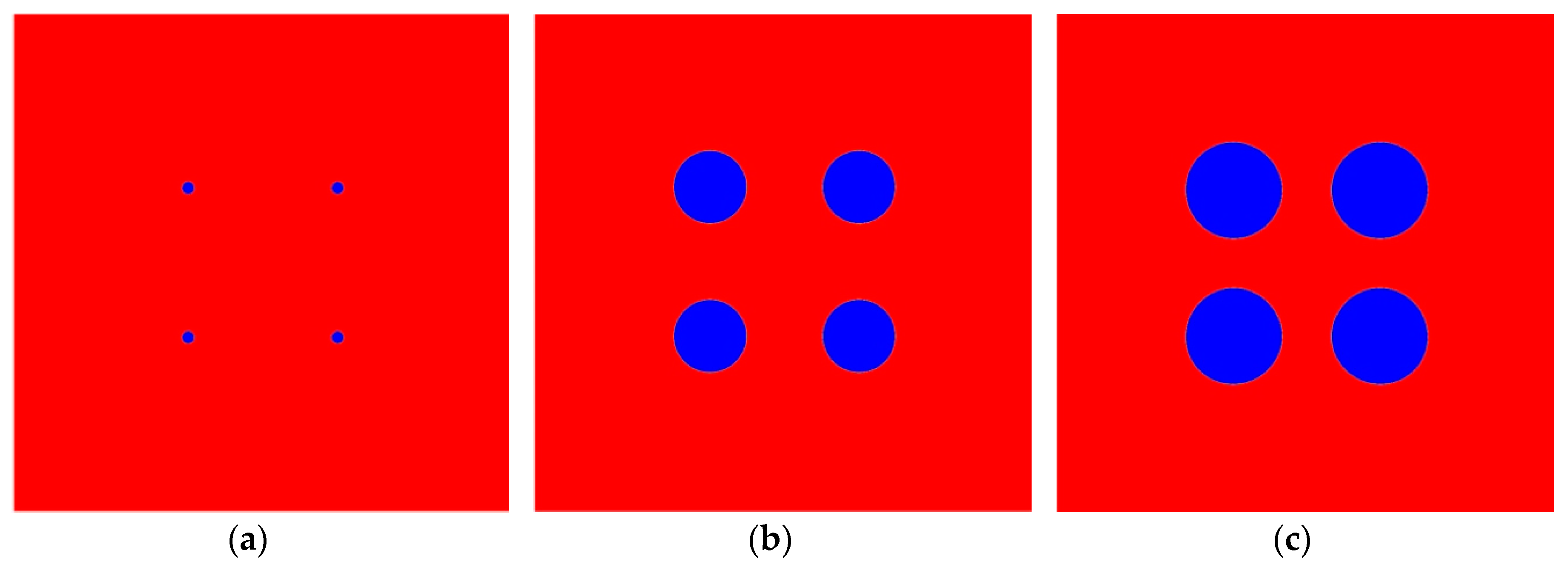
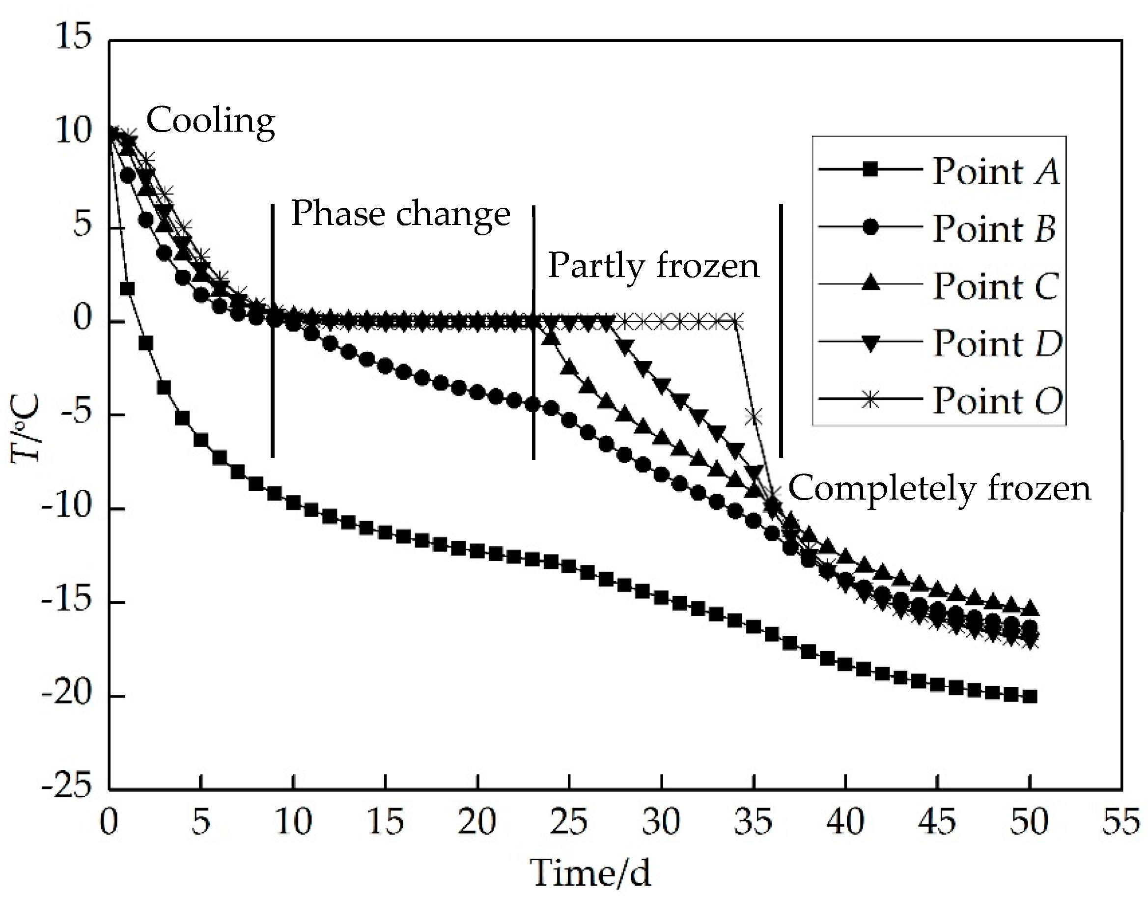
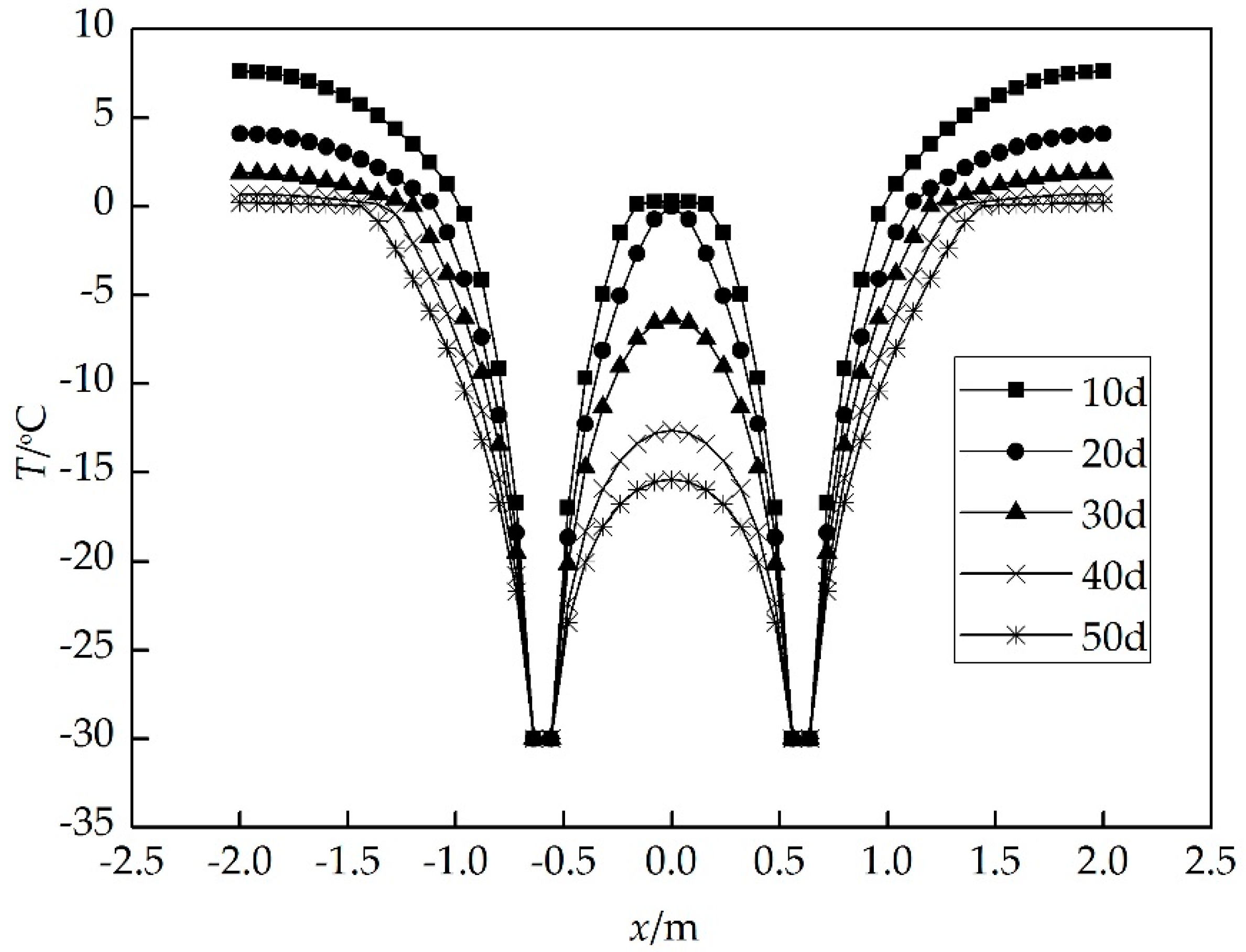
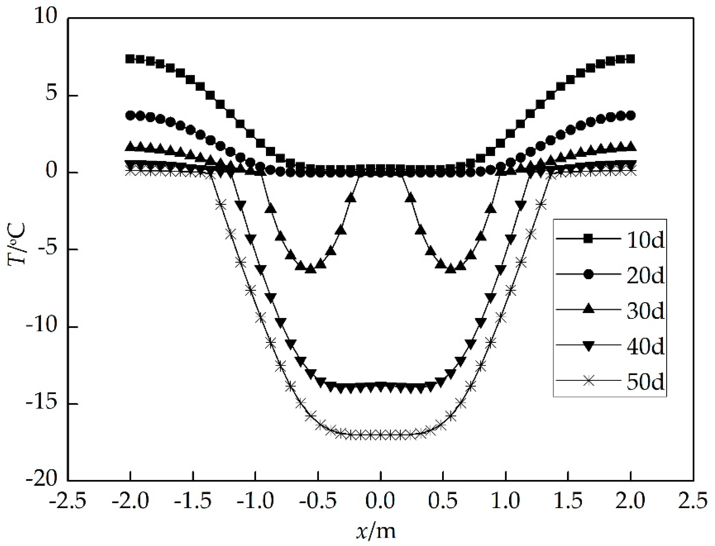
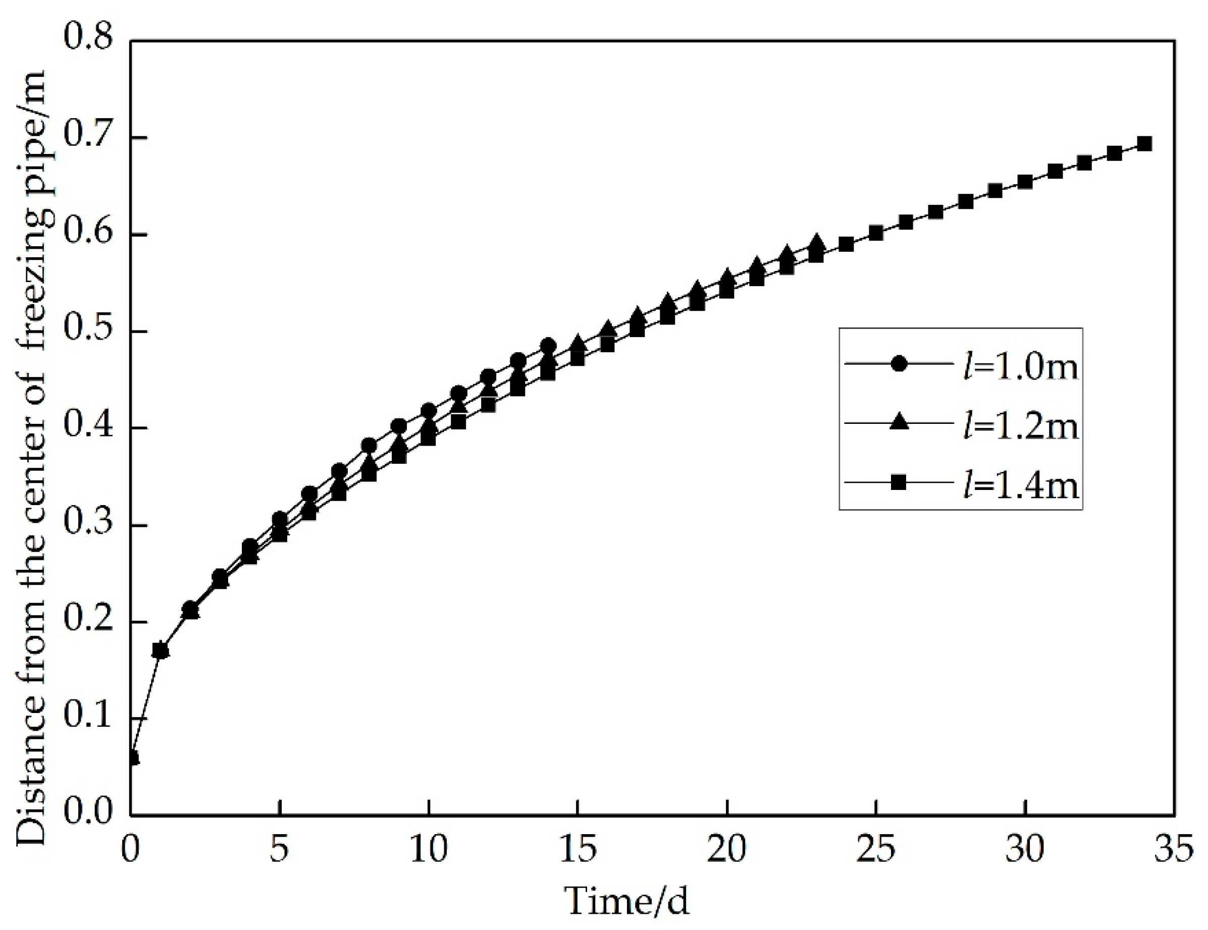
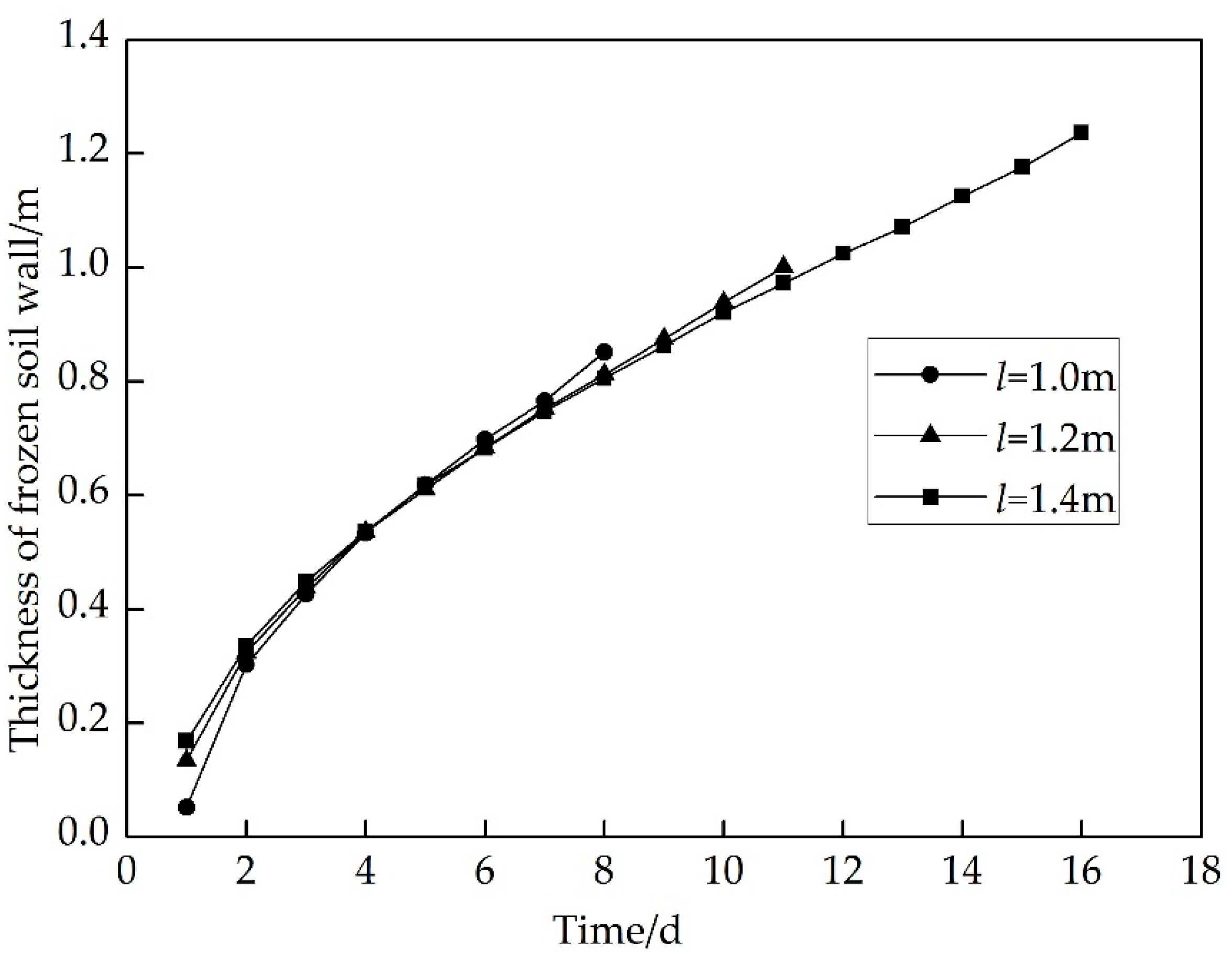
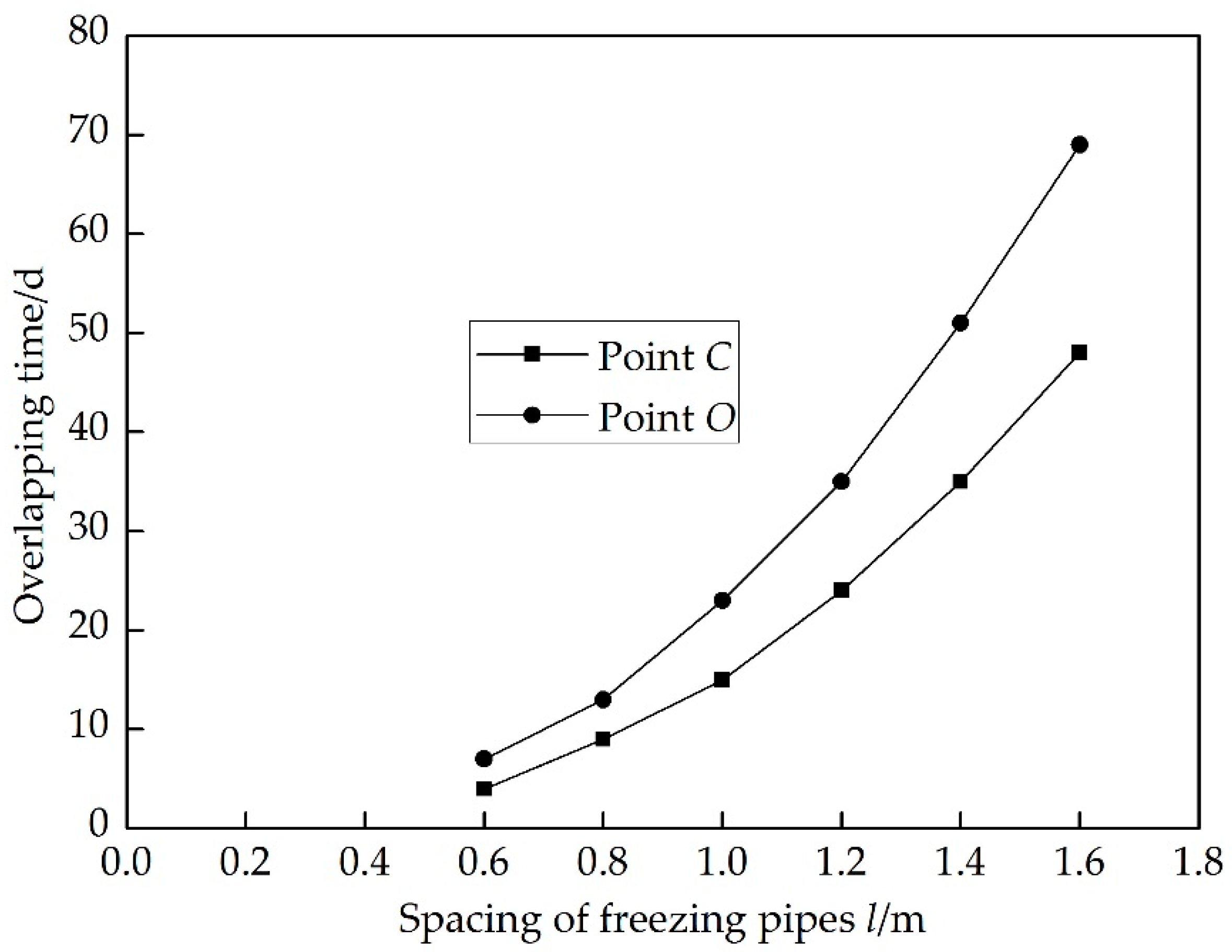
4. Results and Discussion

In practical engineering, the freezing pipes are usually arranged in a rectangular (or diamond) shape. In this paper, the four freezing pipes arranged in a square are selected as an example, which is shown in Figure 6. The development of frozen soil wall and temperature distribution are studied during the freezing process. The dimension of physical model is 4.0 m × 4.0 m. The spacing of freezing pipes is 1.2 m, and the outer diameter is 0.12 m. To ensure the mesh accuracy of the freezing pipes, the entire domain is divided into a lattice of 1000 × 1000 grid cells. The temperature of freezing pipes $T_0$ is kept at −30 °C, the freezing temperature $T_f$ is 0 °C, and the initial temperature of soil $T_i$ is 10 °C. The thermophysical parameters of soil are shown in Table 1. The freezing pipes are set as the constant temperature and the four side boundaries of the model are thermally insulated.

The temporal evolutions of frozen zone are presented in Figure 7, and the time–history curves of temperature at the points A, B, C, D and O are shown in Figure 8. It can be seen that the temperature at the point A, which is closer to the freezing pipe, has larger thermal gradient, the soil freezes quickly, the latent heat has little influence on it, and the time–history curve is smooth. The temperature at the points C, D and O, which is farther from the freezing pipe, has a similar temperature evolution trend. The time–history curves show strong multistage, and for point C it can be divided into four stages as shown in Figure 8: (1) Cooling: the temperature drops rapidly at the early stage of artificial freezing, and reaches 0 °C in about 10 days. (2) Phase change: when the temperature drops to 0 °C, soil begins to freeze and releases the latent heat. The further away from the freezing pipe, the slower the energy transfers, and the longer the persistent time of phase change stage. (3) Partly frozen: the temperature descends faster in this stage, because there is larger temperature gradient and the thermal diffusivity of frozen soil is greater than that of unfrozen soil. (4) Completely frozen: the temperature evolution is mainly affected by the thermal diffusivity of frozen soil in this stage, the overall trend is relatively stable. For the point B, the distance from freezing pipe is moderate, the temperature is somewhere in between, and shows insignificant multistage.

Figure 9 shows the temperature distribution in the main section. Under the action of freezing pipes, the soil temperature decreases rapidly in 10 days, and there is funnel-shaped distribution around the freezing pipes. In about 20 days, the frozen soil wall overlaps in the main section, after that the temperature drops rapidly until soil completely frozen between double rows of freezing pipes in about 40 days, and then the temperature decrease rate slows down gradually.

Figure 10 shows the temperature distribution in the intersection. The distance from the freezing pipes is relatively farther, so the temperature development in the intersection is obviously slower than that in the main section. In about 30 days, most of soil has been frozen in the intersection, then the temperature decreases rapidly, and the stable frozen soil wall forms in about 40 days.

The time–history curves of freezing front between two freezing pipes are present in Figure 11, which show that the closer the spacing of freezing pipe is, the faster the freezing front develops, but the whole difference is not significant. Before the frozen soil wall overlapped, the spacing of freezing pipes has little effect on the evolution of freezing front.

Figure 12 shows the thickness evolution of frozen soil wall at the point C along the x direction. The thickness develops faster at the early stage of frozen soil wall overlapped, and the developing speed gradually slows down as time goes on. In general, the thickness evolution has a similar tendency, but for the different freezing pipe spacing, there is a significant difference in overlapping time at the point O. When the spacing is 1.0 m, 1.2 m, 1.4 m, respectively, the required time for soil freezing is 8 day, 11 day and 16 day from point C to point O.

Figure 13 shows the relationship between the overlapping time and the spacing of freezing pipes. The overlapping time of frozen soil wall is greatly influenced by the spacing. The freezing times at the point C and point O increase with the increasing of the spacing, and there is a power function relationship between them. Therefore, at the design stage of artificial freezing engineering, the spacing of freezing pipes should be decided according to the overlapping time of artificial frozen soil wall.

5. Conclusion

(1) Based on the enthalpy method, a lattice Boltzmann model is proposed to simulate the heat conduction problem with phase change. The model is applied to test the solid–liquid phase change of pure substance, and the results show that the evolution of both temperature distribution and solid–liquid interface are in good agreement with the analytical solutions, and the mesh resolution has little effect on the numerical results.

(2) The temperature evolution of soil is associated with the distance from freezing pipe. When it is closer to the freezing pipe, the time–history curve of temperature is smoother, which is less affected by the latent heat. While it is farther, the time–history curve shows strong multistage, which can be divided into four stages: cooling, phase change, partly frozen, and completely frozen.

(3) Due to the effect of freezing pipes, the soil temperature in the main section decreases rapidly, there is funnel-shaped distribution around the freezing pipes, and the frozen soil wall is overlapped in about 20 days. The temperature development in the intersection is obviously slower compared with that in the main section. In about 30 days, most of soil has been frozen in the intersection, then the temperature decreases rapidly, and the stable frozen soil wall forms in about 40 days.

(4) The spacing of the freezing pipes has a significant influence on the overlapping time of artificial frozen soil wall, and there is a power function relationship between them. But it has little effect on the evolution of freezing front and the thickness of frozen soil wall.

References

1. Marwan, A.; Zhou, M.M.; Abdelrehim, M.Z.; Meschke, G. Optimization of artificial ground freezing in tunneling in the presence of seepage flow. Comput. Geotech. 2016, 75, 112–125. [Google Scholar] [CrossRef]
2. Pimentel, E.; Sres, A.; Anagnostou, G. Large-scale laboratory tests on artificial ground freezing under seepage-flow conditions. Géotechnique 2012, 62, 227–241. [Google Scholar] [CrossRef]
3. Hu, X.D.; Zhang, L.Y. Analytical solution to steady-state temperature field of two freezing pipes with different temperatures. J. Shanghai Jiaotong Univ. Sci. 2013, 18, 706–711. [Google Scholar] [CrossRef]
4. Li, F.; Xia, M. Study on analytical solution of temperature field of artificial frozen soil by exponent-integral function. J. Southeast Univ. 2004, 34, 469–473. (In Chinese) [Google Scholar]
5. Zhou, Y.; Zhou, G.Q. Analytical solution for temperature field around a single freezing pipe considering unfrozen water. J. China Coal Soc. 2012, 37, 1649–1653. (In Chinese) [Google Scholar]
6. Singh, S.; Bhargava, R. Numerical simulation of a phase transition problem with natural convection using hybrid FEM/EFGM technique. Int. J. Numer. Methods Heat Fluid Flow 2015, 25, 570–592. [Google Scholar] [CrossRef]
7. Santos, M.V.; Lespinard, A.R. Numerical simulation of mushrooms during freezing using the FEM and an enthalpy: Kirchhoff formulation. Heat Mass Transf. 2011, 47, 1671–1683. [Google Scholar] [CrossRef]
8. Farrokhpanah, A.; Bussmann, M.; Mostaghimi, J. New smoothed particle hydrodynamics (SPH) formulation for modeling heat conduction with solidification and melting. Numer. Heat Transf. Part B Fundam. 2016, 71, 299–312. [Google Scholar] [CrossRef]
9. Furenes, B.; Lie, B. Using event location in finite-difference methods for phase-change problems. Numer. Heat Transf. Part B Fundam. 2006, 50, 143–155. [Google Scholar] [CrossRef]
10. Sukop, M.C., Jr.; Thorne, D.T. Lattice Boltzmann Modeling: An Introduction for Geoscientists and Engineers; Springer: Berlin, Germany, 2010; ISBN 9783540279815. [Google Scholar]
11. Guo, Z.; Shu, C. Lattice Boltzmann method and its applications in engineering. World Sci. 2013. [Google Scholar] [CrossRef]
12. Mohamad, A.A. Lattice Boltzmann Method: Fundamentals and Engineering (Applications with Computer Codes); Springer: London, UK, 2011; ISBN 978-0-85729-454-8. [Google Scholar]
13. Chen, L. Numerical Investigation of Multiscale Multiple Physicochemical Coupled Reactive Transport Processes in Energy and Environmental Discipline. Ph.D. Thesis, Xi’an Jiaotong University, Xi’an, China, September 2013. [Google Scholar]
14. Krüger, T.; Kusumaatmaja, H.; Kuzmin, A.; Shardt, O.; Silva, G.; Viggen, E.M. The lattice Boltzmann Method: Principles and Practice; Springer: London, UK, 2017; ISBN 978-3-319-44649-3. [Google Scholar]
15. Miller, W.; Succi, S.; Mansutti, D. Lattice Boltzmann model for anisotropic liquid-solid phase transition. Phys. Rev. Lett. 2001, 86, 3578. [Google Scholar] [CrossRef] [PubMed]
16. Jiaung, W.S.; Ho, J.R.; Kuo, C.P. Lattice Boltzmann Method for the heat conduction problem with phase change. Numer. Heat Transf. Part B Fundam. 2001, 39, 167–187. [Google Scholar] [CrossRef]
17. Huber, C.; Parmigiani, A.; Chopard, B.; Manga, M.; Bachmann, O. Lattice Boltzmann model for melting with natural convection. Int. J. Heat Fluid Flow 2008, 29, 1469–1480. [Google Scholar] [CrossRef]
18. Chatterjee, D.; Chakraborty, S. An enthalpy-source based lattice Boltzmann model for conduction dominated phase change of pure substances. Int. J. Therm. Sci. 2008, 47, 552–559. [Google Scholar] [CrossRef]
19. Huo, Y.; Rao, Z. Lattice Boltzmann simulation for solid-liquid phase change phenomenon of phase change material under constant heat flux. Int. J. Heat Mass Transf. 2015, 86, 197–206. [Google Scholar] [CrossRef]
20. Eshraghi, M.; Felicelli, S.D. An implicit lattice Boltzmann model for heat conduction with phase change. Int. J. Heat Mass Transf. 2012, 55, 2420–2428. [Google Scholar] [CrossRef]
21. Huang, R.; Wu, H.; Cheng, P. A new lattice Boltzmann model for solid-liquid phase change. Int. J. Heat Mass Transf. 2013, 59, 295–301. [Google Scholar] [CrossRef]
22. Sadeghi, R.; Shadloo, M.S. Three-dimensional numerical investigation of file boiling by the lattice Boltzmann method. Numer. Heat Transf. Part A Appl. 2017, 71, 560–574. [Google Scholar] [CrossRef]
23. Sadeghi, R.; Shadloo, M.S.; Jamalabadi, M.Y.A.; Karimipour, A. A three-dimensional lattice Boltzmann model for numerical investigation of bubble growth in pool boiling. Int. J. Heat Mass Transf. 2016, 79, 58–66. [Google Scholar] [CrossRef]
24. Chatterjee, D.; Chakraborty, S. An enthalpy-based lattice Boltzmann model for diffusion dominated solid–liquid phase transformation. Phys. Lett. A 2005, 341, 320–330. [Google Scholar] [CrossRef]
25. Li, D.; Tong, Z.X.; Ren, Q.; He, Y.L.; Tao, W.Q. Three–dimensional lattice Boltzmann models for solid–liquid phase change. Int. J. Heat Mass Transf. 2017, 115, 1334–1347. [Google Scholar] [CrossRef] [Green Version]
26. Latif, M.J. Heat Conduction, 2nd ed.; Springer: Berlin, Germany, 2009; ISBN 9783642012662. [Google Scholar]
27. Côté, J.; Konrad, J.M. A generalized thermal conductivity model for soils and construction materials. Can. Geotech. J. 2005, 42, 443–458. [Google Scholar] [CrossRef]
28. Chen, P.P.; Bai, B. SPH numerical simulation of moisture migration caused by temperature in unsaturated soils. Eng. Mech. 2016. [Google Scholar] [CrossRef]
29. Shamsundar, N.; Sparrow, E.M. Analysis of multidimensional conduction phase change via the enthalpy Model. ASME Trans. J. Heat Transf. 1975, 97, 333–340. [Google Scholar] [CrossRef]
30. Guo, K. Numerical Heat Transfer; Anhui Science and Technology Publishing House: Hefei, China, 1987. (In Chinese) [Google Scholar]
31. Qian, Y.H.; D’Humières, D.; Lallemand, P. Lattice BGK model for Navier-Stokes equation. Eur. Lett. 2007, 17, 479. [Google Scholar] [CrossRef]
32. Wang, M.; Pan, N.; Wang, J.; Chen, S. Mesoscopic simulations of phase distribution effects on the effective thermal conductivity of microgranular porous media. J. Colloid Interface Sci. 2007, 311, 562–570. [Google Scholar] [CrossRef] [PubMed] [Green Version]
33. Zhaoli, G.; Chuguang, Z.; Baochang, S. Non-equilibrium extrapolation method for velocity and pressure boundary conditions in the lattice Boltzmann method. Chin. Phys. 2002, 11, 366–374. [Google Scholar] [CrossRef]
34. Qiu, F. Studies on Basic Theories and Technologies for Artificial Thawing of Artificial Frozen Soil. Master’s Thesis, Tongji University, Shanghai, China, March 2011. [Google Scholar]
Figure 1. D2Q4 model.
Energies 12 00046 g001
Figure 2. Flowchart of program realization for soil freezing.
Energies 12 00046 g002
Figure 3. Diagram of heat conduction problem with phase change in semi-infinite space.
Energies 12 00046 g003
Figure 4. Comparisons between lattice Boltzmann method (LBM) and analytical solutions for the solid–liquid interface.
Energies 12 00046 g004
Figure 5. Comparisons between LBM and analytical solutions. (a) Temperature distribution; (b) Error distribution.
Energies 12 00046 g005
Figure 6. Schematic diagram of the calculation model.
Energies 12 00046 g006
Figure 7. The temporal evolutions of frozen soil wall. (a) 0 day; (b) 5 day; (c) 10 day; (d) 20 day; (e) 30 day; (f) 40 day.
Energies 12 00046 g007aEnergies 12 00046 g007b
Figure 8. The time–history curves of temperature at the points A, B, C, D and O.
Energies 12 00046 g008
Figure 9. Temperature distribution in the main section.
Energies 12 00046 g009
Figure 10. Temperature distribution in the intersection.
Energies 12 00046 g010
Figure 11. The time–history curve of freezing front.
Energies 12 00046 g011
Figure 12. The thickness evolution of frozen soil wall.
Energies 12 00046 g012
Figure 13. Relationship between the overlapping time and the spacing of freezing pipes.
Energies 12 00046 g013