Abstract
China’s energy consumption issues are closely associated with global climate issues, and the scale of energy consumption, peak energy consumption, and consumption investment are all the focus of national attention. In order to forecast the amount of energy consumption of China accurately, this article selected GDP, population, industrial structure and energy consumption structure, energy intensity, total imports and exports, fixed asset investment, energy efficiency, urbanization, the level of consumption, and fixed investment in the energy industry as a preliminary set of factors; Secondly, we corrected the traditional principal component analysis (PCA) algorithm from the perspective of eliminating “bad points” and then judged a “bad spot” sample based on signal reconstruction ideas. Based on the above content, we put forward a robust principal component analysis (RPCA) algorithm and chose the first five principal components as main factors affecting energy consumption, including: GDP, population, industrial structure and energy consumption structure, urbanization; Then, we applied the Tabu search (TS) algorithm to the least square to support vector machine (LSSVM) optimized by the particle swarm optimization (PSO) algorithm to forecast China’s energy consumption. We collected data from 1996 to 2010 as a training set and from 2010 to 2016 as the test set. For easy comparison, the sample data was input into the LSSVM algorithm and the PSO-LSSVM algorithm at the same time. We used statistical indicators including goodness of fit determination coefficient (R2), the root means square error (RMSE), and the mean radial error (MRE) to compare the training results of the three forecasting models, which demonstrated that the proposed TS-PSO-LSSVM forecasting model had higher prediction accuracy, generalization ability, and higher training speed. Finally, the TS-PSO-LSSVM forecasting model was applied to forecast the energy consumption of China from 2017 to 2030. According to predictions, we found that China shows a gradual increase in energy consumption trends from 2017 to 2030 and will breakthrough 6000 million tons in 2030. However, the growth rate is gradually tightening and China’s energy consumption economy will transfer to a state of diminishing returns around 2026, which guides China to put more emphasis on the field of energy investment.
1. Introduction
China is a major energy consumer. Since the first half of 2018, coal, natural gas, petrol, and electricity consumption has been on the rise, among which the highest increase was coal consumption with an increase of 3.1%, and we found thermal power was a major factor of the continued growth of coal consumption. According to “BP Statistical Review of World Energy” [1], China’s renewable energy consumption accounts for 36% of global volume in 2017, among which natural gas consumption accounted for 32.6% of global natural gas consumption. This showed that China’s energy consumption has an important role in world energy consumption. At present, China’s energy consumption structure upgraded gained initial success, however there is still a distance from the long-term goal to build a low-carbon clean energy consumption structure. Therefore, based on a multitude of influencing factors of energy consumption, it is imperative to apply highly accurate predictive model to forecast energy consumption, and then study more economic information about China’s energy consumption. A high-precision energy consumption forecasting model can provide a quantitative basis for decision-making by relevant Chinese institutions, enabling China to better understand energy consumption trends and solve energy-related problems such as pollutant emissions and carbon emissions. In this article, a breakthrough is made in the machine intelligence algorithm. The PSO-LSSVM forecasting model optimized by the Tabu search algorithm is put forward, which avoids PSO-LSSVM falling into local optimum and speeds up the global search at the same time. Finally, the comparison of various forecasting models proves the fact that the accuracy and generalization ability of the TS-PSO-LSSVM forecasting model proposed in this article is higher than the others.
Energy consumption can be influenced by many factors directly or indirectly. Up to now, there are many factors affecting energy consumption have been studied [2,3,4,5,6]. Energy consumption problem is a complex nonlinear problem. So far, scholars have proposed various forecasting models, including grey prediction theory [7,8,9], multiple regression [10,11,12], input-output method [13,14], and time-series forecasting models [15,16].
Hsu et al. [7] applied artificial neural network and an improved gray model to predict electricity consumption of Taiwan, and the examples showed that the improved grey prediction model has higher prediction accuracy. Sehgal, V et al. [10] proposed the wavelet-bootstrap-multiple linear regression (WBMLR) predictive model to forecast India Mahathir Power Load Nadi River Basin, and the examples showed that the model owns higher accuracy than the artificial neural networks (ANN), wide area network (WAN), machine learning in R (MLR) model. Erdogdu E [16] applied co-integration analysis and auto-regressive integrated moving average (ARIMA) model to predict power load of the Republic of Turkey, and proved the high power load forecasting officially.
Up to now, a multitude of scholars have proposed robustness problem of the principal component analysis (PCA) based on various ways and put forward their own optimized algorithm. Luong et al. [17] considered a new method named online robust principal component analysis (RPCA) for time-varying decomposition problems and proposed a compressive online RPCA algorithm that can combine various information about decomposed vectors via an n − l1 minimization method. Chretien et al. [18] proposed a robust principal component analysis (RPCA) method to build the Low Rank + Sparse models when the used data is corrupted by outliers and applied it to estimate the topology in power grid networks. Sadeghian et al. [19] thought that traditional robust principal component analysis (RPCA) algorithms only focused on output outliers, however, both input and output data can make mistakes in developing soft sensors. They built a robust probabilistic predictive model to overcome this problem by appropriate formulation of noise distributions. Wu et al. [20] proposed a multi-component groups sparse RPCA model to solve the problems under the condition of complex dynamic background and applied alternating direction method of multipliers algorithm to the proposed model. Experiments demonstrated that the proposed method has better performance than others.
Along with the wide application of intelligent algorithms, more and more scholars have proposed various intelligent algorithms in all areas. Least squares support vector machine (LSSVM) prediction algorithm is one of the most widely used and has high accuracy and applicability. Roushangar et al. [21] built three types of models about flow characteristics, flow and bedform characteristics, and sediment characteristics based on the Least Squares Support Vector Machine optimized by Particle Swarm Optimization (PSO-LSSVM) and proved the forecasting model can predict the roughness coefficient precisely. Huan et al. [22] proposed a forecasting model based on integrated empirical mode decomposition (EEMD) and Least Squares Support Vector Machine (LSSVM) and showed that EEMD-LSSVM model is a better predictor algorithm than wavelet denoising least squares support machine (WD-LSSVM) and traditional LSSVM. Xue [23] optimized the LSSVM by improved particle swarm optimization algorithm (IMPSO-LSSVM) and proposed the combined concrete compressive strength prediction model. Then, he compared IMPSO-LSSVM, PSO-LSSVM, GA-LSSVM (the Least Squares Support Vector Machine optimized by genetic algorithm) and back-propagation neural network to prove the proposed model is an effective tool to forecast concrete compressive strength. Lu et al. [24] presented a new forecasting model based on empirical mode decomposition integrated permutation entropy (EEMD-PE), LSSVM, and gravitational search algorithm (GSA) to overcome the nonlinear prediction of wind power and volatility difficulties and predicted ultra-short-term forecasting of wind power accurately. Zhao et al. [25] used the salp swarm algorithm (SSA) on LSSVM to optimize two machine parameters in LSSVM algorithm, and showed that the forecasting model have higher accuracy than traditional LSSVM, PSO-LSSVM and BP neural network through integrated statistical indicators. Wen et al. [26] proposed the GA-LSSVM prediction model to predict landslide displacement and showed that the model can predict high-precisive consistency between measured displacement and predicted displacement. Liu et al. [27] proposed an improved gravitational search algorithm (AC-GSA) to improve the performance of GSA and optimize LSSVM parameters. They used a novel model to forecast heat rate of a 600 MW supercritical steam turbine unit. Results indicate that the AC-GSA–LSSVM model is a powerful technique to forecast load. Gorjaei et al. [28] applied the LSSVM model to predict liquid flow rate for two-phase flow through wellhead chokes and used particle swarm optimization (PSO) to optimize two parameters of the LSSVM algorithm. The PSO-LSSVM model is excellently consistent with actual measured rates. Results indicated that the PSO-LSSVM model demonstrated better regression precision and generalization capability. Zhang [29] proposed a hybrid model that combines fuzzy clustering (FC), LSSVM, and the wolf pack algorithm (WPA), and used two cases to train and test data. The results proved that the proposed model obtains higher prediction accuracy and stability.
In recent years, the Tabu search algorithm is widely used to shorten the computing time of the algorithm [30,31,32,33]
Peng et al. [30] added a Tabu search procedure into the framework of path relinking to generate solutions to the job shop scheduling problem (JSP). The results showed that Tabu search/Path relinking (TS/PR) obtained better performance than the traditional state-of-the-art algorithms for JSP. Escobar et al. [31] proposed a hybrid Granular Tabu Search algorithm to solve the Multi-Depot Vehicle Routing Problem (MDVRP). The results of cases showed that the proposed algorithm solved problems with short computing time and got best solutions. Li et al. [32] applied a hybrid algorithm (HA) to the genetic algorithm (GA) and used Tabu search (TS) at the same time to solve the flexible job shop scheduling problem with the aim to minimize the make span and proved that the proposed method can provide the best solutions. Sicilia et al. [33] presented a novel algorithm to solve the problem of the capillary distribution of goods in major urban areas. The proposed Tabu search algorithm can minimize the wide variety of constraints and complexities and reduced costs, which made problems quickly solved in time.
In order to accurately predict China’s energy consumption, this article proposes a native PSO-LSSVM model optimized by the Tabu search algorithm based on robust principal component analysis. The innovations of this article are as follows:
(1) Energy consumption is a macroeconomic issue and is affected by many influencing factors. In order to achieve accurate prediction of China’s energy consumption, based on a large amount of literature research, combined with China’s energy consumption characteristics, we selected GDP, population, industrial structure, energy consumption structure, energy intensity, total import and export, social fixed Asset investment, energy utilization rate, urbanization rate, household consumption level, and fixed investment in energy industry as the set of initial influencing factors. In this article, the main influencing factors are selected by robust optimized principal component analysis (RPCA) method. Based on the idea of signal reconstruction, the judgment basis of a “bad point” sample is given, which can reduce the difficulty of data collection. The first five influencing factors have the ability to represent the information of other influencing factors. By comparing the classification results, it is concluded that the RPCA algorithm is significantly better than the traditional PCA, and the classification effect is more accurate. The information of the original sample can be more comprehensively represented. This operation also greatly improves the accuracy of the forecasting mode.
(2) This article innovatively applies the Tabu search algorithm to optimizing the PSO-LSSVM algorithm. The combined forecasting model greatly improves the search ability of parameters and reduces the search time, then, it can avoid local optimal results. The empirical analysis proves that the TS-PSO-LSSVM model has strong generalization ability and can reliably forecast China’s energy consumption, and its prediction accuracy is better than PSO-LSSVM and LSSVM.
(3) This article innovatively applies the machine learning algorithm into the hot spot of international research about forecasting China’s energy consumption. The traditional methods to forecast energy consumption mainly includes mathematical statistics methods, such as linear regression, time series analysis, gray prediction, etc. These methods all regard energy consumption as a linear problem, which is greatly limited by the choice of influencing factors, so it is difficult to be rational and scientific. However, the machine learning algorithm used in this article can consider more influencing factors, which can turn the energy consumption problem into a nonlinear problem with higher rationality and adaptability.
The main contents of the article are as follows: the second section describes the mathematical principle of robust principal component analysis and PSO-LSSVM optimized by the Tabu search algorithm; the third part proves that the proposed forecasting model has higher prediction accuracy, generalization ability, and higher training speed by compared results with traditional LSSVM and PSO-LSSVM models, and then we apply the model to forecast the energy consumption in China from 2017 to 2030; the fourth part makes forward-looking conclusions according to the results of the RPCA-TS-PSO-LSSVM forecasting model.
2. The Forecasting Model
2.1. Robust Principal Component Analysis
Robust principal component analysis (RPCA) [34] was proposed by John Wright and belongs to the subspace learning model and was improved on the basis of principal component analysis algorithm. The core idea of the RPCA algorithm is to replace the whole data with part of data to reduce the dimension of the original data redundancy. From the perspective of linear algebra, it is to replace the original data with another set of data under the principle of minimizing redundancy and noise. The RPCA calculation steps are as follows:
Based on recently reconfigurable, centralizing a sample data set {x1, x2…xn}, , Given that new coordinates after the projection conversion is {w1, w2…wd}, then
After the coordinates of the new coordinate system portion are discarded to reduce the dimension d′ (d′ < d), the portion of the sample data in the low-dimensional coordinate system in the coordinate system is the projection
Reconstructing xi based on zi:
Thus, the distance between the original sample points xi and sample points based on the projection reconstruction is
Among them, the wj group is orthogonal, is the covariance matrix. We obtain formula (5) from the recent reconstruction.
Since the premise of principal component analysis is that the noise contained in the original data is Gaussian, large noise or severe outliers cause the algorithm to fail. Applying robust analysis to principal component analysis can comprehensively consider the redundant information and noise. Robust principal component analysis calculation steps are as follows:
Provided the original data matrix is D, we decomposed it into a sparse matrix and low-rank matrix through Robust principal component analysis
E is the sparse matrix which can be further expressed as:
Among them, A is the low-rank part of D, E0 is the zero norm of the matrix which is the algebraic sum of non-zero elements in the matrix, is the weight between rank of matrix A and sparse matrix . Wright [34] et al. proposed to replace the rank of the matrix with a kernel norm and replaced norm with 1-norm, so that the original non-convex problem is converted into a convex function problem:
Among them, represents the norm of the matrix core which is the algebraic sum of all the eigenvalues, denotes the matrix norm which is an absolute value of the algebraic sum of all elements in the matrix.
Lin [35] et al. proposed exact augmented Lagrange multipliers (EALM) to solve the Equation (7) using the Augmented Lagrange multipliers (ALM).
Defining
The Lagrangian function is:
2.2. Least Squares Support Vector Machine (LSSVM)
Given a set of training data samples , among which is the m-dimensional data samples, is a sample output, and the LSSVM optimization algorithm is as follows:
Among them, is the mapping function from original space to high dimensional space, is the weight vector, is a tolerance, is the offset, is the normalized coefficient.
According to the objective function and constraints, we establish the Lagrange function:
Among them, ai is the Lagrange factor.
The KKT conditions, L derivative can be obtained
After canceling w and e, we obtain the matrix equation:
Among them, I is the identity matrix, , , .
The optimal decision function is:
2.3. PSO-LSSVM Optimized by the Tabu Search Algorithm
2.3.1. Particle Swarm Optimization Algorithm
The particle swarm optimization algorithm designs a set of particles to mimic the flock of birds searching for food in the defined domain, with each particle corresponding to a solution. Particle size of the group is N, and the position of the particle is . The optimal position it experienced is the optimal solution, which is recorded as the individual extreme value . Therefore, the optimal position of the population is recorded as . The particle swarm optimization problem can be calculated as follows:
Equation (15) will continue to be optimized by Equation (16)
Among them, is flight speed, is a random number between 0 and 1, , , are learning factors.
PSO algorithm flow is shown in Figure 1.
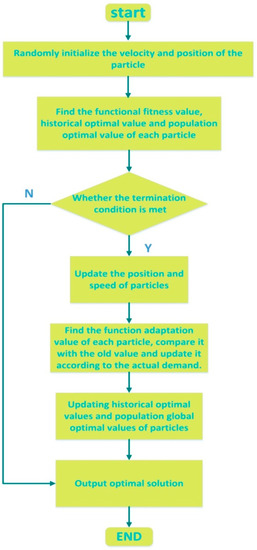
Figure 1.
Flow chart of particle swarm optimization (PSO) algorithm.
2.3.2. Particle Swarm Optimization Algorithm Optimized by Tabu Search (TS-PSO)
The traditional PSO algorithm has the advantages of easy operation and simple parameters, but it also has the disadvantages of single population, premature convergence, and easily falling into local optimal solutions. This article solved the shortcomings of traditional particle swarms by applying Tabu search tables to store the optimal and worst particles. Tabu Search is an algorithm proposed by Glover in 1986 [28]. After each search is completed, the optimal solution is marked to prevent it from falling into the local optimum. At present, many scholars have further studied it and introduced TS into the PSO algorithm.
The flow of the TS-PSO algorithm is as follows:
- Initializing the speed and position of the particle.
- The initial particle swarm is divided into two subgroups, and the class-free scaled network model is used to calculate the fitness value of each particle, then the better particles of the two subgroups are compared.
- Updating the particle velocity and position according to Formula (16).
- Assume that after R iterations, the worst and best particle adaptation values are substantially unchanged. The position of the optimal particle is stored as the current best position in the local contraindication table (Table 1), and the position of the worst particle is stored in Table 2 as the current worst position .
 Table 1. Comparison of parameter settings for various models.
 Table 2. Comparison between robust principal component analysis (RPCA) and principal component analysis (PCA).
 - Repeat steps 3 and 4.
- Determine whether the termination condition is met, and exit if it is satisfied, otherwise return to the second step.
2.4. Least Squares Support Vector Machine Optimized by the TS-PSO Algorithm
The parameter of regularization and the width of the radial basis function should be determined before using the Least Squares Support Vector Machine with RBF kernel function to forecast energy consumption. In this article, the TS-PSO algorithm was used to optimize the parameters of LSSVM. The steps are as follows:
- (1)
- Perform TS-PSO algorithm steps 1–6.
- (2)
- Assign the optimized parameters to Least Squares Support Vector Machine for constructing the forecasting model.
The flowchart of Least Squares Support Vector Machine Optimized by TS-PSO Algorithm (TS-PSO-LSSVM) is shown in Figure 2.
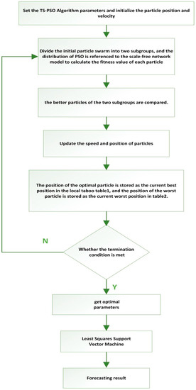
Figure 2.
The flow chart of Least Squares Support Vector Machine Optimized by TS-PSO Algorithm.
According to the above analysis, the difference between the parameter settings of TS-PSO-LSSVM and PSO-LSSVM, LSSVM, and other traditional forecasting models can be clarified, as shown in Table 1.
2.5. The Forecasting Model Based on Robust Principal Component Analysis and Least Squares Support Vector Machine Optimized by TS-PSO Algorithm (RPCA-TS-PSO-LSSVM)
Energy consumption is influenced by a multitude of direct or indirect factors. We firstly selected the GDP, population, industrial structure and energy consumption structure, and urbanization as the main affecting factors according to RPCA, which can improve data availability and forecasting accuracy. Then, we proposed the RPCA-TS-PSO-LSSVM forecasting model to forecast the energy consumption of China. The prediction process is shown in Figure 3:
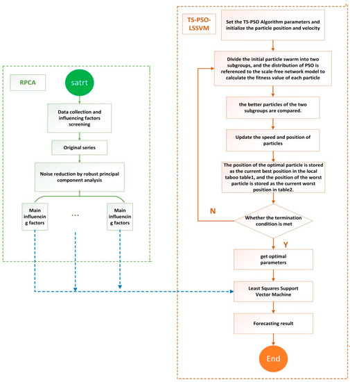
Figure 3.
The forecasting process based on the RPCA-TS-PSO-LSSVM (Robust Principal Component Analysis and PSO-LSSVM Optimized by the Tabu Search) model.
3. Empirical Analysis
3.1. Screening of Influencing Factors for Model Input
According to the literature study and China Statistical Yearbook, we selected GDP, population, industrial structure and energy consumption structure, energy intensity, total imports and exports, fixed asset investment, energy efficiency, urbanization, the level of consumption, and fixed investment in the energy industry as a set to input into the RPCA model to achieve hierarchical clustering.
3.2. Data Preprocessing
Because the scale of the experimental test data is not uniform, directly classifying according to the RPCA algorithm will result in unsatisfactory classification. The obtained raw data must be preprocessed to eliminate the non-uniformity of dimension and scale. The preprocessing method adopted in this article is a normalization method commonly used in clustering algorithms to scale the data to a small range. According to the meaning of the diagonal element representation of the covariance matrix, the data is averaged, and the difference in the degree of change of each variable can be reflected by the diagonal elements of the covariance matrix, and the original data is averaged and the variables are inter-variable. Meanwhile, the relevance of the data still exists.
Among them, is the mean, is the normalized sample data.
3.3. Hierarchical Clustering according to RPCA
In this article, the cumulative contribution rate of the main components of the two-dimensional data was compared and is shown in Table 2.
It can be concluded from the above analysis that the traditional PCA algorithm can’t effectively classify the test data, indicating that the correlation between the samples is not high, and the first two principal elements selected are not representative. The RPCA algorithm is obviously superior to traditional PCA, and the classification effect is more accurate. The comprehensive preservation of the original sample information can comprehensively represent the main information of the sample and solve the information loss problem.
After RPCA clustering, the contribution rates of affecting factors are shown in Table 3.

Table 3.
The contribution rates of affecting factors.
According to the above, a scree plot of the influencing factors is shown in Figure 4.
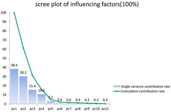
Figure 4.
Scree plot of the influencing factors.
According to the RPCA analysis results, GDP, population, industrial structure, energy consumption structure, and urbanization rate are the main components of energy consumption which are representative of the sample information. Based on the China National Statistical Yearbook, the data of the above influencing factors of 1996 to 2016 are normalized and shown in Table 4.

Table 4.
The main factors’ normalized results.
3.4. Forecasting Energy Consumption in China Based on TS-PSO-LSSVM Model
We used the outputs of the RPCA analysis as the input for three types of forecasting models. In the models, the data of 1996–2009 were used as the training set and the data of 2010–2016 were used as the test set. In order to verify that the TS-PSO-LSSVM model has high prediction accuracy, we also inputted the sample data into the traditional LSSVM and PSO-LSSVM algorithms. The forecasting results are shown in Figure 5.
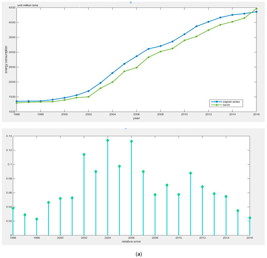
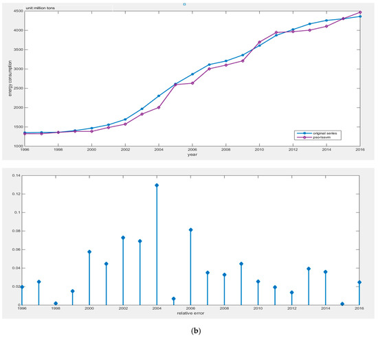
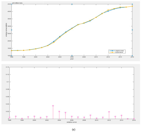
Figure 5.
Comparison of the three forecasting models: (a) forecasting results of LSSVM model; (b) forecasting result of PSO-LSSVM model; (c) forecasting result of TS-PSO-LSSVM model.
The correlation error (RE) of the three forecasting results are shown in Table 5.

Table 5.
Correlation error (RE) of three forecasting results.
In order to objectively compare the accuracy of three models, statistical indicators including RMSE, r2, and MRE were adopted in the article and the index calculation formula was as follows:
where is a real value, is a predicted value, is a sample mean, n is a sample number.
The calculation results of objectively three forecasting models are compared in Table 6.

Table 6.
The calculation results of the three models.
Furthermore, boxplots of the results are shown in Figure 6.
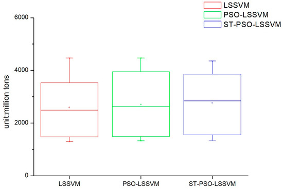
Figure 6.
Boxplots of the three forecasting models’ results.
Through the analysis of the results in Figure 5 and Figure 6 and Table 5 and Table 6, we can find that the TS-PSO-LSSVM forecasting model has higher prediction accuracy from different directions. Based on relative error, the TS-PSO-LSSVM forecasting model not only maintains a relatively low relative error, but also has a small dispersion between relative errors, which shows a high degree of stability. From the perspective of mathematical statistics, we find that TS-PSO-LSSVM< PSO-LSSVM <LSSVM from the perspective of RMSE, which indicates the TS-PSO-LSSVM model in this article has the best performance from the perspective of degree of dispersion. The prediction results have higher robustness, which can also be proved by the boxplots shown in Figure 6; TS-PSO-LSSVM> PSO-LSSVM > LSSVM from the perspective of r2 indicator; TS-PSO-LSSVM < PSO-LSSVM < LSSVM from the perspective of MRE indicator, these two indicators jointly illustrate that the proposed TS-PSO-LSSVM model has higher prediction accuracy.
Another important indicator for comparing the superiority of machine learning algorithms is the training time of the model. The shorter the training time, the higher the calculation speed, and the superiority of the algorithm can be reflected when a large amount of data is encountered. This article compared the training time of the three forecasting models, as shown in Table 7.

Table 7.
Training times of the three forecasting models.
By comparison, we can find that TS-PSO-LSSVM algorithm proposed in this article reduces the number of repetitive process executions of the PSO algorithm which needs select the optimal position and the poor position, and takes up less resources. Thus, the algorithm enables faster training speeds. At the same time, the accuracy comparison of the forecasting model has also proved that the forecasting model proposed in this article will not fall into the local optimum. Therefore, the superiority of the proposed combination algorithm is proved from the perspective of both accuracy and operation speed.
3.5. Forecasting Results
We applied GM (1, 1) (grey prediction theory) to forecast the GDP, population, industrial structure, energy consumption structure, and urbanization rate from 2017 to 2030, which was used as the input data of the TS-PSO-LSSVM forecasting model. Finally, we calculated the amount of energy consumption from 2017 to 2030, which is shown in Figure 7.
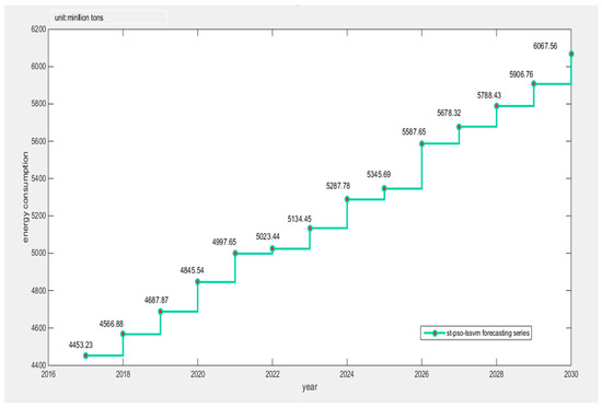
Figure 7.
The forecasting results of energy consumption from 2017 to 2030 in China.
4. Conclusions
This article combined the Tabu search algorithm with the PSO-LSSVM algorithm to construct the TS-PSO-LSSVM forecasting model for prediction of China’s energy consumption. Because the study of energy consumption is a complex issue and energy consumption is influenced by a multitude of factors, we adopted RPCA to select the main factors of GDP, population, industrial structure and energy consumption structure, urbanization, energy intensity, total imports and exports, fixed asset investment, energy efficiency, energy industry fixed investment, household consumption, and level of noise reduction. The main influential factors can contain information about other factors, while reducing the complexity of the studied factors. Compared with the traditional PCA, RPCA was proved to be better for generalizing information. After selecting the five main influential factors, we used data from 1996 to 2010 as the training set for the TS-PSO-LSSVM, PSO-LSSVM, and LSSVM forecasting models, and data from 2011 to 2016 as the test set. Then, we compared the results from forecasting of the test set form the perspective of both accuracy and operation speed. Finally, we applied the RPCA-TS-PSO-LSSVM forecasting model to forecast the future energy consumption of China in 2017–2030. We found that China’s energy consumption will break through 5000 million tons in 2020, and energy consumption will increase year by year, eventually reaching 6000 million tons in 2030. Our final conclusions and policy recommendations are as follows:
(1) From 2018 to 2030, China’s energy consumption shows a gradual upward trend, but the growth rate is gradually tightening. From the perspective of technological progress, this forecast proves that China’s energy efficiency will increase year by year.
(2) China’s energy consumption economy will transfer into the stage of diminishing returns around 2026. At that time, excessive energy investment will not bring about sustained GDP growth. Therefore, China should give priority to improving energy efficiency in the future, and continue to develop renewable energy technologies. Meanwhile, China needs to look for better opportunities in the energy investment field and continue to reduce pollutants and carbon emissions.
(3) China should pay more attention to the development of energy consumption terminal power for energy conservation and emissions reduction of the international community. At the same time, in the field of energy investment, China must attach importance to the development of the Belt and Road and grasp the opportunities of international cooperation in energy-based society. According to the forecasting results, the energy strategy of the next ten years must be carefully planned.
The forecasting results and corresponding conclusions drawn in this article have laid a strong foundation for our future research, especially the research hotspots of China’s carbon emission related to energy consumption and China’s investment ability in Belt and Road countries.
Author Contributions
In this research activity, all authors were involved in the data collection and preprocessing phase, model constructing, empirical research, results analysis and discussion, and manuscript preparation. All authors have approved the submitted manuscript.
Funding
This work is funded by the 2017 Special Project of Cultivation and Development of Innovation Base (No. Z171100002217024).
Acknowledgments
The completion of this paper has been helped by many teachers and classmates. We would like to express our gratitude to them for their help and guidance.
Conflicts of Interest
The authors declare no conflict of interest.
References
- BP Statistical Review of World Energy. Available online: https://www.bp.com/content/dam/bp/en/corporate/pdf/energy-economics/statistical-review/bp-stats-review-2018-full-report.pdf (accessed on 30 June 2018).
- Liang, Z. Effects of different stages of the energy consumption of urbanization factors. J. Shanghai Univ. Financ. Econ. 2010, 5, 89–96. [Google Scholar]
- Xu, S.; He, Z.; Long, R. Factors that influence carbon emissions due to energy consumption in China: Decomposition analysis using LMDI. Appl. Energy 2014, 127, 182–193. [Google Scholar] [CrossRef]
- Omri, A. CO2 emissions, energy consumption and economic growth nexus in MENA countries: Evidence from simultaneous equations models. Energy Econ. 2013, 40, 657–664. [Google Scholar] [CrossRef]
- Poumanyvong, P.; Kaneko, S. Does urbanization lead to less energy use and lower CO2 emissions? A cross-country analysis. Ecol. Econ. 2010, 70, 434–444. [Google Scholar] [CrossRef]
- Zhou, X.; Zhang, J.; Li, J. Industrial structural transformation and carbon dioxide emissions in China. Energy Policy 2013, 57, 43–51. [Google Scholar] [CrossRef]
- Meng, F.; Liu, Y.; Liu, L.; Li, Y.; Wang, F. Studies on Mathematical Models of Wet Adhesion and Lifetime Prediction of Organic Coating/Steel by Grey System Theory. Materials 2017, 10, 715. [Google Scholar] [CrossRef]
- Lee, Y.; Tong, L. Forecasting energy consumption using a grey model improved by incorporating genetic programming. Energy Convers. Manag. 2011, 52, 147–152. [Google Scholar] [CrossRef]
- Lin, C.; Liou, F.; Huang, C. Grey forecasting model for CO2 emissions: A Taiwan study. Adv. Mater. 2011, 88, 3816–3820. [Google Scholar] [CrossRef]
- Ghaedi, M.; Rahimi, M.; Ghaedi, A.M.; Tyagi, I.; Agarwal, S.; Gupt, V.K. Application of least squares support vector regression and linear multiple regression for modeling removal of methyl orange onto tin oxide nanoparticles loaded on activated carbon and activated carbon prepared from Pistacia atlantica wood. J. Colloid Interface Sci. 2016, 461, 425–434. [Google Scholar] [CrossRef]
- Sehgal, V.; Tiwari, M.K.; Chatterjee, C. Wavelet Bootstrap Multiple Linear Regression Based Hybrid Modeling. Water Resour. Manag. 2014, 10, 2793–2811. [Google Scholar] [CrossRef]
- Cogoljevic, D.; Gavrilovic, M.; Roganovic, M.; Matic, I.; Piljan, I. Analyzing of consumer price index influence on inflation by multiple linear regression. Phys. A Stat. Mech. Appl. 2018, 505, 941–944. [Google Scholar] [CrossRef]
- Yi, M.; Qiao, M.; Ying, F.; Okada, N.; Tsai, H.T. A scenario analysis of energy requirements and energy intensity for China’s rapidly developing society in the year 2020. Technol. Forecast. Soc. Chang. 2006, 73, 405–421. [Google Scholar]
- Zhu, Y.; Zheng, W.; Li, P.; Wang, L.; Zou, X. Simulation on China’s Economy and Prediction on Energy Consumption and Carbon Emission under Optimal Growth Path. Acta Geogr. Sin. 2009, 64, 935–944. [Google Scholar]
- Zhang, G.P. Time series forecasting using a hybrid ARIMA and neural network model. Neurocomputing 2003, 50, 159–175. [Google Scholar] [CrossRef]
- Erdogdu, E. Electricity demand analysis using cointegration and ARIMA modelling: A case study of Turkey. Energy Policy 2007, 35, 1129–1146. [Google Scholar] [CrossRef]
- Luong, H.V.; Deligiannis, N.; Seiler, J.; Forchhammer, S.; Kaup, A. Compressive Online Robust Principal Component Analysis via n-l1 Minimization. IEEE Trans. Image Process. 2018, 27, 4314–4329. [Google Scholar] [CrossRef] [PubMed]
- Chrétien, S.; Clarkson, P.; Garcia, M.S. Application of Robust PCA with a structured outlier matrix to topology estimation in power grids. Int. J. Electr. Power Energy Syst. 2018, 100, 559–564. [Google Scholar] [CrossRef]
- Sadeghian, A.; Wu, O.; Huang, B. Robust probabilistic principal component analysis based process modeling: Dealing with simultaneous contamination of both input and output data. J. Process. Control 2018, 67, 94–111. [Google Scholar] [CrossRef]
- Wu, M.; Sun, Y.; Hang, R.; Liu, Q.; Liu, G. Multi-component group sparse RPCA model for motion object detection under complex dynamic background. Neurocomputing 2018, 314, 120–131. [Google Scholar] [CrossRef]
- Roushangar, K.; Saghebian, S.M.; Mouaze, D. Predicting characteristics of dune bedforms using PSO-LSSVM. Int. J. Sediment Res. 2017, 32, 515–526. [Google Scholar] [CrossRef]
- Huan, J.; Cao, W.; Qin, Y. Prediction of dissolved oxygen in aquaculture based on EEMD and LSSVM optimized by the Bayesian evidence framework. Comput. Electron. Agric. 2018, 150, 257–265. [Google Scholar] [CrossRef]
- Xue, X. Evaluation of concrete compressive strength based on an improved PSO-LSSVM model. Comput. Concr. 2018, 21, 501–511. [Google Scholar]
- Lu, P.; Ye, L.; Su, B.; Zhang, C.; Zhao, Y.; Teng, J. A new hybrid prediction method of ultra-short-term wind power forecasting based on EEMD-PE and LSSVM optimized by the GSA. Energies 2018, 11, 697. [Google Scholar] [CrossRef]
- Zhao, H.; Huang, G.; Yan, N. Forecasting energy-related CO2 emissions employing a novel SSA-LSSVM model: Considering structural factors in China. Energies 2018, 11, 781. [Google Scholar] [CrossRef]
- Wen, T.; Tang, H.; Wang, Y.; Lin, C.; Xiong, C. Landslide displacement prediction using the GA-LSSVM model and time series analysis: A case study of Three Gorges Reservoir, China. Nat. Hazards Earth Syst. Sci. 2017, 17, 2181–2198. [Google Scholar] [CrossRef]
- Liu, C.; Niu, P.; Li, G.; You, X.; Ma, Y.; Zhang, W. A Hybrid Heat Rate Forecasting Model Using Optimized LSSVM Based on Improved GSA. Neural Process. Lett. 2017, 45, 299–318. [Google Scholar] [CrossRef]
- Gorjaei, R.G.; Songolzadeh, R.; Torkaman, M.; Safari, M.; Zargar, G. A novel PSO-LSSVM model for predicting liquid rate of two phase flow through wellhead chokes. J. Nat. Gas Sci. Eng. 2015, 24, 228–237. [Google Scholar] [CrossRef]
- Zhang, X. Short-Term Load Forecasting for Electric Bus Charging Stations Based on Fuzzy Clustering and Least Squares Support Vector Machine Optimized by Wolf Pack Algorithm. Energies 2018, 11, 1449. [Google Scholar] [CrossRef]
- Peng, B.; Lü, Z.; Cheng, T.C.E. A tabu search/path relinking algorithm to solve the job shop scheduling problem. Comput. Oper. Res. 2015, 53, 154–164. [Google Scholar] [CrossRef]
- Escobar, J.W.; Linfati, R.; Toth, P.; Baldoquin, M.G. A hybrid Granular Tabu Search algorithm for the Multi-Depot Vehicle Routing Problem. J. Heuristics 2014, 20, 483–509. [Google Scholar] [CrossRef]
- Li, X.; Gao, L. An effective hybrid genetic algorithm and tabu search for flexible job shop scheduling problem. Int. J. Prod. Econ. 2016, 174, 93–110. [Google Scholar] [CrossRef]
- Sicilia, J.A.; Quemada, C.; Royo, B.; Escuín, D. An optimization algorithm for solving the rich vehicle routing problem based on Variable Neighborhood Search and Tabu Search metaheuristic. J. Comput. Appl. Math. 2016, 291, 468–477. [Google Scholar] [CrossRef]
- Wright, J.; Ma, Y.; Candes, E.J.; Li, X. Robust Principal Component Analysis? J. ACM 2011, 58, 11. [Google Scholar]
- Lin, Z.; Chen, M.; Ma, Y. The Augmented Lagrange Multiplier Method for Exact Recovery of Corrupted Low-Rank Matrices. Available online: https://arxiv.org/pdf/1009.5055.pdf (accessed on 2 June 2018).
© 2019 by the authors. Licensee MDPI, Basel, Switzerland. This article is an open access article distributed under the terms and conditions of the Creative Commons Attribution (CC BY) license (http://creativecommons.org/licenses/by/4.0/).