State of Charge Estimation for Lithium-Bismuth Liquid Metal Batteries

Abstract

Lithium-bismuth liquid metal batteries have much potential for stationary energy storage applications, with characteristics such as a large capacity, high energy density, low cost, long life-span and an ability for high current charge and discharge. However, there are no publications on battery management systems or state-of-charge (SoC) estimation methods, designed specifically for these devices. In this paper, we introduce the properties of lithium-bismuth liquid metal batteries. In analyzing the difficulties of traditional SoC estimation techniques for these devices, we establish an equivalent circuit network model of a battery and evaluate three SoC estimation algorithms (the extended Kalman filter, the unscented Kalman filter and the particle filter), using constant current discharge, pulse discharge and hybrid pulse (containing charging and discharging processes) profiles. The results of experiments performed using the equivalent circuit battery model show that the unscented Kalman filter gives the most robust and accurate performance, with the least convergence time and an acceptable computation time, especially in hybrid pulse current tests. The time spent on one estimation with the three algorithms are 0.26 ms, 0.5 ms and 1.5 ms.

1. Introduction

The use of energy storage systems could significantly improve the reliability and efficiency of power grids, with respect to the integration of intermittent renewable energy sources [1]. At present, the limitation on the widespread application of batteries is their high cost. Liquid metal batteries (LMBs) have the potential to meet the requirements for stationary energy storage applications [2,3], since in addition to the low cost of a single cell, these devices have a large capacity and a long service life, compared with the more widely used lithium-ion batteries and lead-acid batteries. The measured capacity loss after operation for more than 450 charge–discharge cycles at 100 percent depth of discharge with the current densities as 1000 milliamperes per square centimeter, projects retention of over 85 percent of initial capacity after ten years of daily cycling [2]. As well as their increased energy density, these characteristics are advantageous in reducing the cost of adoption of LMBs, particularly for large-scale applications. However, commercialization has not been realized because of the initial limitations of LMB technology. Early LMB devices used magnesium and antimony as cathodes and anodes, respectively and MgCl₂-KCl-NaCl, a mixed molten salt, as an electrolyte, leading to a working voltage of approximately 0.4 V and a high operational temperature of 700 °C [4]. In recent years, considerable effort has been put into the selection of high performance electrodes, electrolytes to improve their working voltage and reduce their operational temperature and sealants capable of effective heat insulation at high temperatures over long periods of time. The life cycle and failure mechanisms of these cells have also been studied, resulting in improved understanding of how to make this technology more viable. Based on this research, a new type of LMB, consisting of lithium and bismuth, has been proposed [5,6,7], with commercial cells produced by the Xi’an Jiaotong University in China. This device could be charged or discharged at a high rate of capacity for a long time without any irreversible damage, which means it could deal with larger current fluctuations. Also, the hysteresis effect can be ignored and no safety problems will be caused by overcharge and over discharge. However, the operational temperature of this device needs to be maintained at 500 °C, to ensure that the LiCl-LiF electrolyte remains in a molten state and the working voltage of the device is 0.7 V, which is relatively low [7]. Although these cells do not fulfil every requirement for grid-level energy storage, their development has created the opportunity for practical application-oriented research.

An additional consideration for large-scale energy storage systems is the inclusion of a battery management system (BMS), which typically monitors the state of charge (SoC) of a battery [8,9]. This parameter is defined as the remaining usable capacity of a device. Accurate estimation of the SoC is required to avoid over-charging or over-discharging, which degrade the cell and to give the user a clear indication of the working time of the battery. Hence, BMSs are required to maximize the improvements in performance gained as a result of the development of Li-Bi LMBs.

There have been many studies on SoC estimation techniques. From these, the most reliable method has proven to be the discharge test. However, this technique is time-consuming and impractical for on-line estimation. In contrast, the simplest estimation method is Coulombic counting, a technique which is widely used in most consumer applications [10]. As the SoC and open circuit voltage (OCV) of a battery are related, this metric can also be used for SoC estimation. However, the accuracy of this method is limited and, consequently, it is typically used in combination with other techniques [11,12,13,14,15,16]. A range of data driven estimation methods have been increasingly studied, because, unlike techniques such as OCV, exact knowledge of the behavior of a battery is not required for accurate estimation. Such methods include, support vector machines [17,18,19], the combined grey model and genetic algorithm approach developed by Chen et al. [20] and the fuzzy logic-based estimator for Li-ion batteries developed by Singh et al. [21]. In spite of these developments, data-driven methods feature time-consuming computation and require large amounts of data training [22]. Hence, model-based estimation methods have been developed as a way to determine the SoC of a battery using its current performance, by relating this to a model system, which is typically non-linear.

Additional signal processing is required when model-based estimation techniques are used to determine a battery’s SoC. Modified Kalman filters are often employed for this purpose, which include processing steps to address the non-linear system. For instance, an extended Kalman filter was adopted [23,24] to linearize the battery model. Other efforts have been made to reduce non-convergence and improve the speed of convergence [25,26]. Sigma-point Kalman filters, such as the unscented and central-difference Kalman filters, have been studied, for better consideration of model nonlinearities [27], while Liu et al. applied an extended fractional Kalman filter to a fractional order battery model, in consideration of non-linear effects [28]. Although they have proven useful, Kalman filters are limited, in that they are optimized for operation with noise with a Gaussian probability density. In contrast, by describing the probability density function as a set of particles using Monte Carlo sampling methods, the particle filter is able to consider any probability distribution [29], suggesting that it is a more universal alternative to Kalman filters.

Recent research has demonstrated that more accurate SoC estimation can be achieved using multiple-model techniques, which combine the estimates of different models [30,31,32] or treat the result derived from one model as the initial constraint [33,34,35,36] of another model. These can be a combination of all model-based methods [37], data-driven methods and model-based methods [38] or some other flexible combination [39]. Tran N T et al. explored a method combining dual extended Kalman filters with auto regressive exogenous on-line parameter estimation, for SoC and state of health estimation [39], while Li Y et al. used recursive Bayesian filtering for SoC estimation based on the features obtained from a Markov model [40].

Most of the techniques listed above were studied for Li-ion and lead-acid batteries. The application of these methods to devices such as lithium-sulphur batteries has also been explored [41,42]. However, to date, they have not been applied to Li-Bi LMBs, a fact that can be explained by the differences between them and Li-ion batteries. For instance, the characteristic OCV-SoC curves of the latter device enables SoC estimation, as their variation is generally monotonic. In contrast, the variation of the OCV of an LMB, with respect to SoC, is minimal in a wide range of operation. These devices also have a low operating voltage of about 0.7 V, which increases the difficulty in resolving changes in voltage. In addition, the polarization voltage parameters of LMBs differ from those of Li-ion batteries, due to their unique working principles. Finally, the Coulombic and energy efficiencies of these batteries are sensitive to the applied current profile, while their rated current is about 50 A, far greater than it is for Li-ion batteries. Until recently, few SoC estimation methods for Li-Bi batteries had been published. In this paper, we evaluate three SoC estimation techniques using an equivalent circuit network model of a Li-Bi LMB, to verify their applicability to this technology.

The rest of this paper is organized as follows: Li-Bi LMBs are introduced in Section 2. Then description of the experimental setup and the practical test conducted on the cell is included in Section 3, in addition to the equivalent circuit model used in SoC estimation and the parameter identification system. A discussion on conventional techniques used in SoC estimation and limitations on their application to Li-Bi LMBs is included in Section 4. In this discussion, we consider the extended Kalman filter, the unscented Kalman filter and the particle filter. The results of simulations using these algorithms and evaluation of their performance, are reported in Section 5. The paper concludes with a discussion on the applicability of these techniques to Li-Bi LMBs in Section 6.

The main contribution of this paper is the development and evaluation of three recursive SoC estimators for liquid metal batteries as a foundation for the future study on battery management for these devices. To the best of the authors’ knowledge, no similar work has appeared elsewhere in the literature.

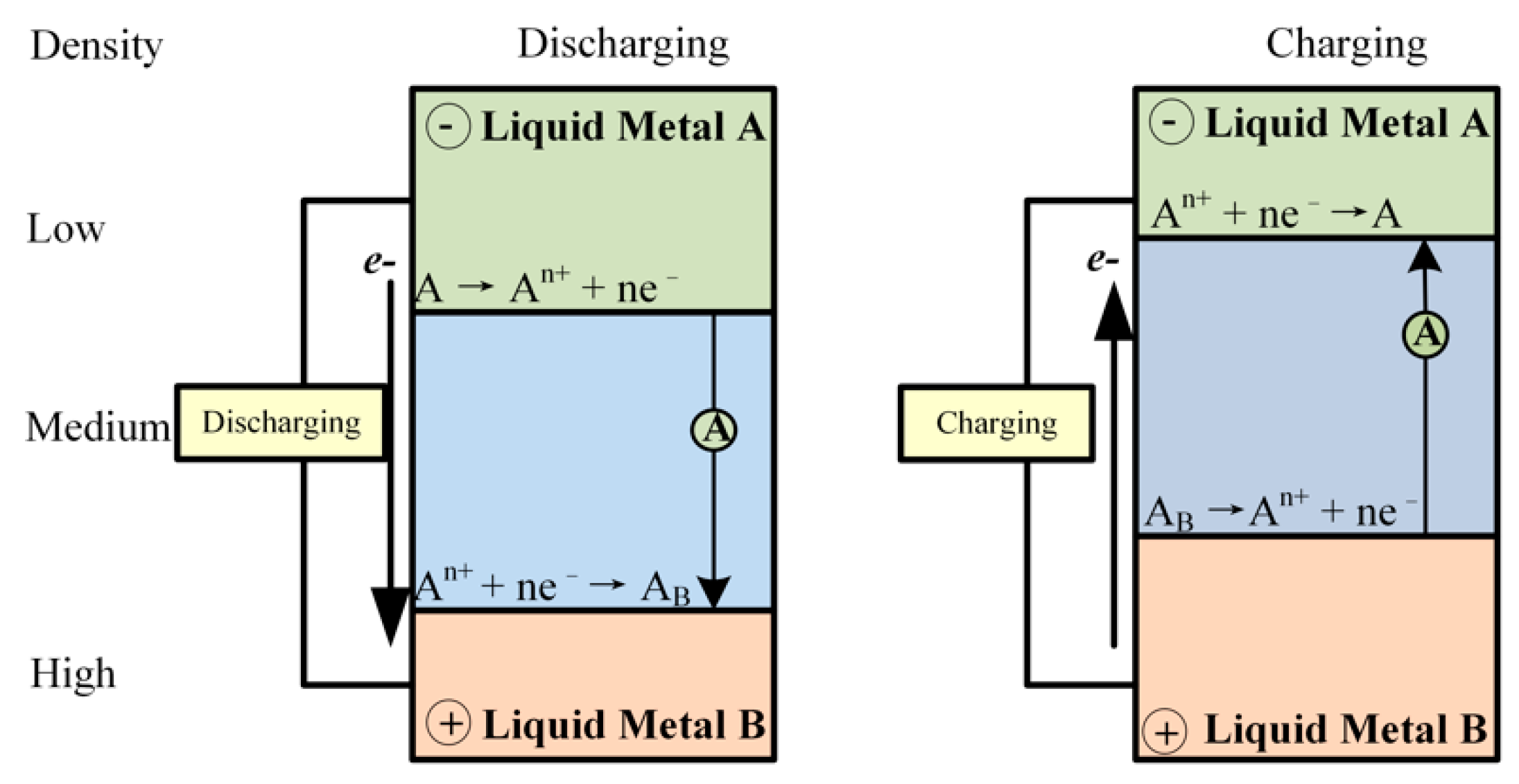
2. Lithium-Bismuth Liquid Metal Battery

Li-Bi LMBs consist of a negative lithium metal electrode, a positive bismuth metal electrode and a LiCl-LiF molten salt electrolyte [6]. Since molten metals and molten salts are immiscible, they automatically stratify, due to their differing densities, as shown in Figure 1. This self-stratification removes the requirement for special battery separators, which reduces the cost of a battery and enables battery systems to be enlarged and produced more easily [2,7].

The use of liquid electrodes means that solid-state degradation mechanisms, such as dendrimer growth and fracture, can be avoided, which are the main causes of failure in other battery technologies. During discharge, lithium is oxidized to lithium-ions at the negative electrode. These ions are dissolved into the electrolyte, which subsequently releases electrons into the terminal circuit. At the same time, lithium-ions in the electrolyte are reduced to lithium metal at the positive electrode, which then alloys with bismuth [7]. This process stops when the voltage drops below the defined cut-off voltage or when the battery reaches the desired depth of discharge. These reactions are reversed when the battery is charged. The most remarkable merit of Li-Bi LMBs is that they can be charged or discharged at a high rate of capacity, for a long time, without any damage [7]. In addition, the hysteresis effect often observed with voltage can be ignored. The operational temperature of this device needs to be maintained at 500 °C, to ensure that the LiCl-LiF electrolyte remains in a molten state.

The main parameters of a Li-Bi LMB are summarized in

Table 1. Parameters of a Li-Bi liquid metal battery.

Nominal capacity	200 Ah
Nominal voltage	0.7 V
Cut-off voltage (charging, discharging)	1.2 V, 0.4 V
Self-discharge current	0.4 A
Rated working current	50 A (0.25 C)
Operating temperature	500 °C
Weight	4.8 kg
Size (diameter, height)	18 cm, 10 cm
Cost	240 $ kWh−1 [7]

. We note that when the SoC ranges between 0% and 65%, there is little variation in OCV and the curve is effectively a horizontal line. In addition, unlike Li-ion and other solid-state batteries, the internal resistance of LMBs is affected by the internal temperature and effective thickness of the electrolyte layer, which changes with the battery’s state of operation.

As this Li-Bi LMB is intended for use in power grids, as compensation for renewable energy sources such as wind power, the battery will switch frequently between charging, discharging and static modes of operation, which means the working current of the battery also fluctuates frequently. The unique proprieties of LMBs means that precise estimation of the SoC is required for protecting the device from overcharging or discharging, offering reference for the capacity equilibrium of battery packs and showing the residual capacity and the remaining working time to users. Careful monitoring is particularly necessary for SoCs between 0% and 65%.

3. Experimental Details and Equivalent Circuit Model

In this section, we describe the experimental setup and the details of the current profiles used in this paper, as well as establish the equivalent circuit model for the LMB. Finally, the relationship between the parameters derived in this model and SoC are also determined.

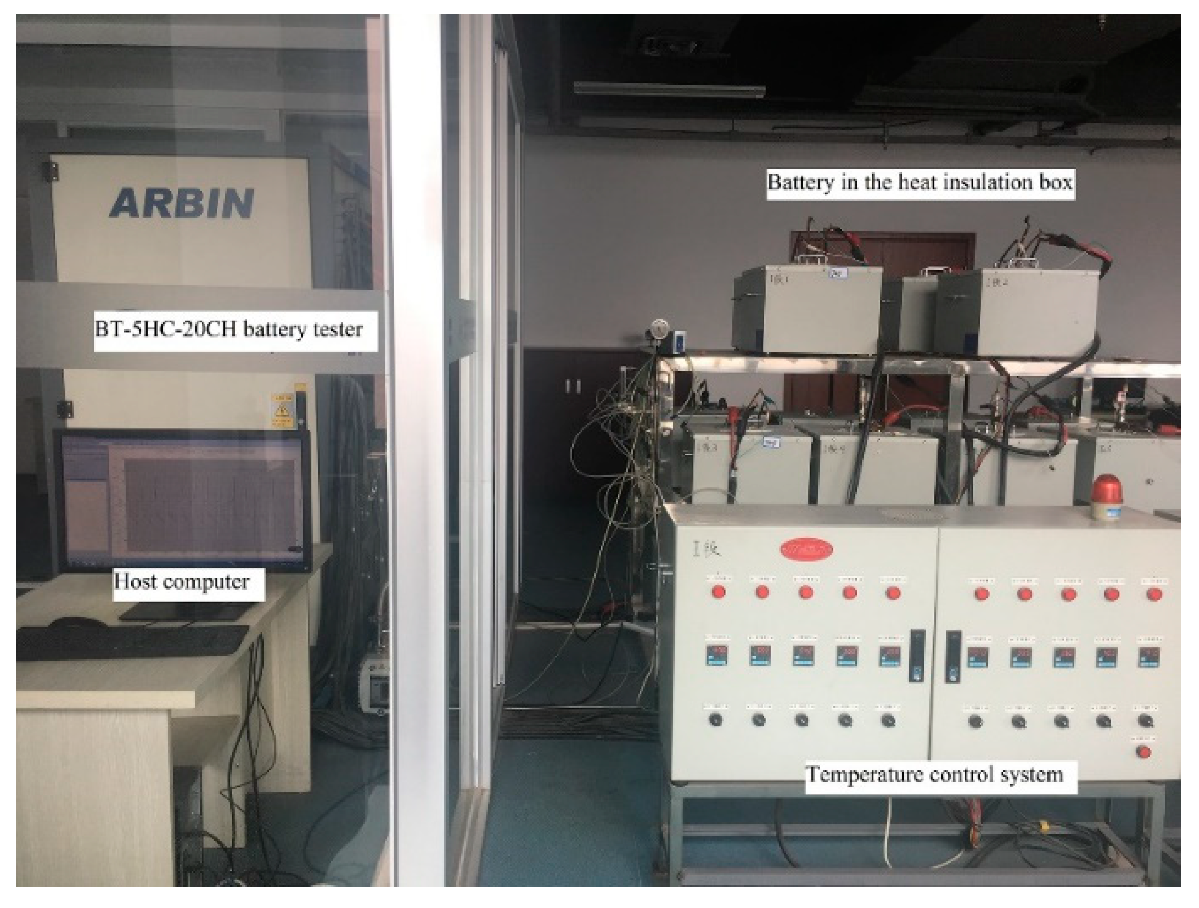
3.1. Experiment Details

Experiments were conducted on a Li-Bi LMB, to generate a dataset for verification of parameter identification based on battery modelling and the proposed SoC estimation methods. The experimental set up, consisting of a Li-Bi LMB, battery tester, temperature control system, holding furnace and a host computer, is shown in Figure 2. Tests were conducted at room temperature, while the combination of the temperature control system and the heat insulation box maintained the cell at 500 °C. Current profiles for experimentation were designed on the host computer and loaded on the test cell using the BT-5HC-20CH battery testing system produced by ARBIN Instruments. The measurement ranges of this device are −100–100 A for current and 0–5 V for voltage, with a precision of ±0.02% FSR, for both types of measurement. This error is small enough to enable the assumption that parameters estimated using these measurements are their actual value. The testing system records a range of information, including date, time, cycle index, current, voltage, charge capacity, discharge capacity, charge energy and discharge energy. In these experiments, SoC was determined using the charge and discharge capacity. Data acquired by the battery tester was transmitted to the host computer, on which it was stored, over TCP/IP.

A depiction of the four current profiles obtained during testing is shown in Figure 3. Datasets comprising current, charge capacity, discharge capacity, terminal voltage and experiment duration, were obtained for each profile, which were subsequently used for identification of the parameters of the battery model, for evaluation of the proposed models.

Prior to experimentation, we allowed the cell to rest in a state of complete charge or discharge (depending on the current profile being recorded) for 12 h, for equilibration. The initial state of the cell was then recorded as the initial OCV. For acquiring the pulsed current profile, we applied 50 pulses of −50 A, resting 40 min after each pulse, until the charge cut-off voltage (1.2 V) was reached, as shown in Figure 3a. The pulse-width in this process was 20 min. The OCV of the cell was measured during the rest periods, for characterization of its relationship to SoC. Similarly, for the pulsed discharge profile, 50 pulses of 50 A were applied, until the discharge cut-off voltage (0.4 V) was reached, as shown in Figure 3b. The pulse-width in this process was also 20 min. The OCV in this curve is the mean of the OCVs measured during the pulse charge and pulse discharge processes.

The constant current discharge profile shown in Figure 3c was obtained by applying a current of 50 A to the cell, until the cut-off voltage was reached. Finally, to consider a more realistic scenario [43], we obtained the hybrid pulse current profile shown in Figure 3d. In this experiment, a current was randomly selected from the −0.4 C (−80 A) to 0.4 C (80 A) range, spaced at a multiple of 0.025 C intervals and applied to the cell. Current selection and modification were repeated every 60 s, for the duration of the experiment. The enlarged plots in the insets of Figure 3d highlight the details of the current profile and the corresponding changes in voltage and SoC.

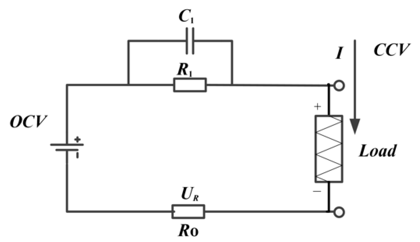
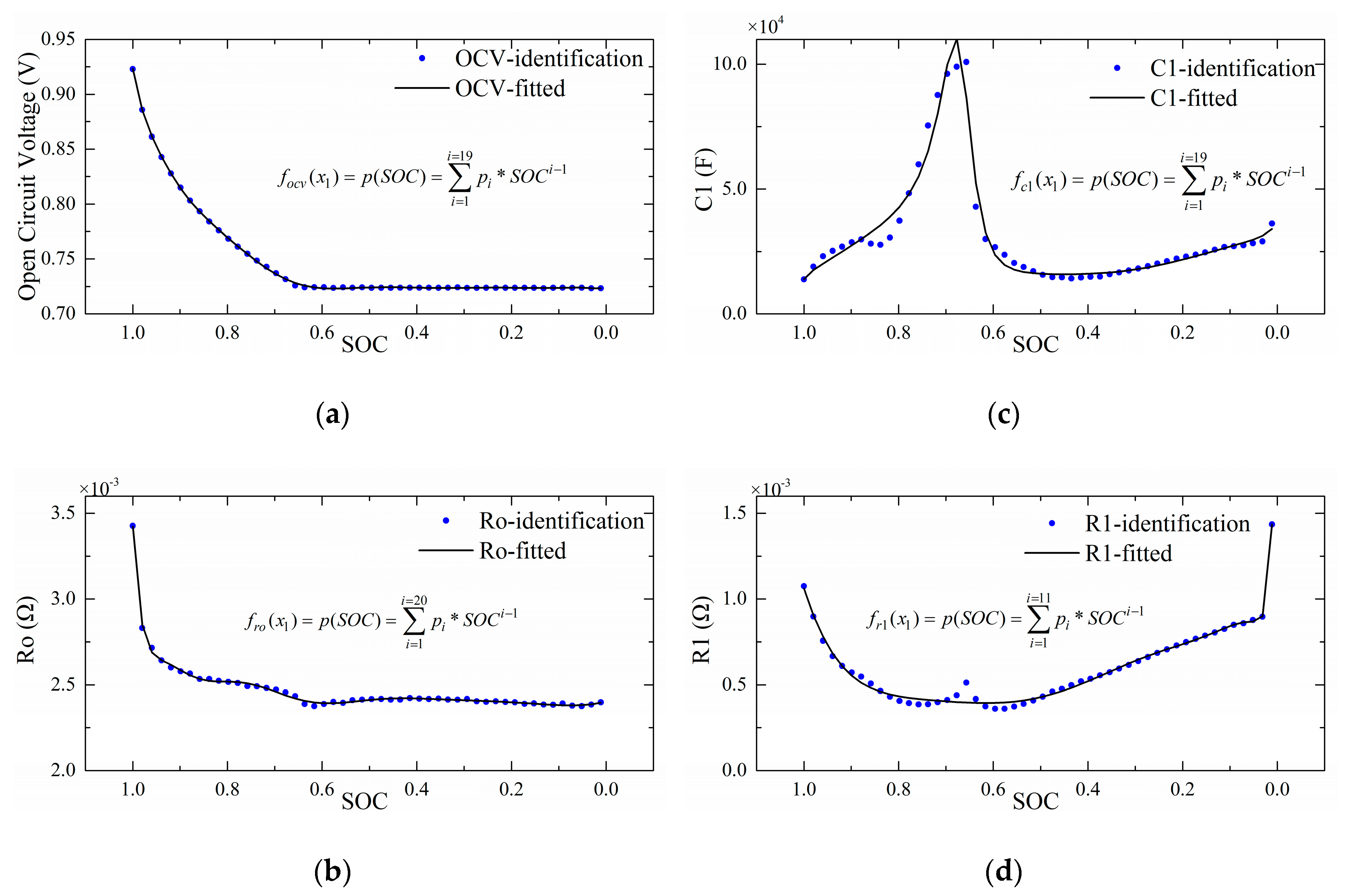
3.2. Equivalent Circuit Model and Parameter Identification

The equivalent circuit of the LMB [44] used in this paper, a first-order Thevenin model, is shown in Figure 4. The model consists of a first- order parallel resistor-capacitor (R₁ and C₁) network, an internal resistance (R_o) and an open circuit voltage (OCV). The closed-circuit voltage (CCV) is defined as the voltage across the load, consisting of a polarization voltage (u_p), OCV and an internal resistance voltage (U_R). The current (I) is assumed to be positive in the discharge direction. Self-discharge is ignored as it is a long-term cumulative effect, with little influence on the transient response of the device.

To describe the battery model used in estimation, functions relating OCV, R_o, R₁, C₁ and SoC are essential. The relationships between OCV and SoC during charge and discharge processes were obtained using the datasets depicted in Figure 3a,b. An OCV-SoC curve can be drawn by taking the mean of the OCV values obtained from the two different processes, as shown in Figure 5a, which enables parameter identification.

The relationships between R_o, R₁, C₁ and SoC can be determined by first considering how the former three values are defined in the battery model established in Figure 4. R_o is defined as in (1), below, where ΔU and ΔI are the instantaneous change in voltage and current caused by variations to the current profile.

$$R_{\mathrm{o}}=\Delta U/\Delta I$$

(1)

The values of ΔU and ΔI at different SoCs were obtained from the dataset depicted in Figure 3b, enabling us to plot the R_o-SoC curve displayed in Figure 5b.

Using the measured CCV-SoC curve and the estimated OCV-SoC and R_o-SoC curves, the relationship between u_p and SoC can be defined as in (2) and the relationship between u_p, R₁ and C₁ can be defined as in (3). The relationship between R₁, C₁ and SoC can thus be determined from these equations. The curves depicting these relationships are shown in Figure 5c,d.

$$CCV=OCV-U_{\mathrm{p}}-I{R}_{\mathrm{o}}$$

(2)

$$\frac{\mathrm{d}{u}_{\mathrm{p}}}{\mathrm{d}t}=-\frac{u_{\mathrm{p}}}{C_1{R}_1}+\frac{I}{C_1}$$

(3)

We fit polynomial functions to these curves, with parameters determined using the Levenberg-Marquardt algorithm [45]. The curves depicting these relationships are shown in Figure 5.

Equations (A1)–(A4) in Appendix A express the mathematical relationships depicted in the OCV-SoC, R_o-SoC, C₁-SoC and R₁-SoC curves, respectively.

The state-space model of the cell is established as in Equations (4) and (5), where x~[SoC, u_p]^T represents the state of the system and y = [OCV] represents the output of the system. x₁ and x₂ are the first and second row of x (i.e., SoC and u_p) respectively and Q_m is the rated capacity of the cell.

$$x_k=\left[\begin{array}{c}So{C}_k\\ u_{p,k}\end{array}\right]=\left[\begin{array}{cc}1& 0\\ 0& 1-\frac{1}{f_{c1}(x_{1,k-1})f_{r1}(x_{1,k-1})}\end{array}\right]x_{k-1}+\left[\begin{array}{c}\frac{-1}{3600{\mathrm{Q}}_{\mathrm{m}}}\\ \frac{1}{f_{c1}(x_{1,k-1})}\end{array}\right]I_k$$

(4)

$$y_{\mathrm{k}}=f_{ocv}(x_{1,\mathrm{k}})-x_{2,\mathrm{k}}-I_{\mathrm{k}}{f}_{ro}(x_{1,\mathrm{k}})$$

(5)

4. SoC Estimation Algorithms

In this section, we explain the reasons behind the selection of the algorithms used in testing, by discussing the characteristics of SoC estimation techniques in relation to the properties of Li-Bi LMBs.

4.1. Applicability of Traditional Techniques

4.1.1. Open Circuit Voltage Method

Studies have shown that the electromotive force and by extension, the open circuit voltage of lead-acid and Li-ion batteries, is closely related to their SoC. The relationship between these values enables OCV to be used for SoC estimation. Although in some cases, such as with MH/Ni and Li-ion batteries, the relationship between these two parameters is not strictly linear, a simple mathematical equivalence relating OCV and SoC can typically be found. Despite its arguable accuracy, this method is widely used, as it is the simplest and fastest SoC estimation technique [22]. However, as OCV can only be measured accurately when a battery is in a stable state, this technique is not suitable for on-line monitoring, as devices frequently transition between charging and discharging process, without enough time for stabilization. As the OCV-SoC curve of an LMB is practically static when the SoC is between 0% and 65%, this technique is not suitable for these devices.

4.1.2. Ampere Hour Counting Method

Ampere hour (Ah) counting, also known as the Coulombic counting method, is the most-widely used SoC estimation technique in BMSs. With this method, SoC is estimated by continuously monitoring the dissipated current and the duration of operation. Assuming the capacity of the battery is known, this information can be used to calculate the SoC, by subtracting the discharged capacity from the initial value, which is typically determined using the open circuit voltage method [10]. In spite of its adoption, this method has several shortcomings. For instance, integration and accumulation errors are difficult to eliminate. The degradation of battery capacity, caused by factors such as working temperature, aging and discharging current and changes to cell capacity, caused by fluctuating currents, intensify errors in SoC estimation. This method is not practical for use with LMBs because determining their initial SoC is difficult. In addition, these devices are intended for compensation for intermittent energy sources, in which the working current fluctuates in a wide range.

4.1.3. Data-Driven Methodology

Extensive study has been conducted on data driven estimation methods, because of their flexibility and model-free characteristic. These methods are typically used as a black-box, taking some measurable and representative factors associated with a battery’s SoC, such as open circuit voltage, internal resistance and temperature, as an input for calculation to get the required information. While many implementations of this methodology exist, such as the evolutionary algorithm, support vector machines [19], genetic algorithms [20] and fuzzy logic [21], most of the parameters used when these algorithms have been applied with Li-ion batteries do not have similar analogues in LMBs. Thus, the relationships required for estimation are more complex and there is no record that these techniques have been used for Li-Bi LMBs, as a result.

4.1.4. Model-Based Methods

As the name suggests, with model-based methods, equivalent circuit network (ECN) or battery models, such as the pure resistance ECN model, Thevenin ECN model [46], general non-linear model (GNL) and the new generation of American car partnership plan (PNGV) [47] are defined, to describe the behavior of a battery. State machines of these models are subsequently established, which predict terminal voltage as the output of the system. The core idea of these methods is to produce the optimal estimate of the terminal voltage of the battery, with minimum variance, by reducing the error between the predicted and measured values, using recursive algorithms. A compromise is required between the complexity of the ECN model and the selected algorithm, to ensure it can be processed in the BMS. ECN models which combine the open circuit voltage method with Ah counting may provide the possibility of SoC estimation for Li-Bi LMB. Although recursive algorithms such as particle filter [35], particle swam optimization [48,49], least squares methods [50] and Kalman filter-based methods (e.g., the extended Kalman filter [23], unscented Kalman filter [27] and adaptive unscented Kalman filter [51] algorithms) can be considered implementations of this technique, no record of their application with Li-Bi LMBs exists in the literature.

The unique properties of LMBs suggest that filters are the most suitable option for SoC estimation for these devices, as the large number of iterative processes can reduce the estimation error, caused by fluctuating working current and the quasi-static relationship between working voltage and SoC and eliminate the influence of the initial SoC, which can be difficult to determine for LMBs. To explore this possibility, three algorithms are discussed and evaluated: the extended Kalman filter (EKF), the unscented Kalman filter (UKF) and the particle filter (PF).

4.2. Extended Kalman Filter

In the context of this paper, the Kalman filter (KF) is used to provide an optimal estimate of the SoC of a system from observation data. As this data is affected by noise and interference, estimation is effectively a filtering process. To complete this, a linear model describing the relationship between the input and output of the system is first established. However, as the ECN model of LMB is non-linear, as established in Section 3.2, intermediate steps are needed to convert this system into a form suitable for processing with the KF. In the EKF, these intermediate steps are implemented by converting the nonlinear system into an approximate linear system using a first order Taylor series expansion centered on a reference value [23]. The non-linear state-space model used in this study is shown in Equations (4) and (5). The operation of this algorithm is summarized in

Table 2. Summary of extended Kalman filter operation [23].

Non-linear state-space model and linearized model $\{\begin{array}{l}{x}_k=f(x_{k-1},i_{k-1},{\omega }_{k-1},k-1)\\ y_k=g(x_k,i_k,{\upsilon }_k,k-1)\end{array}\{\begin{array}{l}{\stackrel{⌢}{x}}_k^{-}\approx {\stackrel{⌢}{A}}_{k-1}^{-}{\stackrel{⌢}{x}}_{k-1}^{+}+{\stackrel{⌢}{B}}_{k-1}^{-}{\overline{\omega }}_{k-1}\\ {\stackrel{⌢}{y}}_k\approx g({\stackrel{⌢}{x}}_k^{-},i_k,{\overline{\upsilon }}_k,k)\end{array}$

Step 1: Initialization ${\widehat{x}}_0^{+}=E(x_0),P_0=\mathrm{E}\left[(x_0-{\widehat{x}}_0^{+}\left)\right(x_0-{\widehat{x}}_0^{+}{)}^{\mathrm{T}}\right],Q=\mathrm{E}(\omega {\omega }^T),R=\mathrm{E}(\upsilon {\upsilon }^T)$

For k = 1, 2, ..., n, loop from step 2 to step 10. Step 2: Update Jacobian matrices: Ak, Bk, $A_k={\frac{\partial f(x_k,i_k,{\omega }_k,k)}{\partial x_k}|}_{x={\widehat{x}}_k^{+}}$ $B_k={\frac{\partial f(x_k,i_k,{\omega }_k,k)}{\partial {\omega }_k}|}_{{\omega }_k={\overline{\omega }}_k}$

Step 3: Priori state update ${\widehat{x}}_k^{-}=f({\widehat{x}}_{k-1}^{+},i_{k-1},{\overline{\omega }}_k,k-1)$

Step 4: Priori error covariance update $P_k^{-}=A_{k-1}{P}_{k-1}^{+}{A}_{k-1}^T+Q$

Step 5: Update Jacobian matrices: Ck, Dk $C_k={\frac{\partial g(x_k,i_k,{\upsilon }_k,k)}{\partial x_k}|}_{x={\widehat{x}}_k^{-}}$$D_k={\frac{\partial g(x_k,i_k,{\upsilon }_k,k)}{\partial {\upsilon }_k}|}_{{\upsilon }_k={\overline{\upsilon }}_k}$

Step 6: Kalman gain update $K{g}_k=P_k^{-}{C}_k^{\mathrm{T}}{[C_k{P}_k^{-}{C}_k^{\mathrm{T}}+R]}^{-1}$

Step 7: Measurement update $y_k^{-}=g({\widehat{x}}_k^{-},i_k,{\overline{\upsilon }}_k,k)$

Step 8: Posteriori state update ${\widehat{x}}_k^{+}={\widehat{x}}_k^{-}+K{g}_k(y_k-y_k^{-})$

Step 9: Posteriori error covariance update $P_k^{+}=(I-K{g}_k{C}_k)P_k^{-}$

.

In Table 2, x_k is a vector of the form x~[SoC, u_p]^T, which represents the state of the system and i_k and y_k are the input and output of the algorithm, defined as y = [OCV] and I = I, respectively. The superscripts, ‘+’ and ‘−’, are used to indicate posteriori and priori values, respectively, while ‘^’ indicates that the superscripted value is an estimate. A_k and B_k describe the dynamics of the system parameters, while C_k and D_k detail the dynamics of the measurement system. ω_k and υ_k are, respectively, the process noise and measurement noise, which are both assumed to follow a Gaussian distribution, with a mean of 0 and to be independent. As Q and R are the respective covariances of ω_k and υ_k, these noise parameters can be expressed as ω_k~N (0, Q) and υ_k~N (0, R).

In this paper, the initial values are set as follows: x₀ = [SoC₀, 0]^T_, while SoC₀ is set to 0.6,0.75,0.85 and 1. Finally, P₀ = [ 0.014 0; 0 0.01], Q = [0.0001, 0; 0, 0.1] and R = 0.05.

From Table 2 it can be observed that only A_k and C_k are required for estimation. These values are expressed in Equations (6) and (7) as,

$$A_k=\left[\begin{array}{cc}1& 0\\ (\frac{f_{r1}^{’}(x_1)}{f_{r1}^2(x_1)f_c(x_1)}+\frac{f_{c1}^{’}(x_1)}{f_{c1}^2(x_1)f_{r1}(x_1)})x_1-\frac{f_{c1}^{’}(x_1)}{f_{c1}^2(x_1)}{i}_k& \frac{-1}{f_{c1}(x_1)f_{r1}(x_1)}\end{array}\right]$$

(6)

$$C_k=\left[\begin{array}{cc}\frac{\partial f_{ocv}({\widehat{x}}_{k,1}^{-})}{\partial {\widehat{x}}_{k,1}^{-}}-\frac{\partial f_{ro}({\widehat{x}}_{k,1}^{-})}{\partial {\widehat{x}}_{k,1}^{-}}{i}_k& -1\end{array}\right]$$

(7)

where, x₁ represents the first element of vector x, which is the SoC, f_r1(x₁), f_ocv(x₁), f_c1(x₁) and f_ro(x₁) are the functions obtained in Section 3.2 and f’_r1(x₁) and f’_c1(x₁) are the derivatives of f_r1(x₁) and f_c1(x₁), respectively.

4.3. Unscented Kalman Filter

The UKF also considers linearization of model systems. With this approach, a set of sigma points are created, which update the system function to obtain a priori system state. As there is no need to take a derivative of the functions, this technique is more powerful than the EKF algorithm in eliminating the influence of the initial value [27]. The operation of this algorithm is summarized in

Table 3. Summary of unscented Kalman filter operation [27].

Non-linear state-space model $\{\begin{array}{l}{x}_k=f(x_{k-1},i_{k-1})+{\omega }_{k-1}\\ y_k=g(x_k,i_k)+{\upsilon }_k\end{array}$

Step 1: Initialization $L=\dim (x_k),\lambda ={\alpha }^2(L+\kappa ),c=\sqrt{L+\lambda }$, $W_c=W_m=[\lambda /c,0.5/c+zeros(1,2L)]$ $W_c(1)=W_c(1)+(1-{\alpha }^2+\beta )$, $Q_k=\mathrm{E}({\omega }_k{\omega }_k{}^T),R_k=\mathrm{E}({\upsilon }_k{\upsilon }_k{}^T)$

For k = 1, 2, ..., n, loop from step 2 to step 12. Step 2: Create sigma points $\begin{array}{l}\sqrt{P_{k-1}^{+}}=chol(P_{k-1}^{+})\\ {\chi }_{k-1}^{+}=[x_{k-1}^{+},x_{k-1}^{+}+c\sqrt{P_{k-1}^{+}},x_{k-1}^{+}-c\sqrt{P_{k-1}^{+}}]\end{array}$

Step 3: Priori sigma points update ${\chi }_{k,m}^{-}=f({\chi }_{k-1,m}^{+},i_{k-1})+{\omega }_{k-1},m=1,2,\cdots 2L$

Step 4: Priori state update $x_k^{-}={\displaystyle \sum _{m=1}^{2L+1}{\chi }_{k,m}^{-}{W}_m}(m)$

Step 5: Priori error covariance update $P_k^{-}={\displaystyle \sum _{m=1}^{2L+1}({\chi }_{k,m}^{-}-x_k^{-})W_c(m){({\chi }_{k,m}^{-}-x_k^{-})}^{\mathrm{T}}}+Q_{k-1}$

Step 6: Measurement for sigma points update ${\psi }_{k,m}^{-}=g({\chi }_{k,m}^{-},i_k)+{\upsilon }_k,m=1,2,\cdots 2L$

Step 7: Measurement update $y_k^{-}={\displaystyle \sum _{m=1}^{2L+1}{\psi }_{k,m}^{-}{W}_m}(m)$

Step 8: Measurement covariance update $P_{yy,k}={\displaystyle \sum _{m=1}^{2L+1}({\psi }_{k,m}^{-}-y_k^{-})W_c(m){({\psi }_{k,m}^{-}-y_k^{-})}^{\mathrm{T}}}+R_k$

Step 9: State/measurement cross covariance update $P_{xy,k}={\displaystyle \sum _{m=1}^{2L+1}({\chi }_{k,m}^{-}-x_k^{-})W_c(m){({\psi }_{k,m}^{-}-y_k^{-})}^{\mathrm{T}}}$

Step 10: Kalman gain update $K{g}_k=P_{xy,k}/P_{yy,k}$

Step 11: Posteriori state update $x_k^{+}=x_k^{-}+K{g}_k(y_k-y_k^{-})$

Step 12: Posteriori error covariance update $P_k^{+}=P_k^{-}-K{g}_k{P}_{yy,k}K{g}_k{}^{\mathrm{T}}$

, where dim(x) is the length of x. For equivalent comparison, the initial value of x is the same as that used with the EKF, while P₀ = [0.004, 0; 0, 0.01], Q = [10⁻¹¹, 0; 0, 10⁻⁸] and R = 0.01. The scaling factors, α, β and κ, are set equal to 1, 2 and 0, respectively. W_c and W_m are real scalars, the sum of which are equal to 1.

4.4. Particle Filter

Particle filters appear ideal for application to SoC estimation, as they can be used with any kind of state space model [52] including those with non-Gaussian noise [53]. These algorithms employ Monte Carlo methods to generate particles expressing the state estimation distribution probability. The operation of the PF algorithm is summarized in

Table 4. Summary of particle filter operation [54].

Non-linear state-space model $\{\begin{array}{l}{x}_k=f(x_{k-1},i_{k-1},{\omega }_{k-1})\leftrightarrow p(x_k|x_{k-1})\\ y_k=g(x_k,i_k,{\upsilon }_k)\leftrightarrow p(y_k|x_k)\end{array}$

Step 1: Initialization $x_{\mathrm{particle}}^i=\frac{1}{\sigma \sqrt{2\mathsf{\pi }}}\exp (-\frac{{(x-x_0)}^2}{2{\sigma }^2}),i=1,2,3,\dots ,N$

For k = 1, 2, ..., n, loop from step 2 to step 6. Step 2: Prediction Prior probability distribution $x_{\mathrm{particle},k}^i\approx p(x_k|x_{\mathrm{particle},k-1}^i)\approx f(x_{\mathrm{particle},k-1}^i,i_k,{\omega }_{k-1})$ Corresponding observational values ${\widehat{y}}_{\mathrm{particle},k}^i\approx g(x_{\mathrm{particle},k}^i,i_k,{\upsilon }_k)$

Step 3: Update-importance sampling Likelihood distribution $q_k^i=p({\widehat{y}}_{\mathrm{particle},k}^i|x_{\mathrm{particle},k}^i)\frac{1}{\sqrt{2\mathsf{\pi }R}}\exp (-\frac{{(y_k-{\widehat{y}}_{\mathrm{particle}}^i)}^2}{2R})$

Step 4: Weighting value normalization ${\omega }_k^i=q_k^i/{\displaystyle \sum _{i=1}^N{q}_k^i}$

Step 5: Resampling- Eliminate particles with low weights and duplicate particles with high weights $[{\widehat{\stackrel{⌢}{x}}}_{\mathrm{particle},k}^i,{\widehat{\omega }}_k^i]=\mathrm{resample}[x_{\mathrm{particle},k}^i,{\omega }_k^i],{\widehat{\omega }}_k^i=1/N$

Step 6: State update ${\widehat{x}}_k={\displaystyle \sum _{i=1}^N{\widehat{\omega }}_k^i{\widehat{\stackrel{⌢}{x}}}_{\mathrm{particle},k}^i}$

. As before, the initial value of x is set equal to that used in EKF, for a fair comparison between the different algorithms. In addition, we model the process noise and measurement noise as Gaussian distributions, with Q = 10⁻⁸ and R = 0.00005. In consideration of the accuracy and efficiency of computation, the number of particles, N, is set to 20. These particles are also described by a Gaussian distribution, with a variance of 0.0008 with respect to SoC and 0.004 for U₁.

5. Results and Discussion

To verify the applicability of the proposed algorithms to LMB management, we evaluated the results of estimation using qualitative analyses of the derived parameters and quantitative analyses of the error between the predicted and reference values of SoC and CCV. In this paper, the root mean square error (RMSE), defined below, was used in analysis:

$$\mathrm{RMSE}=\sqrt{\frac{1}{n}{\displaystyle \sum _{i=1}^n{(x_i-x_i^{+})}^2}}$$

(8)

where x_i and x_i⁺ are the reference value obtained from the battery tester and the value predicted using the relevant algorithm, respectively and n is the total number of data points. We also compared the convergence times and computation times obtained with different initial value settings and the RMSEs of the different SoC estimates after convergence.

The main factors that affect the accuracy and convergence of estimation are, generally, the accuracy of the model, the initial value setting and the current profile. Hence, as previously mentioned, we tested each algorithm with four different initial SoCs (1, 0.85, 0.75 and 0.6). The results of estimation with these initial values, for the different current profiles, are depicted separately. In these experiments, we assume that the real initial value is equal to 1 such that the first SoC tested is for verifying the proximity of the predicted result to that of the actual system and the remaining three (0.85, 0.75 and 0.6) are used to test the effect of deviation from the initial value. We specifically included an initial SoC of 0.6 for testing, in consideration of the properties of Li-Bi LMBs, to evaluate the algorithms’ response to the quasi-static OCV-SoC relationship in this region. We considered three application scenarios: (a) pulse discharge, (b) constant current discharge and (c) hybrid pulse charge/discharge, in accordance with the current profiles detailed in Section 3 and illustrated in Figure 3b–d, respectively. The same battery capacity (200 Ah) was used in all calculations, without considering deviations caused by aging and changes to the current profile, to examine the robustness of the algorithms. The batteries tested here were fully-charged using a constant current-constant voltage strategy. All simulations were conducted on the same system, a 3.6-GHz Intel Core i7-4790 CPU, with 16 GB of RAM and a 64-bit operating system. Comparisons between the SoCs obtained from experiments and those estimated using the proposed algorithms, for the different current profiles, are shown in Figure 6, Figure 7 and Figure 8. The subfigures (a–c) relate to the SoC estimates made using the EKF, UKF and PF algorithms, respectively, while (d–f) are the respective estimation errors for these algorithms. The results of error analysis for the different algorithms in different scenarios are summarized in

Table 5. RMSE and convergence time for SoC estimation in pulse discharge mode (scenario (a)), using EKF, UKF and PF with different SoC₀ values.

Algorithm	SoC0	Overall RMSE	Convergence Time (s)	RMSE after Convergence
EKF	1	0.0118	1	0.0118
	0.85	0.0171	786	0.0130
	0.75	0.0263	1622	0.0124
	0.6	0.0533	2585	0.0121
UKF	1	0.0063	1	0.0063
	0.85	0.0067	63	0.0063
	0.75	0.0071	65	0.0063
	0.6	0.0988	1539	0.0080
PF	1	0.0114	1	0.0114
	0.85	0.0195	1841	0.0158
	0.75	0.0327	3419	0.0092
	0.6	0.0857	7984	0.0188

,

Table 6. RMSE and convergence time for SoC estimation in constant current discharge mode (scenario (b)), using EKF, UKF and PF with different SoC₀ values.

Algorithm	SoC0	Overall RMSE	Convergence Time (s)	RMSE after Convergence
EKF	1	0.0271	1	0.0271
	0.85	0.0367	311	0.0334
	0.75	0.0503	716	0.0310
	0.6	0.1071	1801	0.0279
UKF	1	0.0255	1	0.0255
	0.85	0.0264	17	0.0263
	0.75	0.0256	18	0.0250
	0.6	0.1377	1105	0.0376
PF	1	0.0288	1	0.0288
	0.85	0.0429	446	0.0403
	0.75	0.0871	851	0.0764
	0.6	0.2524	-	-

and

Table 7. Root mean square error (RMSE) and convergence time for SoC estimation in hybrid pulse charge/discharge mode (scenario (c)) using EKF, UKF and PF with different SoC₀ values.

Algorithm	SoC0	Overall RMSE	Convergence Time (s)	RMSE after Convergence
EKF	1	0.1021	1	0.1021
	0.85	0.1024	961	0.1021
	0.75	0.1064	2640	0.1021
	0.6	0.1089	2641	0.1021
UKF	1	0.0190	1	0.0190
	0.85	0.0186	73	0.0186
	0.75	0.0191	100	0.0190
	0.6	0.0817	1898	0.0199
PF	1	0.0486	1	0.0486
	0.85	0.0373	2443	0.0361
	0.75	0.0486	3421	0.0447
	0.6	0.0818	7998	0.0475

.

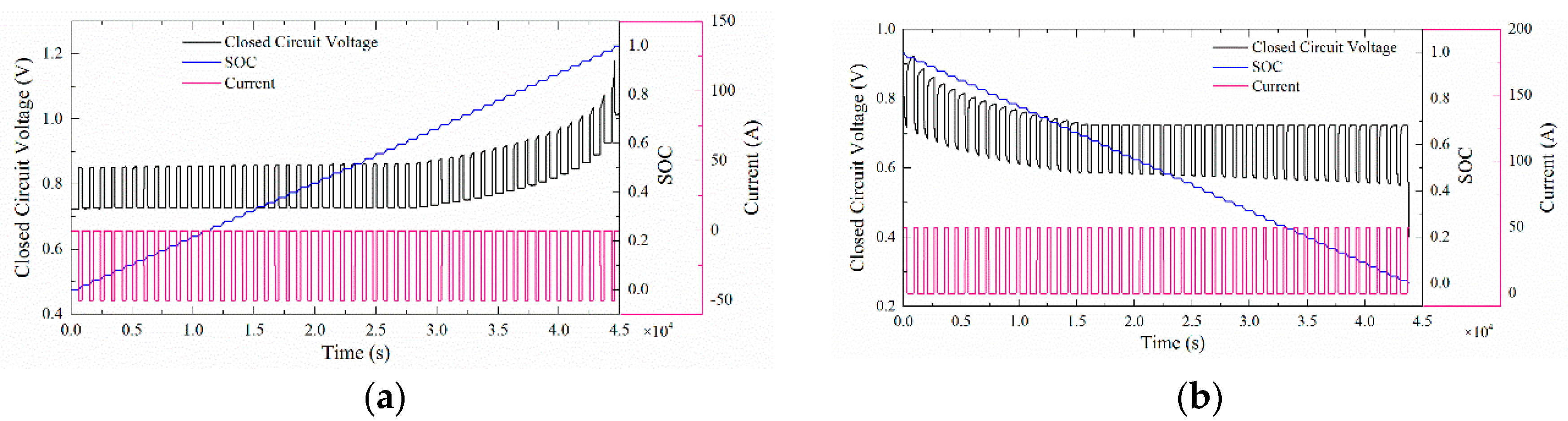
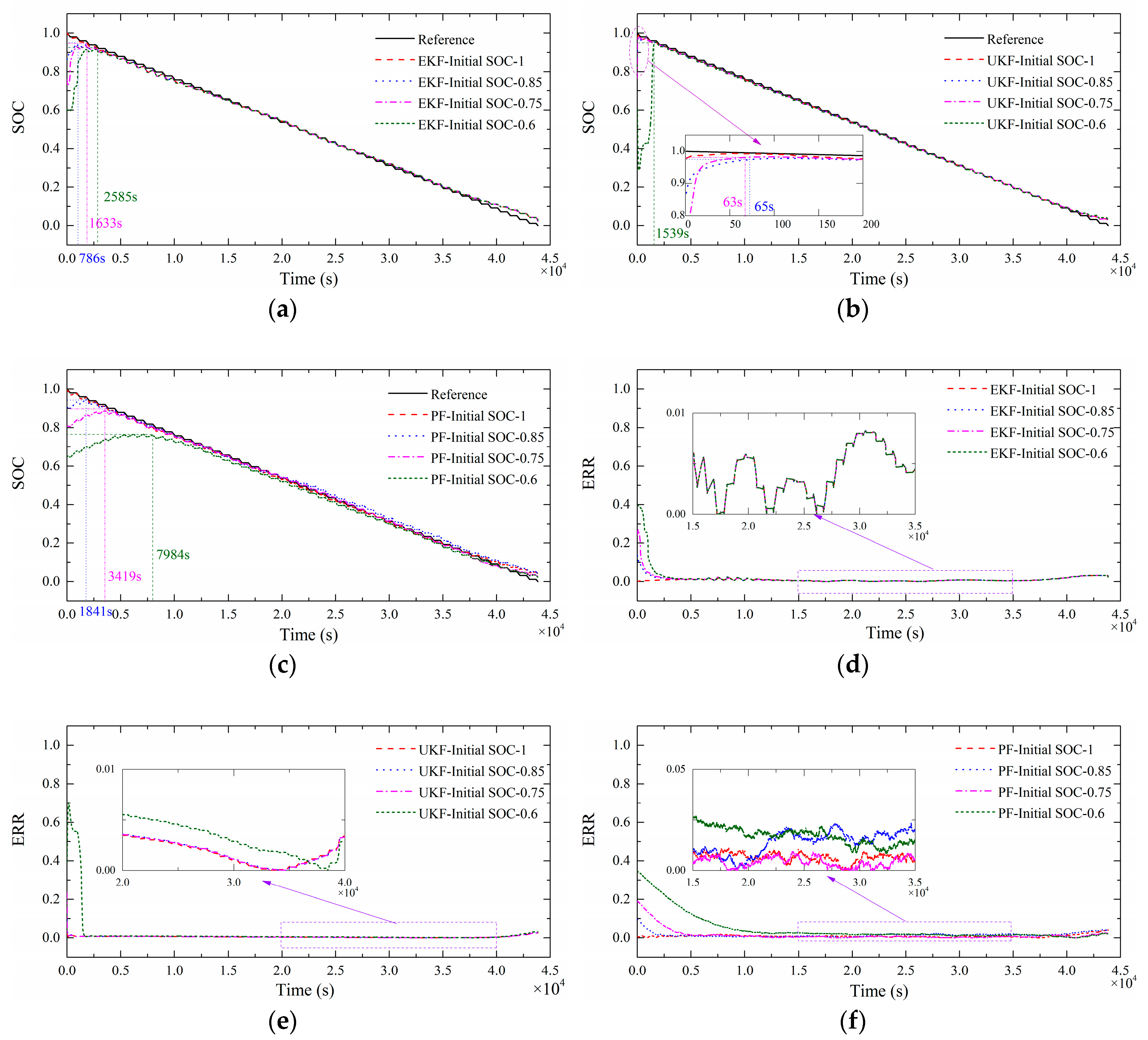
5.1. SoC Estimation Results in Pulse Discharge Mode

The properties of Li-Bi LMBs, particularly the quasi-static SoC-OCV relationship when the SoC is between 65% and 0%, can be used to explain the results of estimation. We note from Figure 6 that when the UKF algorithm is applied for estimation in the pulse discharge scenario, the results converge to the actual SoC after 63 and 65 s, respectively, with initial settings of 0.85 and 0.75. In contrast, convergence only occurs after 1539 s when the initial SoC is 0.6. When the EKF and PF algorithms are used for estimation, the convergence time with an initial SoC of 0.6 is about twice of that obtained with an initial SoC of 0.75.

We observe that, with the PF algorithm, the convergence time increases in proportion to the magnitude of deviation between the initial value and the true SoC value. The partially enlarged plots in the insets to subfigures (d–f) indicate that after convergence, the estimation error distributions obtained using the EKF algorithm were consistent, regardless of the initial SoC. In contrast, while the distributions obtained using the UKF algorithm were consistent when the initial SoCs were above 0.65, these values differed from the one obtained with an initial SoC below 0.65. We also note that the error distributions change irregularly throughout the estimation. To highlight the differences in performance observed with the different algorithms and initial values, the RMSE of the SoC estimates for the complete test period and the value obtained after convergence, are listed in Table 5, together with the convergence times. Our results indicate that the estimates obtained using the EKF and UKF algorithms, with different initial SoCs, are convergent. The estimation of the SoC with SoC₀ set as 1 is used to evaluate the accuracy of the three algorithms. The RMSE of EKF algorithm and UKF algorithm are 0.0118 and 0.0063, respectively, indicating that for the SoC estimation, the UKF algorithm has a higher accuracy. The difference between the two algorithms is mainly caused by the modelling error.

In the PF algorithm, particles described by a Gaussian distribution are used to describe the state estimation distribution probability and resampling is applied. So, the estimation results may not change smoothly like the other two algorithms. The RMSE after convergence using PF algorithm with different SoC₀ are 0.0114, 0.0158, 0.0092 and 0.0188, varying substantially, indicating that this algorithm may not be suitable for the SoC estimation of LMB. Since, this is a device that is hard to determine the initial SoC accurately.

The difference between overall RMSE and RMSE after convergence is caused mainly of the difference between the SoC₀ set at the beginning of the estimation and the difference between them can be reduced by expanding the experimental time. The greater difference between the SoC₀ and the actual SoC value is, the greater difference between overall RMSE and RMSE after convergence will be. The overall RMSE and RMSE after convergence shows little difference in UKF algorithm with SoC₀ set as 0.85 and 0.75 proving the ability of this algorithm in eliminating the influence of the initial value.

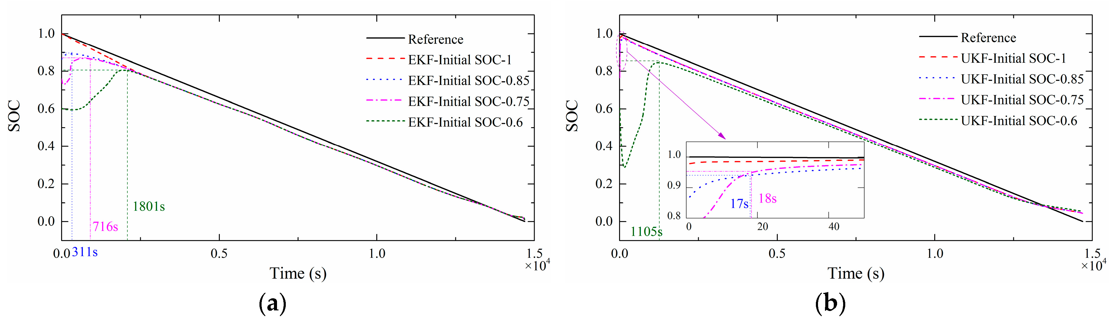
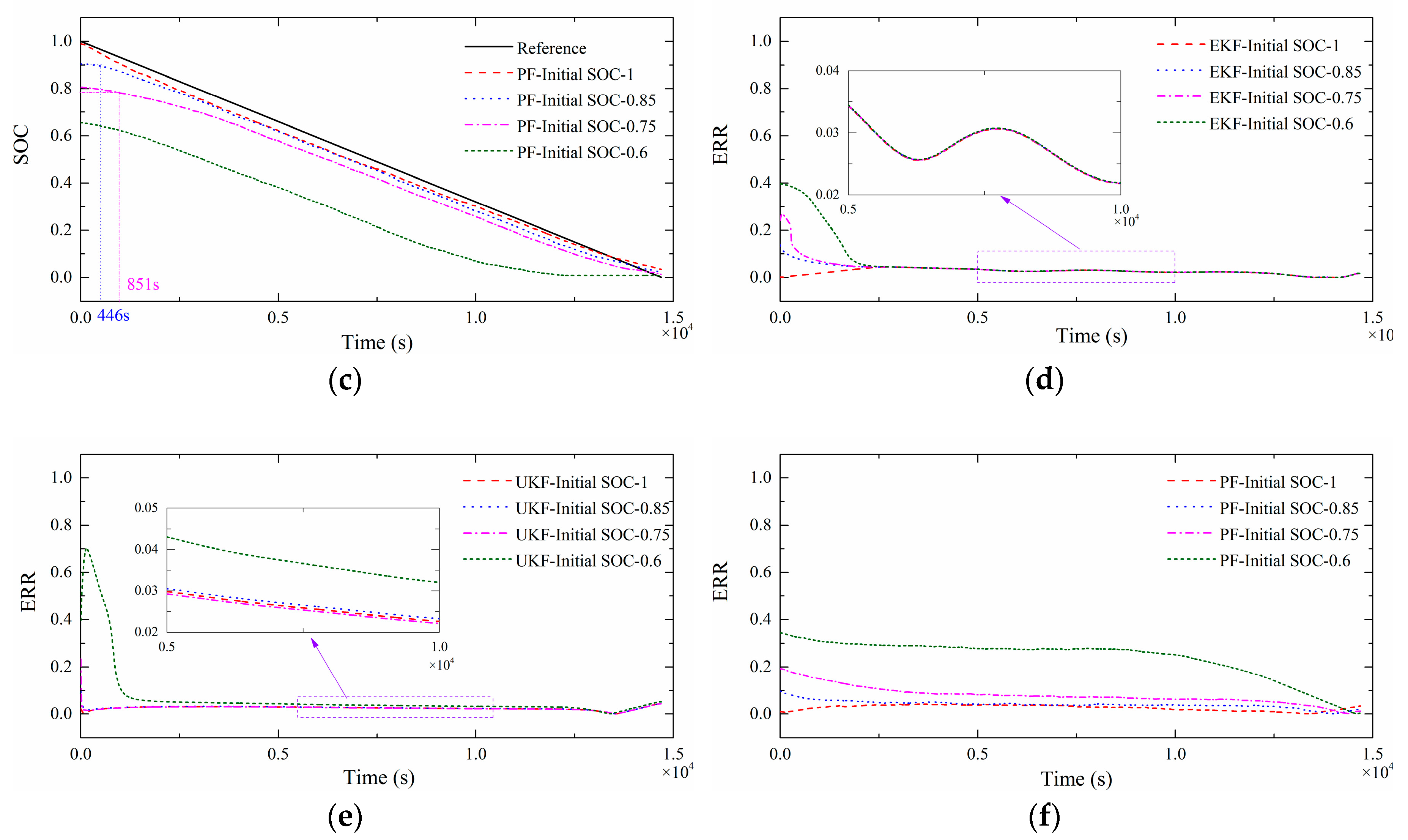
5.2. SoC Estimation Results in Current Discharge Mode

We note a similar convergence characteristic for the different algorithms in Figure 7. However, the PF algorithm failed in scenario (b). The failure of the PF algorithm is due to the poor distribution of particles and the invariant working current. The RMSEs of the SoC estimates after convergence are listed in Table 6, together with the convergence times. Scenarios (a) and (b) both simulate battery operation in a relatively stable state, explaining the similarities in the performance of the algorithms.

The error between the estimated and reference SoC in scenario (b) is higher than that observed in scenario (a). This is because the SoC of a battery is reduced as it discharges. As previously noted, the OCV is insensitive to SoC when this value is below 65%. However, since a polarization voltage is generated when the current changes (when pulses are applied), the insensitivity of OCV to SoCs below 65% can be compensated, reducing the error in the estimate obtained in scenario (a). In contrast, the current is static in the constant current profile of scenario (b). As a result, SoC estimation depends on Coulombic accumulation, which intensifies errors. We observed a significant increase in error at 13500 s, with all three algorithms investigated, when the SoC was close to zero. This can be explained by the fact that there is a rapid decline in voltage at the end of the discharge process, while the OCV remains unchanged. With little compensation from polarization voltage, the reduced sensitivity of OCV and R_o to SoC cause a calculation error.

The overall RMSE and RMSE after convergence using all three algorithms in scenario (b) are larger than that in scenario (a) show that these algorithms have difficulty in dealing with a long-lasting constant working condition. The UKF algorithm works better than the others.

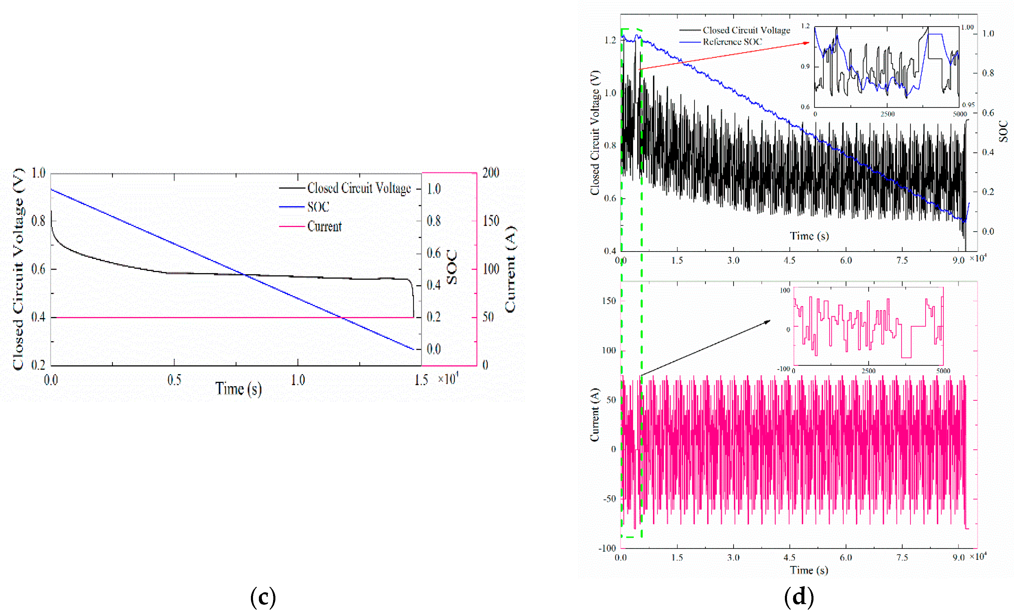
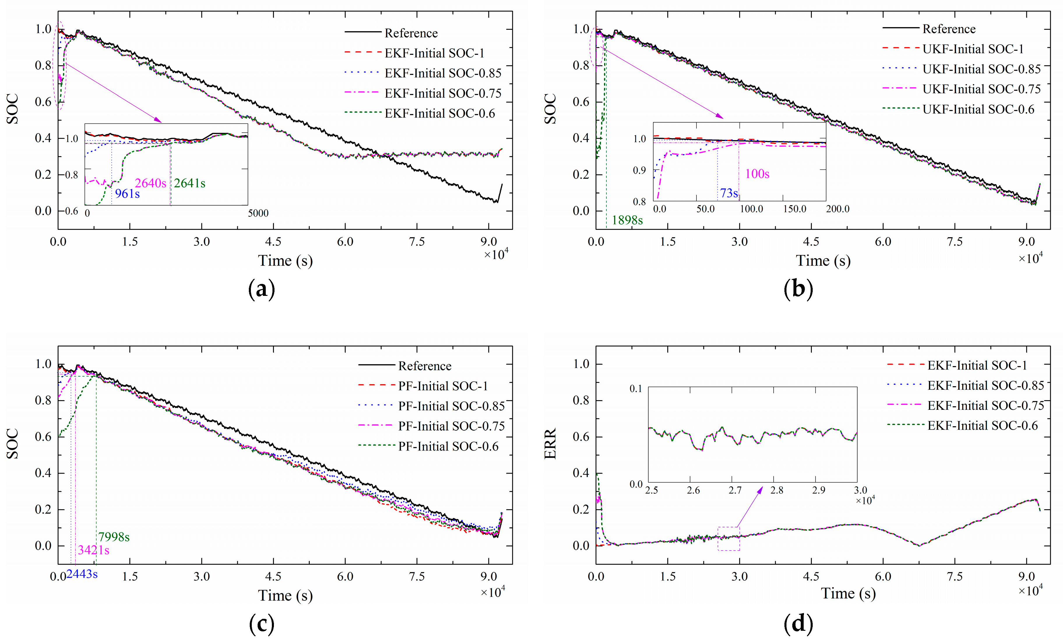
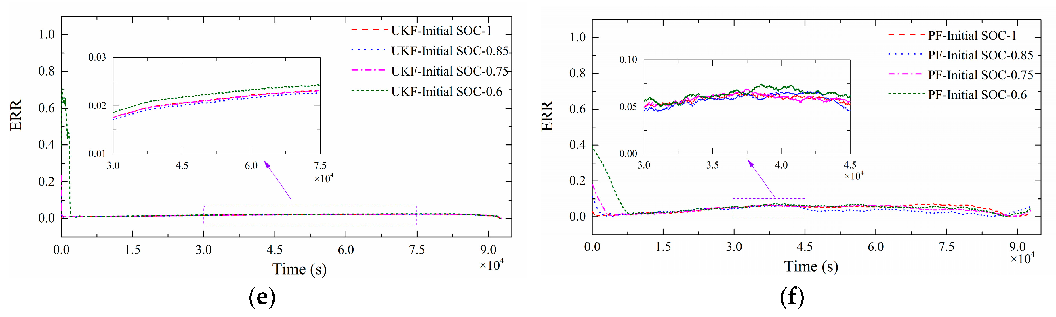
5.3. SoC Estimation Results in Hybrid Pulse Charge/Discharge

From Figure 8, we are able to observe clear distinctions in the behavior of the three algorithms. Although they all converge to the reference value initially, with the EKF algorithm, the estimation error began to grow after 4 h, eventually reaching a maximum of 0.3. While the estimates obtained with the PF algorithm mirrored the changes to the actual SoC, there were large errors between the different values. We note a similar convergence characteristic with the PF algorithm in Figure 6 and Figure 8. In contrast, with the UKF algorithm, after convergence, the estimates reflected the changes to the actual SoC, with an RMSE of about 0.019, even when the SoC was below 65%. In addition, convergence was quicker with this algorithm than it was with the PF and EKF, indicating it had the best overall performance of the techniques considered. The RMSEs of the SoC estimates after convergence are listed in Table 7, together with the convergence times. From this, we note that with the EKF and UKF algorithms, the RMSEs are larger and the distribution is more consistent, regardless of the initial SoC, than the results obtained in application scenario (a) and (b).

The estimation errors observed with these results can partly be explained by the conditions defined for scenario (c). The fluctuations in the current profiles have an effect on SoC estimation, as discussed earlier in the comparison between Figure 6 and Figure 7. The experiment was conducted for 25 h, after which the total capacity of the battery, which has a self-discharge current of 0.4 A, had been reduced to nearly 5%. As this self-discharge current is negligible compared to the working current of the cell, it is ignored in the ECN model and the capacity of the battery remains constant at 200 Ah. Hence, real-time update of the battery capacity, according to parameters such as the working current, working time and cycle life may improve the accuracy of the algorithms.

5.4. Further Discussion

We note from a comparison of Figure 6, Figure 7 and Figure 8, that the UKF algorithm shows the most stable convergence characteristic, while the EKF algorithm fails in long-lasting estimation and the PF algorithm fails with the constant current profile. Convergence was quickest with the UKF algorithm and there was little change in the RMSE of the overall SoC estimates and the values obtained after convergence, which were about 0.007, 0.026 and 0.019 in scenarios (a), (b) and (c), respectively. Convergence was longer with the EKF algorithm, after which the RMSE of the SoC estimates remained relatively stable at about 0.012, 0.03 and 0.10 for scenarios (a), (b) and (c), respectively. The PF algorithm required the longest time for convergence. In addition, SoC estimation was much more accurate in scenarios (a) and (c), than in scenario (b).

We also note that the convergence time increases when the SoC₀ set in the calculation is decreased. This can be explained by the characteristic of the LMB. When the SoC₀ is set as 0.6, it is below 0.65. This device has a quasi-static OCV-SoC relationship when the SoC changes between 0 to 0.65 while the R_o-SoC curve is not obvious either. So, the observational values calculated by the state estimates in the algorithms changes little at the beginning of the simulation and more steps are needed to converge the difference between estimated and actual observational values, which means more convergence time. When the SoC₀ are set above 0.65, such as 0.85 and 0.75, both the OCV-SoC curve and the R_o-SoC curve are more obvious, the convergence is much easier to be achieved. As the LMB is fully charged at the beginning of the experiments in all three scenarios, SoC₀ set as 0.85 is closer to the real initial value than SoC₀ set as 0.75, resulting in a shorter convergence time than the latter one.

The computation times of the three algorithms in the different scenarios, as well as the duration of testing, are also considered and shown in

Table 8. Computation time for SoC estimation.

Algorithm	Scenario (a)	Scenario (b)	Scenario (c)
EKF	11.908 (s)	4.13 (s)	25.863 (s)
UKF	23.717 (s)	8.291 (s)	52.215 (s)
PF	73.820 (s)	24.810 (s)	158.264 (s)
Test time	12.179 (h)	4.081 (h)	25.778 (h)

. Computation is quickest with the EKF algorithm, which spends approximately 0.26 ms making one estimation. As the evaluation of Jacobi matrices ((6) and (7)) accounts for half of the computation time, it can be said that the complexity of calculation is primarily influenced by the battery model. The UKF algorithm spends almost twice as much time in computation than the EKF algorithm, meaning that it takes about 0.5 ms to make one estimation. Calculation of the four iterative functions (4)–(7) takes about 61.9% of the total simulation time, indicating that the speed of computation could be improved if the battery model could be simplified and the order of the functions could be reduced without compromising their accuracy. Finally, while computation with the PF algorithm is about three times longer than it is with the UKF, taking about 1.5 ms to make one estimation, this increased duration does not lead to an improved SoC estimate.

To verify that increased algorithmic complexity could improve the accuracy of estimation, we also tested the performance of the PF algorithm with 100 particles (PF (100)), instead of 20 particles (PF (20)). The RMSEs and the time spent in estimation are listed in

Table 9. RMSE and calculation time for SoC estimation in scenarios (a)–(c) using PF (100) and PF (20) with different SoC₀ values.

Algorithm	SoC0	Scenario (a)	Scenario (b)	Scenario (c)
PF (100)	1	0.0296	0.0274	0.0412
	0.85	0.0184	0.0323	0.0505
	0.75	0.0357	0.0563	0.0507
	0.6	0.0672	0.2051	0.0761
	Time	397.378 (s)	132.327 (s)	918.940 (s)
PF (20)	1	0.0114	0.0288	0.0486
	0.85	0.0195	0.0429	0.0373
	0.75	0.0327	0.0871	0.0486
	0.6	0.0857	0.2524	0.0818
	Time	73.820 (s)	24.810 (s)	158.264 (s)

, where we are able to note that although the computation time increased by a factor of six with these experiments, any reductions in the RMSE were negligible, indicating that the PF algorithm may not be suitable for Li-Bi LMBs.

6. Conclusions

In this paper, we have introduced the properties of Li-Bi LMBs, to illustrate the difficulties involved in using traditional SoC estimation techniques. We note that open-circuit-voltage and Coulombic counting methods are unsuitable for these devices, because of a partially quasi-static OCV-SoC relationship and the difficulties involved in determining the initial SoC. Hence, we established an ECN battery model and explored the performance of the extended Kalman filter, the unscented Kalman filter and the particle filter for SoC estimation, using three current profiles: a constant current discharge profile, a pulse discharge profile and a hybrid pulse profile comprising charging and discharging processes. The first two scenarios consider ideal working conditions, while the last one simulates a more realistic mode of operation. In a reflection of the properties of LMBs, the RMSE is very small when the initial SoC is above 0.65 and rises when this is below 0.65. Since SoC estimation is difficult with a constant working current, the variation that occurs above 0.65 enables accurate completion of this estimation process, to overcome the difficulties caused by the quasi-static region of OCV-SoC curve. Our results indicate that the UKF algorithm gives the best overall performance for all the current profiles considered. In particular, in dynamic working conditions, we obtained RMSEs below 0.02, with this algorithm. Although EKF performs well in relatively stable conditions and can complete operations at twice the speed of the UKF, the magnitude of the estimation errors increases with the duration of monitoring. While the PF algorithm works well when the initial SoC is close to the actual value, it is better optimized for operation in dynamic rather than static conditions, where it risks failure. The computation time of this algorithm is also about six times longer than that of the EKF or three times longer than the UKF. As the intended application of the battery is as part of a power grid, where its mode of operation will change frequently without schedule, monitoring is necessarily real-time and long-lasting. Based on these characteristics, the UKF algorithm is most suitable for battery management system because it converges quickly to an accurate SoC estimate.

To improve SoC estimation performance, future work will concentrate on developing a simpler, more accurate battery model and the possible adoption of on-line parameter identification. As a battery model considering self-discharge is recommended for long-time SoC estimation, the inclusion of relationships between battery parameters and SoC at different working currents will increase the accuracy of the battery model. Further experiments determining other parameters sensitive to current, for creation of a different model and studying the capacity attenuation mechanism, will be conducted. Finally, as we only considered a constant operating temperature in this study, future work will also concentrate on SoC estimation in more varied temperature environments.

References

1. Soloveichik, G.L. Battery technologies for large-scale stationary energy storage. Annu. Rev. Chem. Biomol. Eng. 2011, 2, 503–527. [Google Scholar] [CrossRef] [PubMed]
2. Wang, K.; Jiang, K.; Chung, B.; Ouchi, T.; Burke, P.J.; Boysen, D.A.; Bradwell, D.J.; Kim, H.; Muecke, U.; Sadoway, D.R. Lithium-antimony-lead liquid metal battery for grid-level energy storage. Nature 2014, 514, 348–350. [Google Scholar] [CrossRef] [PubMed]
3. Ashour, R.F.; Kelley, D.H.; Salas, A.; Starace, M.; Weber, N.; Weier, T. Competing forces in liquid metal electrodes and batteries. J. Power Sources 2018, 378, 301–310. [Google Scholar] [CrossRef] [Green Version]
4. Bradwell, D.J.; Kim, H.; Sirk, A.H.; Sadoway, D.R. Magnesium-antimony liquid metal battery for stationary energy storage. J. Am. Chem. Soc. 2012, 134, 1895–1897. [Google Scholar] [CrossRef] [PubMed]
5. Kim, H.; Boysen, D.A.; Newhouse, J.M.; Spatocco, B.L.; Chung, B.; Burke, P.J.; Bradwell, D.J.; Jiang, K.; Tomaszowska, A.A.; Wang, K.; et al. Liquid metal batteries: Past, present, and future. Chem. Rev. 2013, 113, 2075–2099. [Google Scholar] [CrossRef] [PubMed]
6. Newhouse, J.M. Modeling the Operating Voltage of Liquid Metal Battery Cells. Ph.D. Thesis, MIT, Cambridge, MA, USA, 2014. [Google Scholar]
7. Ning, X.; Phadke, S.; Chung, B.; Yin, H.; Burke, P.; Sadoway, D.R. Self-healing Li–Bi liquid metal battery for grid-scale energy storage. J. Power Sources 2015, 275, 370–376. [Google Scholar] [CrossRef] [Green Version]
8. Wei, Z.; Leng, F.; He, Z.; Zhang, W.; Li, K. Online state of charge and state of health estimation for a Lithium-Ion battery based on a data–model fusion method. Energies 2018, 11, 1810. [Google Scholar] [CrossRef]
9. Liu, S.; Cui, N.; Zhang, C. An Adaptive Square Root Unscented Kalman Filter Approach for State of Charge Estimation of Lithium-Ion Batteries. Energies 2017, 10, 1345. [Google Scholar] [Green Version]
10. Piller, S.; Perrin, M.; Jossen, A. Methods for state-of-charge determination and their applications. J. Power Sources 2001, 96, 113–120. [Google Scholar] [CrossRef]
11. He, H.; Zhang, X.; Xiong, R.; Xu, Y.; Guo, H. Online model-based estimation of state-of-charge and open-circuit voltage of lithium-ion batteries in electric vehicles. Energy 2012, 39, 310–318. [Google Scholar] [CrossRef]
12. Chiang, Y.H.; Sean, W.Y.; Ke, J.C. Online estimation of internal resistance and open-circuit voltage of lithium-ion batteries in electric vehicles. J. Power Sources 2011, 196, 3921–3932. [Google Scholar] [CrossRef]
13. Lee, S.; Kim, J.; Lee, J.; Cho, B. State-of-charge and capacity estimation of lithium-ion battery using a new open-circuit voltage versus state-of-charge. J. Power Sources 2008, 185, 1367–1373. [Google Scholar] [CrossRef]
14. Hu, X.S.; Sun, F.C.; Zou, Y.A. Estimation of state of charge of a lithium-ion battery pack for electric vehicles using an adaptive luenberger observer. Energies 2010, 3, 1586–1603. [Google Scholar] [CrossRef]
15. Chin, C.; Gao, Z. State-of-charge estimation of battery pack under varying ambient temperature using an adaptive sequential extreme learning machine. Energies 2018, 11, 711. [Google Scholar] [CrossRef]
16. Piao, C.H.; Fu, W.L.; Lei, G.H.; Cho, C.D. Online parameter estimation of the Ni-MH batteries based on statistical methods. Energies 2010, 3, 206–215. [Google Scholar] [CrossRef]
17. Hansen, T.; Wang, C.J. Support vector based battery state of charge estimator. J. Power Sources 2005, 141, 351–358. [Google Scholar] [CrossRef]
18. Anton, J.A.; Nieto, P.G.; Viejo, C.B.; Vilan, J.V. Support vector machines used to estimate the battery state of charge. IEEE Trans. Power Electron. 2013, 28, 5919–5926. [Google Scholar] [CrossRef]
19. Hu, J.N.; Hu, J.J.; Lin, H.B.; Li, X.P.; Jiang, C.L.; Qiu, X.H.; Li, W.S. State-of-charge estimation for battery management system using optimized support vector machine for regression. J. Power Sources 2014, 269, 682–693. [Google Scholar] [CrossRef]
20. Chen, L.; Wang, Z.; Lü, Z.; Li, J.; Ji, B.; Wei, H.; Pan, H. A novel state-of-charge estimation method of lithium-ion batteries combining the Grey model and Genetic Algorithms. IEEE Trans. Power Electron. 2018, 33, 8797–8807. [Google Scholar] [CrossRef]
21. Singh, P.; Vinjamuri, R.; Wang, X.; Reisner, D. Design and implementation of a fuzzy logic-based state-of-charge meter for Li-ion batteries used in portable defibrillators. J. Power Sources 2006, 162, 829–836. [Google Scholar] [CrossRef]
22. Waag, W.; Fleischer, C.; Sauer, D.U. Critical review of the methods for monitoring of lithium-ion batteries in electric and hybrid vehicles. J. Power Sources 2014, 258, 321–339. [Google Scholar] [CrossRef]
23. Plett, G.L. Extended Kalman filtering for battery management systems of LiPB-based HEV battery packs: Part 1. Background. J. Power Sources 2004, 134, 252–261. [Google Scholar] [CrossRef]
24. Lee, K.T.; Dai, M.J.; Chuang, C.C. Temperature-compensated model for lithium-ion polymer batteries with extended Kalman filter state-of-charge estimation for an implantable charger. IEEE Trans. Ind. Electron. 2018, 65, 589–596. [Google Scholar] [CrossRef]
25. He, H.; Xiong, R.; Zhang, X.; Sun, F.; Fan, J.X. State-of-charge estimation of the lithium-ion battery using an adaptive extended Kalman filter based on an improved Thevenin model. IEEE Trans. Veh. Technol. 2011, 60, 1461–1469. [Google Scholar]
26. Yang, J.; Xia, B.; Shang, Y.; Huang, W.; Mi, C.C. Adaptive state-of-charge estimation based on a split battery model for electric vehicle applications. IEEE Trans. Veh. Technol. 2017, 66, 10889–10898. [Google Scholar] [CrossRef]
27. Plett, G.L. Sigma-point Kalman filtering for battery management systems of LiPB-based HEV battery packs: Part 1: Introduction and state estimation. J. Power Sources 2006, 161, 1356–1368. [Google Scholar] [CrossRef]
28. Liu, C.; Liu, W.; Wang, L.; Hu, G.; Ma, L.; Ren, B. A new method of modeling and state of charge estimation of the battery. J. Power Sources 2016, 320, 1–12. [Google Scholar] [CrossRef]
29. Schwunk, S.; Armbruster, N.; Straub, S.; Kehl, J.; Vetter, M. Particle filter for state of charge and state of health estimation for lithium–iron phosphate batteries. J. Power Sources 2013, 239, 705–710. [Google Scholar] [CrossRef]
30. Dong, G.; Chen, Z.; Wei, J.; Zhang, C.; Wang, P. An online model-based method for state of energy estimation of lithium-ion batteries using dual filters. J. Power Sources 2016, 301, 277–286. [Google Scholar] [CrossRef]
31. Hua, Y.; Cordoba-Arenas, A.; Warner, N.; Rizzoni, G. A multi time-scale state-of charge and state-of-health estimation framework using nonlinear predictive filter for lithium-ion battery pack with passive balance control. J. Power Sources 2015, 280, 293–312. [Google Scholar] [CrossRef]
32. Hu, C.; Youn, B.D.; Chung, J. A multiscale framework with extended Kalman filter for lithium-ion battery SOC and capacity estimation. Appl. Energy 2012, 92, 694–704. [Google Scholar] [CrossRef]
33. Pan, H.; Lü, Z.; Lin, W.; Li, J.; Chen, L. State of charge estimation of lithium-ion batteries using a grey extended kalman filter and a novel open-circuit voltage model. Energy 2017, 138, 764–775. [Google Scholar] [CrossRef]
34. Wei, J.; Dong, G.; Chen, Z. On-board adaptive model for state of charge estimation of lithium-ion batteries based on Kalman filter with proportional integral-based error adjustment. J. Power Sources 2017, 365, 308–319. [Google Scholar] [CrossRef]
35. Lim, K.; Bastawrous, H.A.; Duong, V.H.; See, K.W.; Zhang, P.; Dou, S.X. Fading Kalman filter-based real-time state of charge estimation in LiFePO4 battery-powered electric vehicles. Appl. Energy 2016, 169, 40–48. [Google Scholar] [CrossRef]
36. Liu, X.; Chen, Z.; Zhang, C.; Wu, J. A novel temperature-compensated model for power Li-ion batteries with dual-particle-filter state of charge estimation. Appl. Energy 2014, 123, 263–272. [Google Scholar] [CrossRef]
37. Cai, M.; Chen, W.; Tan, X. Battery state-of-charge estimation based on a dual unscented Kalman filter and fractional variable-order model. Energies 2017, 10, 1577. [Google Scholar] [CrossRef]
38. Xiong, R.; Sun, F.; Chen, Z.; He, H. A data-driven multi-scale extended Kalman filtering based parameter and state estimation approach of lithium-ion polymer battery in electric vehicles. Appl. Energy 2014, 113, 463–476. [Google Scholar]
39. Tran, N.T.; Khan, A.B.; Choi, W. State of Charge and State of Health Estimation of AGM VRLA Batteries by Employing a Dual Extended Kalman Filter and an ARX Model for Online Parameter Estimation. Energies 2017, 10, 137. [Google Scholar] [CrossRef]
40. Li, Y.; Chattopadhyay, P.; Xiong, S.; Ray, A.; Rahn, C.D. Dynamic data-driven and model-based recursive analysis for estimation of battery state-of-charge. Appl. Energy 2016, 184, 266–275. [Google Scholar] [CrossRef]
41. Propp, K.; Auger, D.J.; Fotouhi, A.; Longo, S.; Knap, V. Kalman-variant estimators for state of charge in lithium-sulfur batteries. J. Power Sources 2017, 343, 254–267. [Google Scholar] [CrossRef] [Green Version]
42. Fotouhi, A.; Auger, D.J.; Propp, K.; Longo, S. Lithium-sulfur battery state-of-charge observability analysis and estimation. IEEE Trans. Power Electron. 2018, 33, 5847–5859. [Google Scholar] [CrossRef]
43. Pickard, W.F.; Shen, A.Q.; Hansing, N.J. Parking the power: Strategies and physical limitations for bulk energy storage in supply–demand matching on a grid whose input power is provided by intermittent sources. Renew. Sustain. Energy Rev. 2009, 13, 1934–1945. [Google Scholar] [CrossRef]
44. Kroeze, R.C.; Krein, P.T. Electrical battery model for use in dynamic electric vehicle simulations. In Proceedings of the 2008 IEEE Power Electronics Specialists Conference, Rhodes, Greece, 15–19 June 2008; pp. 1336–1342. [Google Scholar]
45. Gao, W.; Jiang, M.; Hou, Y. Research on PNGV model parameter identification of LiFePO4 Li-ion battery based on FMRLS. In Proceedings of the 2011 6th IEEE Conference on Industrial Electronics and Applications, Beijing, China, 21–23 June 2011; pp. 2294–2297. [Google Scholar]
46. Yao, L.W.; Wirun, A.; Aziz, M.J.B.A.; Sutikno, T. Battery state-of-charge estimation with extended Kalman-filter using third-order Thevenin model. Telkomnika 2015, 13, 401–412. [Google Scholar] [CrossRef]
47. Freedom CAR Program Electrochemical Energy Storage Team. Freedom CAR Battery Test Manual for Power Assist Hybrid Electric Vehicles; U.S. Department of Energy: Washington, DC, USA, 2003.
48. Hoque, M.M.; Hannan, M.A.; Mohamed, A. Charging and discharging model of lithium-ion battery for charge equalization control using particle swarm optimization algorithm. J. Renew. Sustain. Energy 2016, 8, 7847–7858. [Google Scholar] [CrossRef]
49. Rahman, M.A.; Anwar, S.; Izadian, A. Electrochemical model parameter identification of a lithium-ion battery using particle swarm optimization method. J. Power Sources 2016, 307, 86–97. [Google Scholar] [CrossRef]
50. Guo, X.; Kang, L.; Yao, Y.; Huang, Z.; Li, W. Joint estimation of the electric vehicle power battery state of charge based on the least squares method and the Kalman filter algorithm. Energies 2016, 9, 100. [Google Scholar] [CrossRef]
51. Zhan, R.; Wan, J. Neural network-aided adaptive unscented Kalman filter for nonlinear state estimation. IEEE Signal Process. Lett. 2006, 13, 445–448. [Google Scholar] [CrossRef]
52. An, D.; Choi, J.H.; Kim, N.H. Prognostics 101: A tutorial for particle filter-based prognostics algorithm using Matlab. Reliab. Eng. Syst. Saf. 2013, 115, 161–169. [Google Scholar] [CrossRef]
53. Li, T.; Bolic, M.; Djuric, P.M. Resampling Methods for Particle Filtering: Classification, implementation, and strategies. IEEE Signal Process. Mag. 2015, 32, 70–86. [Google Scholar] [CrossRef]
54. Jouin, M.; Gouriveau, R.; Hissel, D.; Péra, M.C.; Zerhouni, N. Particle filter-based prognostics: Review, discussion and perspectives. Mech. Syst. Signal Process. 2016, 72–73, 2–31. [Google Scholar] [CrossRef]
Figure 1. Schematic of charge and discharge processes in a liquid metal battery (LMB).
Energies 12 00183 g001
Figure 2. Experimental setup.
Energies 12 00183 g002
Figure 3. Terminal voltage, reference SoC and current profiles obtained in: (a) pulse charge; (b) pulse discharge; (c) constant current discharge and (d) hybrid pulse current charge and discharge modes of operation.
Energies 12 00183 g003aEnergies 12 00183 g003b
Figure 4. Equivalent circuit model of a Li-Bi LMB.
Energies 12 00183 g004
Figure 5. Parameter identification curves for OCV, Ro, C1 and R1 with respect to SoC: (a) OCV-SoC; (b) Ro-SoC; (c) C1-SoC; (d) R1-SoC.
Energies 12 00183 g005
Figure 6. Comparison of SoC measured in pulse discharge mode (scenario (a)) with estimates made using different initial values (SoC0): (a) SoC estimation using EKF; (b) SoC estimation using UKF; (c) SoC estimation using PF; (d) Error of SoC estimation using EKF; (e)Error of SoC estimation using UKF; (f) Error of SoC estimation using PF.
Energies 12 00183 g006
Figure 7. Comparison of SoC measured in constant current discharge mode (scenario (b)) with estimates made using different values of SoC0: (a) SoC estimation using EKF; (b) SoC estimation using UKF; (c) SoC estimation using PF; (d) Error of SoC estimation using EKF; (e) Error of SoC estimation using UKF; (f) Error of SoC estimation using PF.
Energies 12 00183 g007aEnergies 12 00183 g007b
Figure 8. Comparison of SoC measured in hybrid pulse charge/discharge mode (scenario (c)) with estimates made using different values of SoC0: (a) SoC estimation using EKF; (b) SoC estimation using UKF; (c) SoC estimation using PF; (d) Error of SoC estimation using EKF; (e) Error of SoC estimation using UKF; (f) Error of SoC estimation using PF.
Energies 12 00183 g008aEnergies 12 00183 g008b