Article

An Aero-acoustic Noise Distribution Prediction Methodology for Offshore Wind Farms

1
School of Hydraulic Energy and Power Engineering, Yangzhou University, Yangzhou 225127, China
2
Jiangsu Key Laboratory of Hi-Tech Research for Wind Turbine Design, Nanjing University of Aeronautics and Astronautics, Nanjing 211100, China
3
GCL Intelligent Energy Co., Ltd., Suzhou 215000, China
*
Author to whom correspondence should be addressed.
Energies 2019, 12(1), 18; https://doi.org/10.3390/en12010018
Submission received: 28 November 2018 / Revised: 17 December 2018 / Accepted: 19 December 2018 / Published: 21 December 2018
(This article belongs to the Special Issue Recent Advances in Offshore Wind Technology)

Abstract

:
Recently attention has been paid to wind farm noise due to its negative health impact, not only on human beings, but also to marine and terrestrial organisms. The current work proposes a numerical methodology to generate a numerical noise map for a given wind farm. Noise generation from single wind turbines as well as wind farms has its basis in the nature of aerodynamics, caused by the interactions between the incoming turbulent flow and the wind turbine blades. Hence, understanding the mechanisms of airfoil noise generation, demands access to sophisticated numerical tools. The processes of modeling wind farm noise include three steps: (1) The whole wind farm velocity distributions are modelled with an improved Jensen’s wake model; (2) The individual wind turbine’s noise is simulated by a semi-empirical wind turbine noise source model; (3) Propagations of noise from all wind turbines are carried out by solving the parabolic wave equation. In the paper, the wind farm wake effect from the Horns Rev wind farm is studied. Based on the resulted wind speed distributions in the wind farm, the wind turbine noise source and its propagation are simulated for the whole wind farm.

1. Introduction

With the fast increase of blade length as well as the number of wind farms, more environmental impact is expected to occur such as excessive wind turbine noise emissions. Extraction of more energy from wind is obviously the key design target of wind farm developers. However, total energy yield and aerodynamic noise generation are usually two competing variables. Due to the more pronounced wind farm noise issue, there is clearly a need to develop sophisticated design tools to fulfil the requirements of wind farm’s high power performance and low noise radiation. Previous works were more focused on individual wind turbine noise source predictions. Therefore, for a long time wind turbine noise studies have been separated from wind turbine noise source generation and noise propagation. As wind farm noise has now become an essential research topic, the objective of the current work is to couple a wind farm wake model with a wind farm noise source model and finally generate the wind farm noise map using a long range noise propagation method. Above the sea, noise generated from offshore wind farms may travel kilometers to reach the nearby dwellers, but there are two facts which enhance offshore wind farm noise propagation: (1) no noise barrier exists over the propagation range; (2) the water surface is acoustically hard and almost fully reflective. Noise propagation under sea is more related to marine organisms. The cumulative effect of noise from offshore wind farms is a challenging task which requires years of study. Previous work done by Andersson [1] found out that species could detect a wind farm at a distance of several kilometres up to tens of kilometres. Owing to the restricted knowledge of hearing sense, the current work will only focus on numerical prediction of noise propagation in a wind farm. From the numerical aspect, modeling of large wind farm noise is a cross disciplinary task which requires knowledge of aeroacoustics, wind turbine aerodynamics and atmospheric acoustics. For such a purpose, a new computational framework is built to couple flow with acoustic propagation in large offshore wind farms.
For wind turbines inside a wind farm, it is known that the velocity deficit causes momentum loss in the wake and therefore decreases the energy product of the downstream wind turbines. Accurate modeling of wake deficit is of significant importance, not only for energy estimation but also for wind turbine noise source prediction. The velocity at each rotor plan is the key parameter to model wind turbine aerodynamic noise. High wind velocity correlates to high power output, but usually generates higher aerodynamics noise, this is often a contradiction for designing high power and low noise wind farms. A review of various wake models was presented by Göçmen et al. [2] where six widely used wake modeling approaches were discussed. Based on the studies of some operating wind farms, there is evidently a continuous need to find accurate and robust wind farm wake models. Computational Fluid Dynamics (CFD)-based Actuator Disc (AD) [3,4,5] and Actuator Line (AL) methods [6,7,8] represent the future trend for detailed wind farm analysis, but due to the heavy computational effort, the current wind farm layout design tools are highly reliant on engineering methods. In the short term, the conventional models based on Jensen, Frandsen and Larsen’s approaches [9,10,11,12] are the major tools. Based on the previous development, a new two dimensional Jensen’s model [13,14] is applied in the current work which maintains the same efficiency but with improved accuracy.
The wake deficit at each rotor disc not only influences the energy production but also the aerodynamic noise level. When the incoming wind speed is captured by the wake model, the aerodynamic noise can be calculated. Full Computational Aero-Acoustic (CAA) computation for a wind farm is far from reality, CAA is even rarely applied for a single wind turbine with today’s High Performance Computers (HPCs). Like wind farm wake analyses, an alternative approach is to apply well validated engineering methods. An airfoil noise prediction method was earlier proposed by Brooks et al. [15] which is based on theoretical formulation but corrected by large amount of acoustic wind tunnel experiments. The model was later adopted for wind turbine noise such that the overall noise is integrated from each rotating airfoil elements [16]. A wind turbine noise spectrum usually contains frequency range from 20 Hz to 10,000 Hz, but low and high frequency components are not sensitive to human hearing system. The highest noise amplitude of the modern wind turbines is usually around 500 Hz–1000 Hz, which is also the sensitive hearing frequency region. A Parabolic Equation (PE) method [17] is naturally correlated with the resulted noise spectra from each wind turbine. The PE method is based on an approximation of the wave equation. The long range wind turbine noise propagation is therefore solved in frequency domain. In this study, generation of a wind farm noise map requires PE simulations for each wind turbine at the frequencies in 1/3 octave band. The overall noise radiation from a wind farm depends on both the wind speed and wind direction.
The paper is structured as follows: the methodology of wake modeling, wind turbine noise source model and noise propagation modeling are described in Section 2; Section 3 presents results from wake modeling of a large wind farm, as well the noise radiation; Some discussions of the results are given in Section 4. The final conclusions and future work are given in Section 5.

2. Materials and Methods

The following subsections describe the materials and methods used for the present investigation. The content includes wind turbine wake modeling, wind turbine noise source modeling and long range wind turbine noise propagation modeling. The numerical simulations were carried out with a Dell work station with 32 nodes. The average computational time for a wind farm simulation is around two hours. The code was developed with Fortran language that consists of three subroutines: a single wind turbine noise generation model, a wind farm wake model and a wind turbine noise propagation model. Some existing wind turbine wake and wind farm power measurements were applied for validation purposes. These will be shown in Section 3.

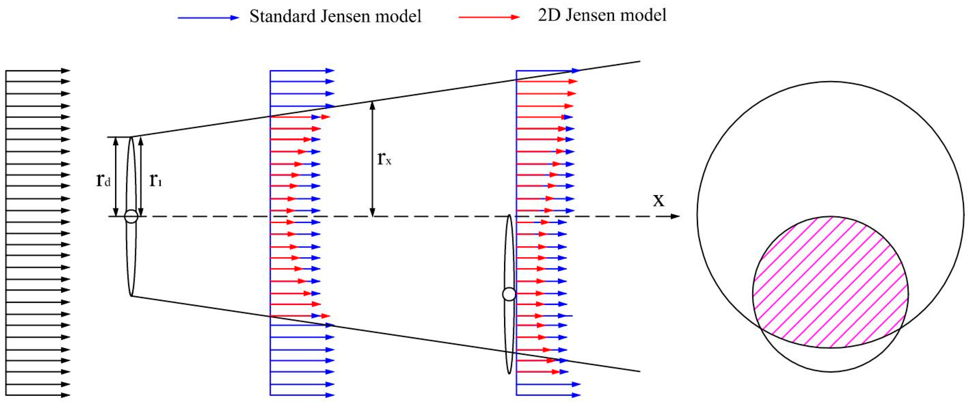
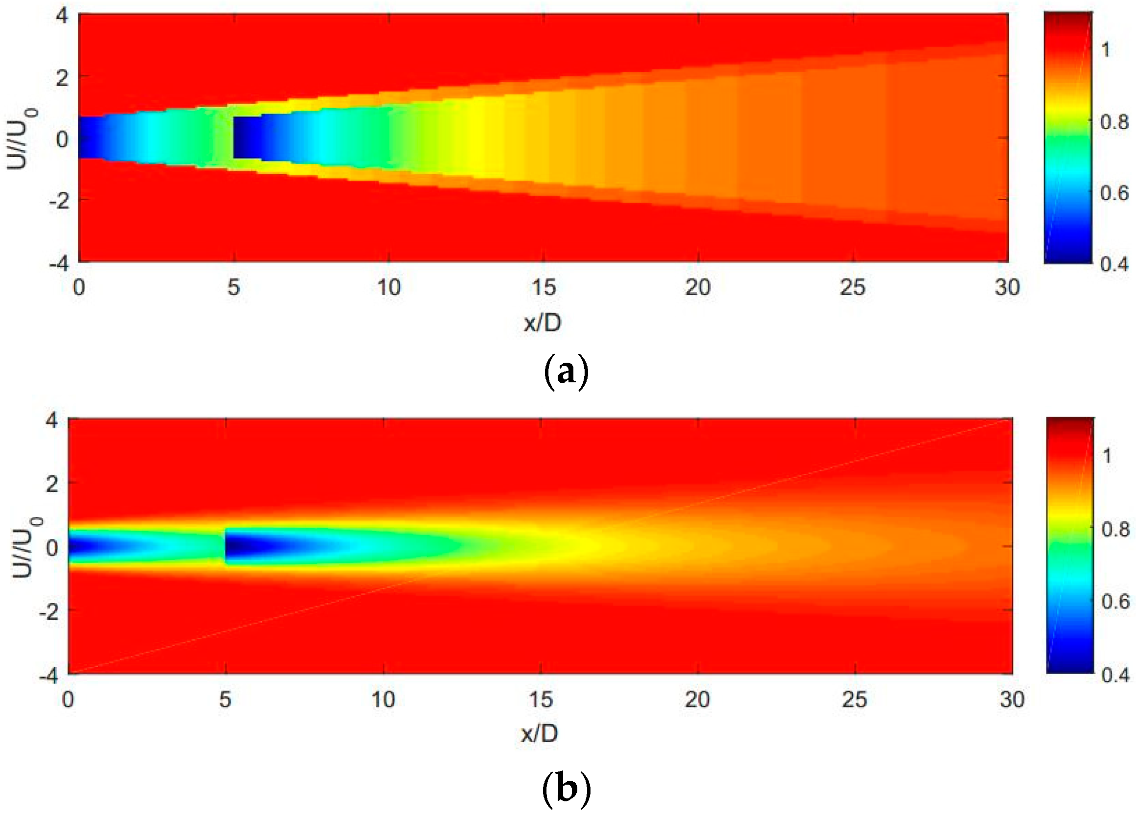
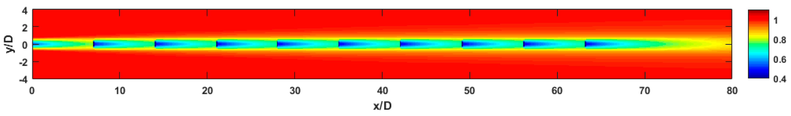
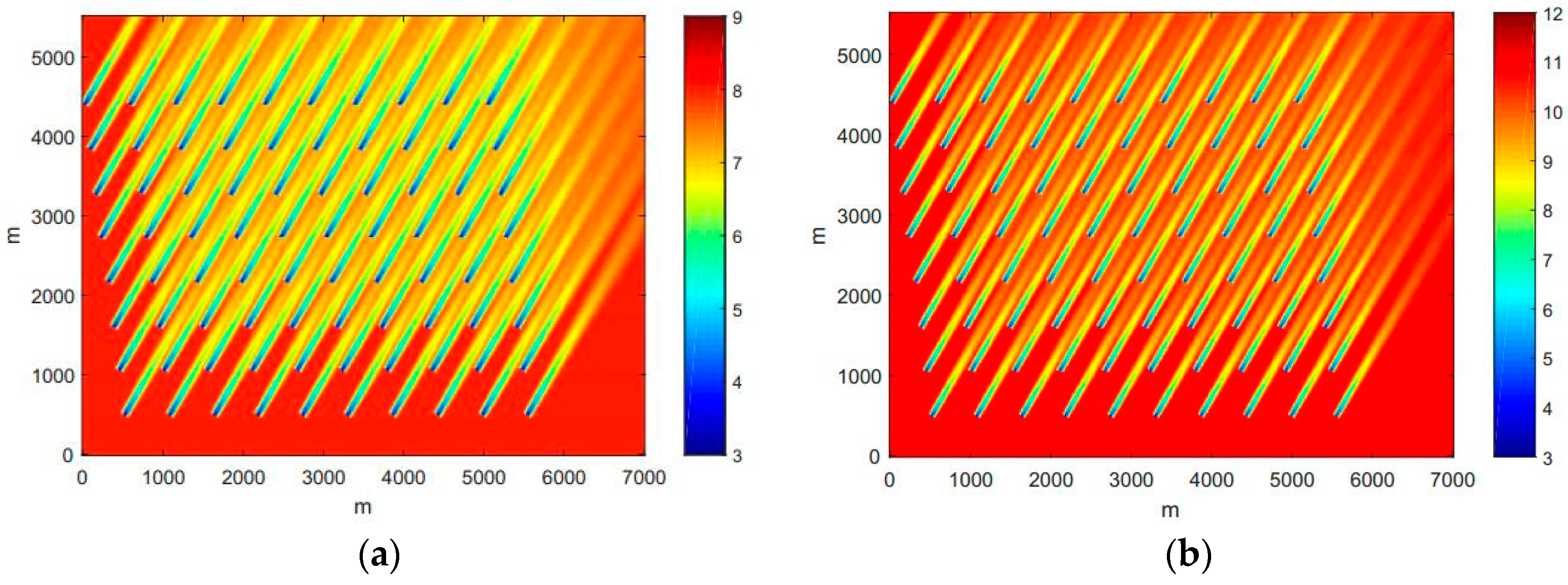
2.1. 2D-Wake Modeling

The standard Jensen’s wake model (1D model) assumes that the wind turbine wake linearly expands with a single parameter which is called the wake decay constant. In reality, the wake of a wind turbine is more complex in wind farms. The wake velocity is known to have nonlinear distribution in different axial section of the wake. To simulate more accurately the wind farm wake distribution, a more accurate 2D wake model considers the effect of turbulence intensity of a wind farm [13,14]. According to this model, the predictor step and corrector step are proposed to calculate the wake velocity in a wind farm as follows:
Predictor step:
u ( x , r ) = u 0 [ 1 2 a ( 1 + k w a k e x / r 1 ) 2 ]
Corrector step:
u ( x , r ) = ( u 0 u ( x , r ) ) cos ( π r r x + π ) + u ( x , r )
where:
a = ( 1 1 C T ) / 2
r x = k w a k e x + r d
r 1 = r d ( 1 a ) / ( 1 2 a )
k 0 = 0.5 / ln ( z / z 0 )
k w a k e = k 0 I w a k e I 0
where a is the axial induction factor calculated from the thrust coefficient CT of the wind turbine; rx is the spread wake radius; rd is the rotor radius of the wind turbine; r1 is the characteristic downstream rotor radius represents the expanded wake radius immediately downstream of the wind turbine; z is the hub height of a local terrain; z0 is the surface roughness height of a local terrain; k0 is the wake decay constant; kwake is the wake decay rate by taking into account the effective wake turbulence; u0 is the wind speed of wind farm; u* is the wake velocity calculated by the standard Jensen’s wake model.
Numerical accuracy of the wake models is essential when the number of wind turbines increases. Figure 1 shows the wake geometry formed by an upwind turbine and a downwind turbine. Depending on the overlapped wake area, three types of wake effects can be observed. As seen the schematic diagram, the velocity profile of the 1D Jensen’s model is ‘hat-shaped’. The modified Jensen’s model reserves the advantage of the original model and allows turbulence to play the role. For the influence of multiple upwind turbines, the velocity deficit due to multiple wakes can be represented as follows:
u ( x , r ) = u 0 [ 1 i = 1 n ( 1 u i ( x , r ) u 0 ) 2 ]
where n is the number of upwind turbines inside the wake of a downwind turbine. The resulting velocity profiles from two wind turbines are shown in Figure 1. Such a wake interaction case is quite representative of a real wind farm, and the overlapped wake area can be estimated using the function mentioned above.

2.2. Wind Turbine Noise Source

For wind turbines in a wind farm, the wind turbine noise sources are different due to the change of wind speed and wind direction. Thus, each wind turbine’s noise spectrum needs to be calculated based on pre-simulated wind farm wake field. It is worth noting that the wind farm noise radiation depends on the farm layout, wind speed, wind directions and turbulence intensity. In order to calculate the aerodynamic noise source generation from wind turbine blades, the semi-empirical wind turbine noise model is applied [16]. At each blade element, the local flow velocities and angles of attack are obtained from the wind farm wake model. The sound pressure level for each segment of blades is calculated based on individual noise mechanisms. Finally, the sound pressure level from each of the individual sources is summed across the blade to calculate the total noise source of the wind turbine.
Based on the aerodynamic noise generation mechanisms, the blade noise sources are separated from turbulent inflow noise and airfoil self-noise. According to Lowson [18], the turbulent inflow noise can be further divided into two frequency regions. For high frequencies, the sound pressure level is given as:
S P L I n f l o w H = 10 log 10 [ D ¯ h ρ 2 c 0 2 L Δ l r 2 M 3 I 2 k ^ 3 ( 1 + k ^ 2 ) 7 / 3 ] + C
For low frequencies, Equation (9) is modified as follows:
S P L I n f l o w = S P L I n f l o w H + 10 log 10 ( K c 1 + K c )
where Kc is a low-frequency correction factor, ρ is the density of air, L denotes the length scale of the atmospheric turbulence, Δl is the airfoil section semi-span, M is the Mach number, I is the turbulence intensity, k ^ is the normalized wave number, and D ¯ h is the effect from sound directivity, c is a correction constant number. Airfoil self-noise is classified into the following five mechanisms:
  • Turbulent Boundary Layer Trailing Edge (TBL-TE) noise, including pressure side and suction side
  • Separation-Stall (SEP) noise
  • Laminar Boundary Layer Vortex Shedding (LBL-VS) noise
  • Tip Vortex Formation (TIP) noise
  • Trailing Edge Bluntness Vortex Shedding (TEB-VS) noise
The blades of the wind turbine are divided into a number of airfoil sections or blade elements. The two-dimensional airfoil self-noise prediction theory is applied for each blade section and the total noise level is determined by summing up all the noise sources. For the ith blade element, the total noise sources are given as follows:
S P L T o t a l i = 10 log 10 ( j 10 0.1 ( S P L j + K A ) )
where j denotes the different noise sources such as inflow noise and airfoil self-noise, KA is the relative response of the A-weighting filter. The TIP noise is not activated except for the blade elements near the tip region. The Sound Pressure Level (SPL) radiated from a single wind turbine is the logarithmic sum of the sound pressure level from all blade elements:
S P L T o t a l = 10 log 10 ( i 10 0.1 S P L T o t a l i )

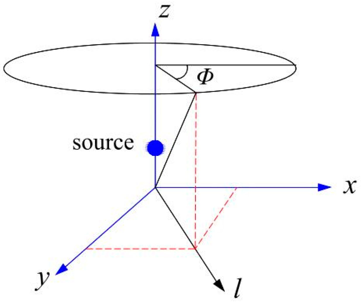
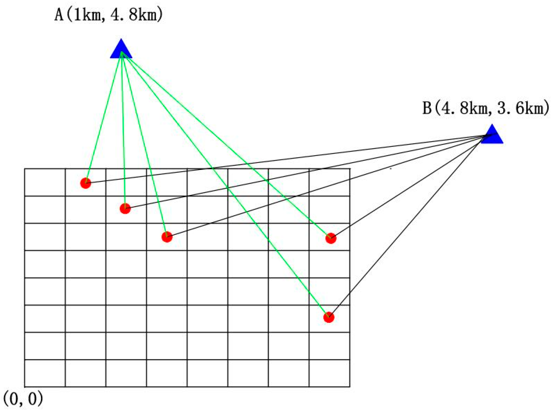
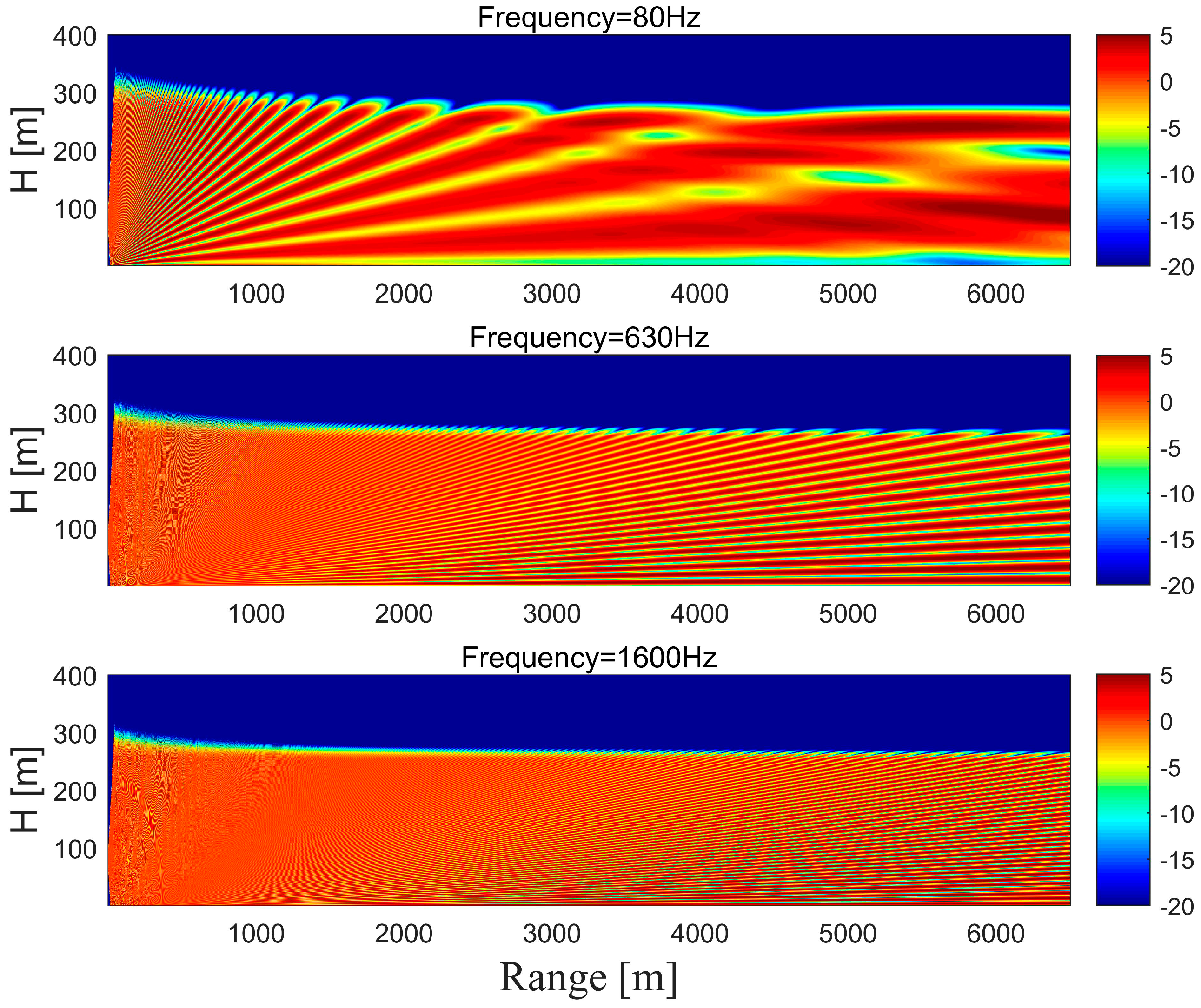
2.3. Wind Turbine Noise Propagation

The Crank-Nicholson PE (CNPE) method [19] is a numerical method that can deal with atmospheric as well as ocean acoustic problems. The method is applied here to simulate the large wind farm noise propagation problem. Based on an axisymmetric approximation, the CNPE method can be simplified into a two-dimensional form. As shown in Figure 2, the noise source is located at a wind turbine hub height, the simulations are then carried out in the 2D domains.
In the axisymmetric approximation we neglect the variation of the sound field with the azimuthal angle ø. Such an approximation implies that the 3D Helmholtz equation can be reduced into the 2D Helmholtz equation as:
2 q c l 2 + 2 q c z 2 + k e f f 2 q c = 0
where the quantity qc in Equation (13) is related to the complex pressure amplitude pc such as:
q c = p c l
keff is the effective wave number such that keff = ω/Ceff, where ω is the angular frequency and Ceff is the effective sound speed.
We can also write the solution of Equation (14) as:
q ( l , z ) = ψ ( l , z ) exp ( i k a l )
where ka is the value of the wave number kz is the wave number defined at some average height or at the ground surface. The factor exp(ikal) represents a plane wave traveling in the positive l direction, and oscillates rapidly as a function of l; the function ψ(l,z) usually varies slowly with the distance l.
Inserting Equation (15) to Equation (13), we obtain the parabolic equation:
2 i k a ψ l + 2 ψ l 2 + ( k e f f 2 k a 2 ) ψ = 0
Solving the PE using the Crank-Nicholson approach, we will have the attenuation of sound propagation, which is defined as ΔL in this paper. It represents sound pressure deviations such as ground reflection, atmospheric refraction, atmospheric turbulence, irregular terrain and noise barriers.
The previously calculated wind turbine sound power level Lw(f) is the initial condition for calculating long range noise propagation. At each frequency, sound propagation loss is computed as:
L p ( f ) = L w ( f ) 10 log 10 4 π D 2 α D + Δ L
Here Lw(f) is an integrated value of Lp(f) which is the measure of sound power level, and it does not change with distance. The term 10 log 10 4 π D 2 is the geometric attenuation corresponds to spherical spread of sound waves from the source. The effect from atmospheric absorption is calculated with the term D. The attenuation is proportional to the propagation length D, the coefficient α corrects the air absorption at different frequency, temperature, pressure and humidity. In the present simulations, a relative humidity of 70% and a temperature of 10 °C are used as default condition. Thus, at a given receiver location, we can get the total noise spectrum by superimposing the noise levels from n wind turbines that arrive at a receiver r:
L l ( f ) = 10 log 10 ( i = 1 n L p i ( f ) )
Figure 3 is a top view showing the noise propagation paths from different wind turbines towards given receivers. As shown in the figure, A and B are the two noise exposed areas (villages) nearby a small wind farm. The total noise arrived at the villages is the combined effect from all wind turbines. The noise source spectrum Lp is first obtained using a noise source model. In the next step, using Equation (18), the overall noise level at A and B is the SPLs summed up at each frequency. Repeating the procedure at all the prescribed mesh points forms the noise map in the wind farm area.

3. Numerical Results

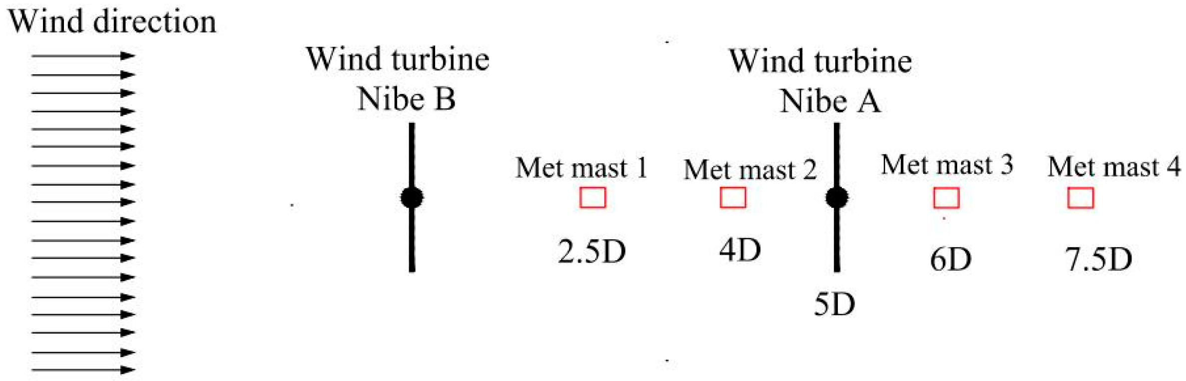
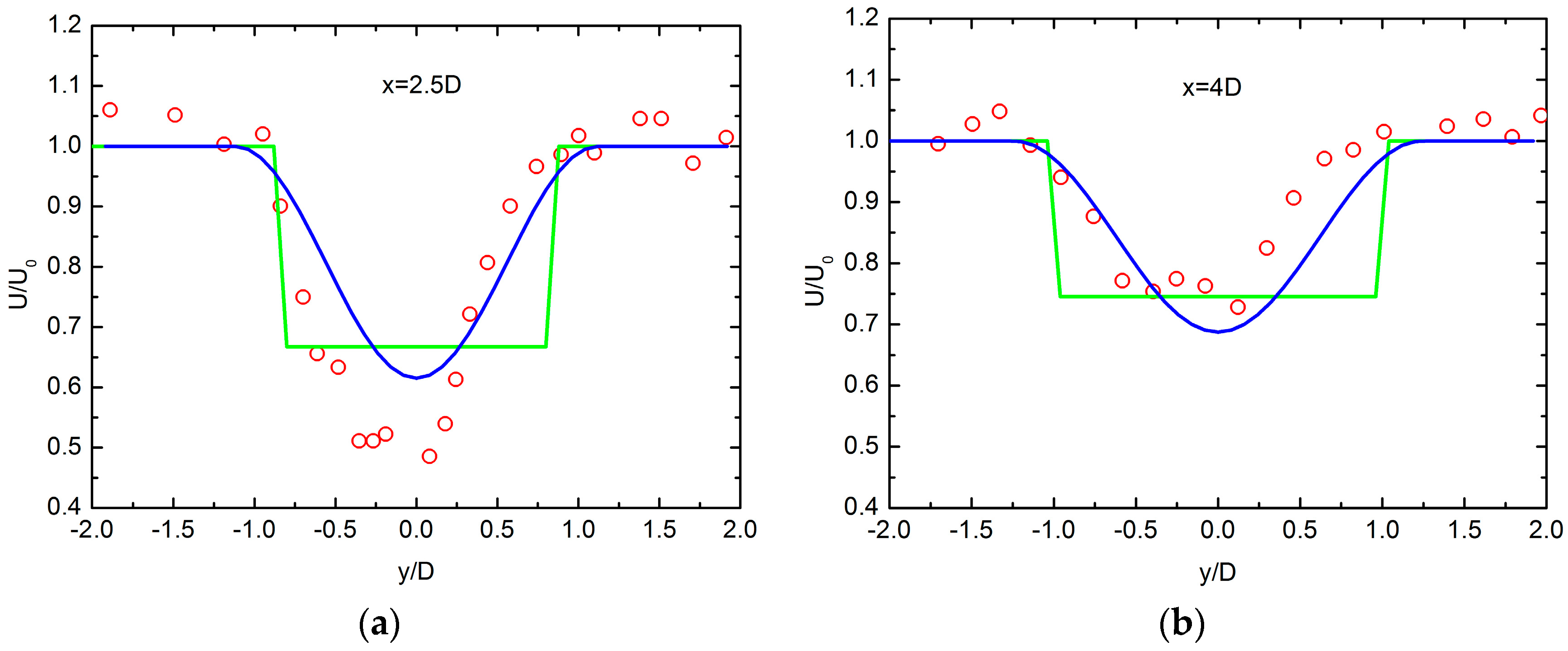
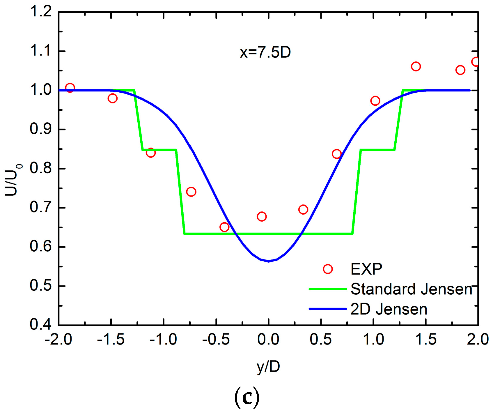
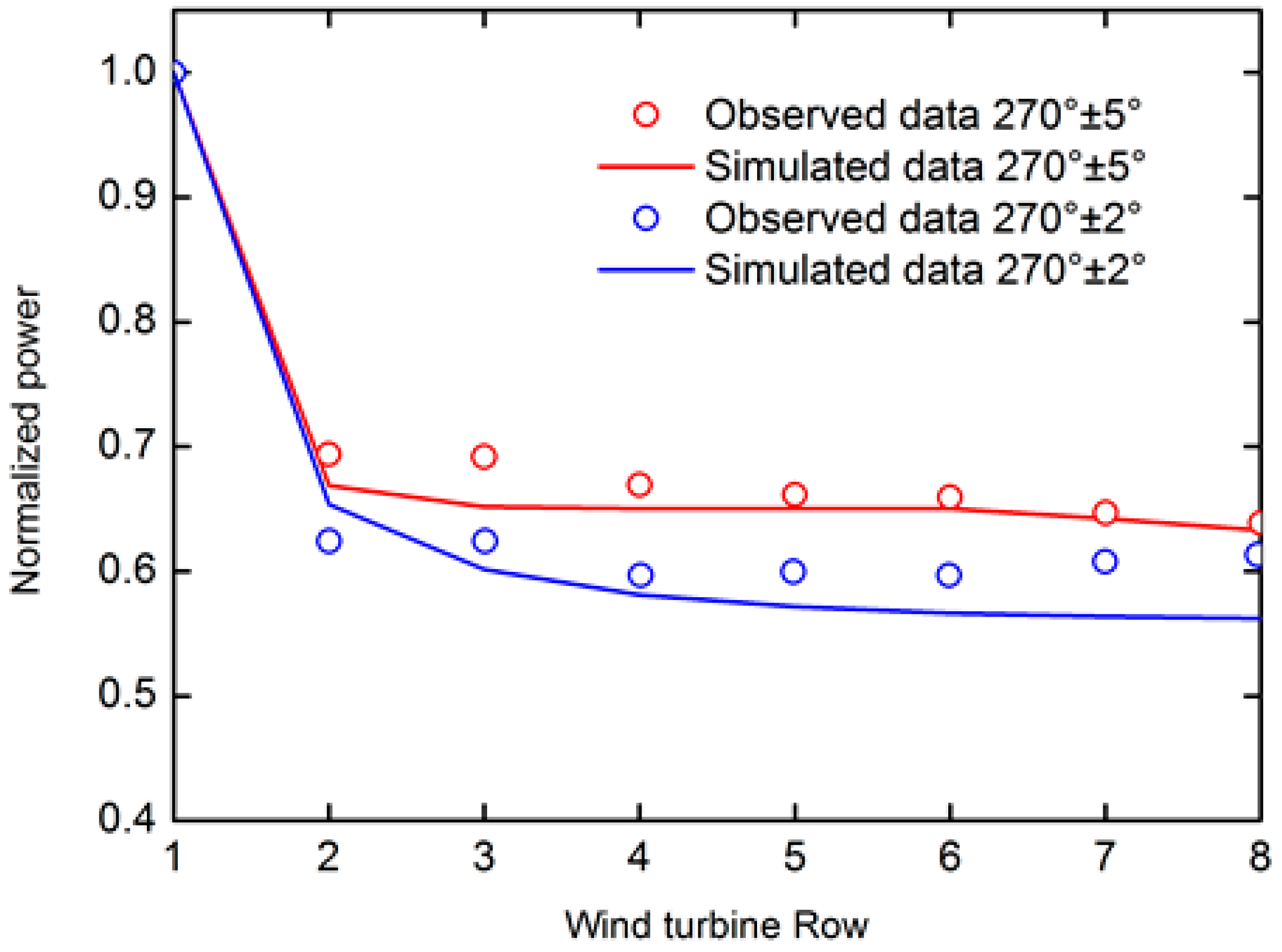
3.1. Wake Modeling Validations

In this section, the aerodynamic model accuracy is first validated with a field experiment. The full-scale measurements [20] of the Nibe wind turbines are illusitrated in Figure 4. There are four meteorological masts (M1, M2, M3, M4) placed at different downstream positions (2.5D, 4.0D, 6.0D, 7.5D) with respect to the Nibe B wind turbine. The two turbines are seperated with an axial distance of 5 rotor diameters (5D). The rated power of the wind turbines is 630 kW; the rotor diameter of the Nibe wind turbine is D = 40 m; the hub height is H = 45 m. The simulation was carried out at wind speed of 8.55 m/s, a surface roughness length 0.1m, a thrust coefficient Ct 0.82 and a turbulence intensity of 10%. The measured velocity data are recorded for two wind turbines at down-stream positions of 2.5D, 4.0D and 7.5D as seen in Figure 4.
Based on the different wake models used, the streamwise velocity contour plot is presented in Figure 5 for the double wind turbines. Figure 5a is the result obtained from standard Jensen’s model, Figure 5b is the result of the 2D Jensen’s model. The results from both models show that the axial velocity is largely reduced when the axial flow first passes through the Nibe B wind turbine. The Nibe A wind turbine futher extracts energy from the wake of Nibe B, wake recovering is seen after Nibe A. The improved Jensen’s wake model is designed with a 2D wake profile, it shows that the 2D wake model is closer to the measured data. The comparisons between the measured and simulated wake profiles for two wind turbines at down-stream positions of 2.5D, 4.0D and 7.5D are shown in Figure 6. At a distance of 2.5D, the wake velocity is slightly over estimated by both wake models. As expected, the 1D Jensen’s model predicted a constant wake velocity at the distances of 2.5D and 4.0D. For the results obtained from the improved Jensen’s wake model, the wake velocity at the same distances are more closely matched with the measured wake profiles. Figure 6c shows a more complicated double wake case where the wake flow of the two wind turbines is superimposed. At a distance of x = 7.5D, the wake velocity is further reduced due to the presence of the Nibe A wind turbine. The 1D Jensen’s wake model shows the wake expansion with two separate velocities which does not occur in reality. The improved model shows a strong mixing of the two wake flows which better matches the measured wake profile.

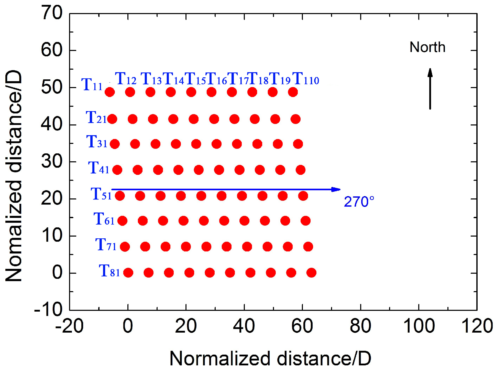
3.2. Horns Rev Wind Farm Case

In order to predict and analyze noise distribution of a large wind farm, the Horns Rev wind farm is simulated in different wind directions and wind speeds, such that the flow field is prepared as input to noise propagation study. The Horns Rev offshore wind farm is located in the eastern North Sea off Denmark. The wind farm consists of the V80-2MW wind turbines within an occupied area of about 20 km2. The farm layout is shown in Figure 7. The wind turbines are arranged in a skewed rectangular array of 8 by 10 turbines. Such a regular layout fits very well for purpose the present wake and noise investigations. The wind turbines in the Horns Rev wind farm are placed with an internal spacing along the main directions of 7D. The wind turbines have a hub height of 70 m, a rotor diameter of D = 80 m, and a rated rotational speed of 18 rpm. The cut-in wind speed is 5 m/s; the rated wind speed is 12 m/s; the cut-out wind speed is 20 m/s. The detailed pitch angle, rotational speed and blade geometry data are provided from the reference paper [5]. The rotor blade is composed of the NACA63-series airfoils between the blade tip and the mid-span, the FFA-W3-series airfoils are used between the mid-span towards blade inboard part. The simulations are performed with a surface roughness length 0.005 m. The north and west wind directions are defined as 360° and 270°, as depicted in Figure 7.
With the rotor geometry and wind conditions provided above, a typical normalized power performance along the 270° wind direction is simulated and compared with measure power. The measured data contains wind direction uncertainty, such as 270° ± 2° and 270° ± 5°. A fair comparison is thus carried out under the same conditions. According to the measured and simulated data, there is a quite large power deficit seen from the second row of wind turbine, as shown in Figure 8. It will be shown later that the change of sound pressure level is not as much as the mechanical power does.

3.2.1. Noise Propagation from a Single Wind Turbine

We start the long range noise propagation simulation from a single V80 wind turbine. Firstly, the aerodynamic noise sources are simulated at different inflow wind speed conditions. When inflow wind speed is 12 m/s, the wind turbine aerodynamic noise spectra are shown in Figure 9a. As introduced before, the total sound pressure level (SPL-total) is obtained by summing up all the noise sources. In the present case, the SPL is recorded on the ground level with a horizontal distance of 110 m which equals to the tower height plus blade length. The sound power level is a measure of sound power strength which does not change with distance. Figure 9b shows sound power spectra at various wind speeds. The sound power spectra are A-weighted to correct the sensitivity of human ear. It is seen that the difference in dB level at various wind speed is obvious, but not as significant as the variation in mechanical power, as previously discussed in Figure 8. The reason is that the change of sound pressure level follows log-law, for example, double the sound pressure only result an increase in SPL about 3 dB.
Figure 10 shows the attenuation of sound pressure (ΔL) during propagation with the range and height. The noise source is placed at the hub height. The absorption layer is set on top of the domain such that the radiated noise is not reflected back into the domain. The reflected waves from ground are superimposed with the direct waves which show different characteristics at different frequencies. At f = 80Hz, 630 Hz and 1600 Hz, when the wavelength becomes smaller, the higher resolution of the mesh is required to capture high frequency wave propagation.

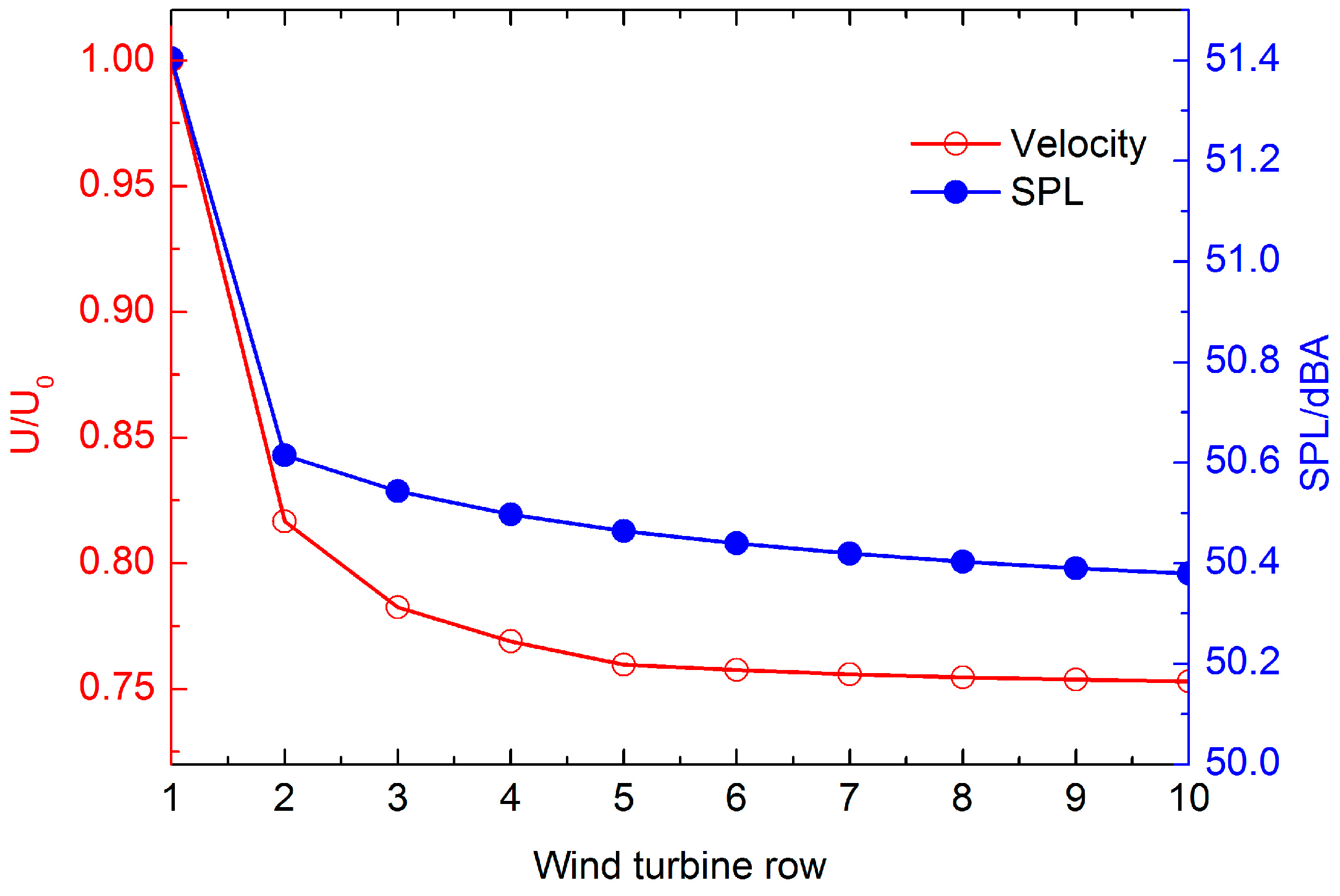
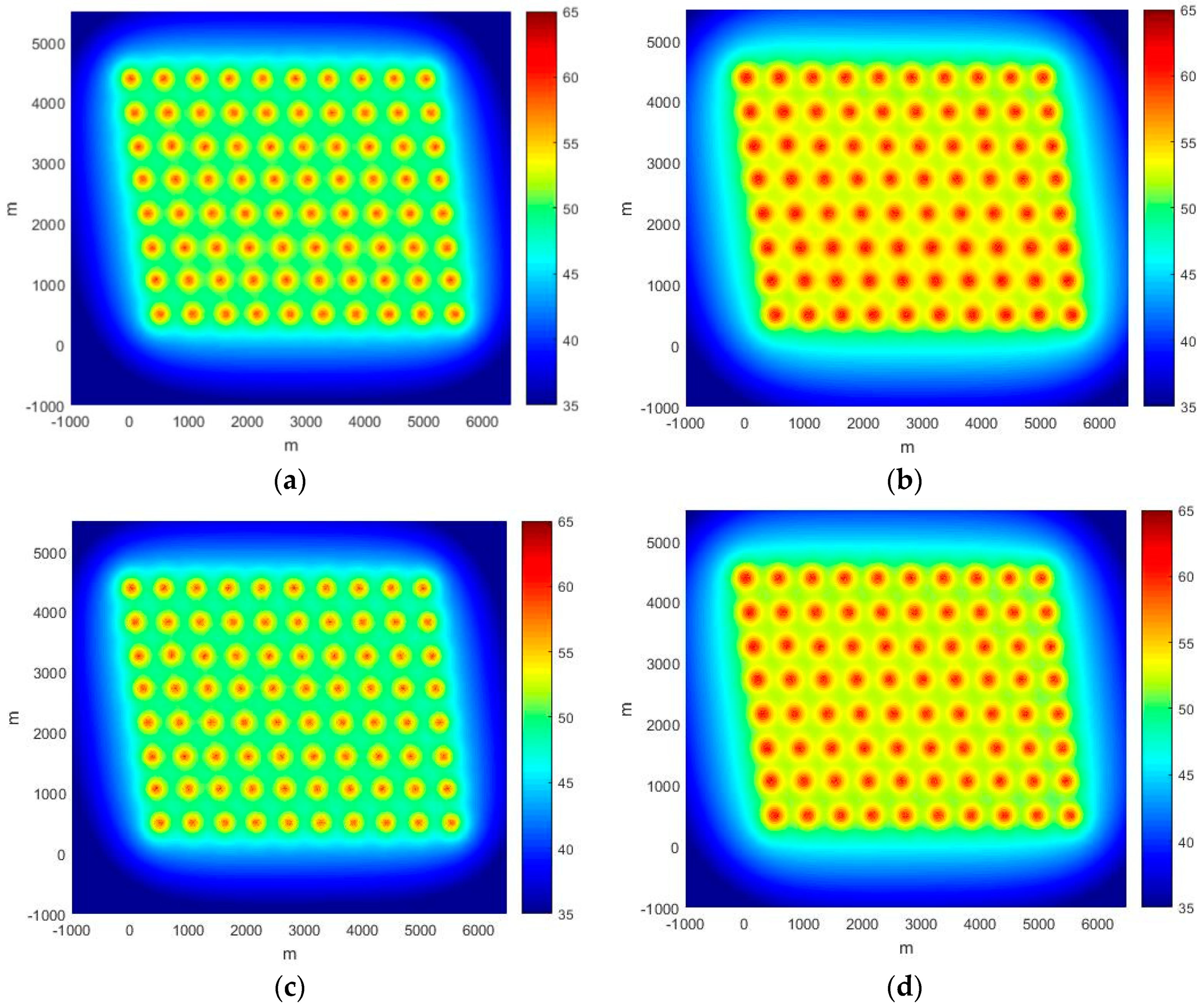
3.2.2. Multiple Wind Turbine Noise

As an example of flow through multiple wind turbines, a simulation is shown for flow through 10 wind turbines at a wind speed of 12 m/s, with a roughness length of 0.005 m, a thrust coefficient Ct 0.689 and a turbulence intensity of 6.9%. Figure 11 shows the normalized horizontal velocity contours along the multiple wind turbines in a row. The spacing of each wind turbine is 7D that is the same case of the depicted 270° wind direction in the Horns Rev wind farm. The amount of wind energy extracted from the wind turbines is seen by the wake deficit where the wake velocity continuously decreases along the row. In Figure 12, the normalized flow velocity is shown together with the SPL of each wind turbine. The same trend is found that both the velocity and SPL drops significantly from the second wind turbine and the other wind turbines in the wake. However, the figure shows that the changes of dB in percentage are much less than that of velocity changes.

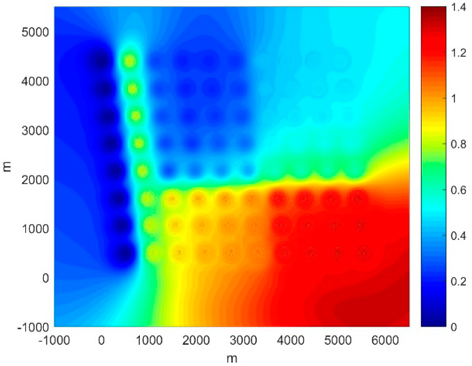
3.2.3. Offshore Wind Farm Noise

For a more general case, we consider flow and acoustic radiation in a realistic wind farm. Although noise radiation from such an offshore wind farm is not an issue at least for human beings, but the numerical method presented here can be extended to onshore wind farms. Two inflow wind speeds are considered at 8 and 11 m/s. The roughness length is 0.005 m, thrust coefficients are Ct = 0.689 and 0.81 at two wind speeds, respectively, the turbulence intensity is 6.9%. Figure 13 presents the wake velocity in the different wind directions and inflow wind speeds. Very large wake blockage is seen in the direction of 270° compared with the direction of 210°. This indicates the large amount of energy lost when the wind turbines are aligned. As compared with the power efficiency with the first upstream wind turbine, the performance of the wind turbines in the wake is reduced up to 60%–70% of the reference wind turbine.
In Figure 14, the corresponding aerodynamic noise map is shown at four wind conditions. The overall sound pressure level is calculated in an area over 48 km2. At each mesh point of the computational domain, the overall SPL is the logarithmic summation of the SPL received from individual wind turbines. In Figure 15, the ΔSPL between two wind directions is shown for the 11 m/s case.

4. Discussions

The numerical results are shown in the previous section. Firstly, the wake flow of a single wind turbine (Nibe B) and a double wind turbine (Nibe A and B) are simulated and compared with the measured data. The improved Jensen’s wake model [13,14] is shown superior to the original model [2]. Secondly, the aerodynamic simulation is extended to the Horns Rev wind farm. A large power variation is observed when the wind turbines are clustered. Thirdly, the wind turbine noise source is simulated based on the computed velocity distributions. It is observed that wind velocity continuously decreases along the wind turbine cluster, so does the noise generation from each wind turbines in the cluster. Finally, as a most important output from the study, the wind farm noise maps are computed in a wide range using the parabolic equation method [17]. As previously seen in Figure 3, in the present wind farm case, the number of noise propagation simulation is Nt × Nf where Nt is number of wind turbines and Nf is number of selected frequencies in a 1/3-octave band. The change of noise level at the wind speeds of 8 m/s and 11 m/s, was shown in Figure 9b. As a result, higher SPL distribution around the wind farm is found at higher wind speed. From the contour levels shown in Figure 14, it is clear that both wind speed and wind direction affect the noise distribution around a wind farm. Also, as previously shown in Figure 10, the characteristics of noise propagation from the source are different at each frequency. The noise spectra of the wind turbines behind the first row are all different. This is more obvious by comparing Figure 14b with Figure 14d where wind speed is the same but the inflow angle changes from 210° to 270°. In a conventional approach, if one only considers noise generation and propagation from a single wind turbine, the SPL nearby the first row (T11, T21, …, T81 in Figure 7) should be the same for case (a), (b) and case (c), (d), respectively. In the present simulations, the propagation of noise source plays an important role. Some observations are found from Figure 14 and Figure 15: (1) although the source level are the same for the first row (due to the same inflow condition), but the ΔSPL is not zero because of the propagation effect from the downward wind turbines; (2) the second row shows more pronounced differences in SPL because of the much larger velocity deficit in the direction of 270°; (3) in the direction of 210°, in the lower right corner the wind farm generated higher noise comparing to the case of 270°. The simulations prove that higher power production corresponding to higher noise radiation which is seen as a contradiction for wind farm planning. The most recent and relevant work that studies long range wind turbine noise propagation is given by Dietrich et al. [21]. The noise propagation in the downstream domain of the wind turbine is influenced by the slope of a hill. While in the present simulations, we only consider flat terrain with large number of wind turbines. The ray theory is often used for long range sound propagation study [21]. The method based on ray theory is a high-frequency approach such that low-frequency results are not very accurate in the cases of strong refraction and diffraction. The present numerical approach is more expensive. The PE method directly solves the wave equation which is also frequency dependent. To solve high frequency sound propagation problems, a higher grid density is required, thus increasing the computational time.

5. Conclusions and Future Work

The paper combined two issues: wind farm power prediction and noise evaluation. In the past, maximum power generation with lowest cost is no doubt the only factor that was considered during wind farm planning. The related power prediction methods were intensively studied which can be found in many references. It is not the main focus of the present paper to evaluate in much detail the wake prediction models or the optimization algorithms. Based on our previous investigations, an improved Jensen’s model was selected for purpose of wind farm aerodynamic simulations. The method is proven to be efficient and it represents more physics of the wake profile. The connection of wind farm wake and the noise propagation is through the wind turbine noise source prediction. The rotor aerodynamic noise sources are characterized by a few noise mechanisms, they are all related to wind speed, wind direction and turbulence intensities in the wind farm, such that different wind farm layout yields different wind farm noise map. The present study was carried out for an operating wind farm with a fixed layout. Unlike the wind resource map, the resulting noise map is thus not unique, each noise map corresponds to a specific flow condition which is further related to machine characteristics, such as rotor aerodynamic shape, rotational speed and pitch settings etc. Wind farm noise can be controlled at several stages: (1) rotor design stage: achieve low noise airfoil and blade design; (2) aftermarket stage: add passive noise reduction devices, such as trailing edge serration; (3) wind farm construction stage: achieve an optimal layout with low noise emission and high energy efficiency; (4) wind farm operation stage: smart control of rotational speed and pitch settings in the circumstances of too high noise emission. Based on this study, it can be shown that a more comprehensive work can be performed with the aim of modeling wind farms under planning. With a low aerodynamic noise designed machine and optimized farm layout, it is expected that future development wind farms will be both more cost efficient and more environmentally friendly.

Author Contributions

W.Z. conceived the method and wrote most part of the paper; J.C. carried out most of the programming part and the simulations was partly carried out by X.W.; T.W. and H.X. put efforts on comments and discussions.

Funding

This work was funded by the Jiangsu Province Natural Science Foundation (BK20160476), the National Science Foundation (11672261), and the Yangzhou University Science and Technology Innovation Training Foundation (2017CXJ041), the Natural Science Research Projects of Colleges and Universities in Jiangsu Province (16KJB480003), and the Jiangsu Province Natural Science Foundation (BK20170510).

Acknowledgments

The corresponding author wish to express special acknowledgement to the National Nature Science Foundation for funding under grant number 11672261, and the Jiangsu Province Natural Science Foundation (BK20160476).

Conflicts of Interest

The authors declare no conflict of interest.

References

  1. Andersson, M. Offshore Wind Farms Ecological Effects of Noise and Habitat Alteration on Fish; Stockholm University: Stockholm, Sweden, 2011. [Google Scholar]
  2. Gocmen, T.; Van der Laan, P.; Rethore, P.-E.; Diaz, A.P.; Larsen, G.C.; Ott, S. Wind turbine wake models developed at the technical university of Denmark: A review. Renew. Sustain. Energy Rev. 2016, 60, 752–769. [Google Scholar] [CrossRef] [Green Version]
  3. Mikkelsen, R. Actuator Disc Methods Applied to Wind Turbines; MEK-FM-PHD 2003-02; Technical University of Denmark: Lyngby, Denmark, 2003. [Google Scholar]
  4. Sørensen, J.N.; Shen, W.Z.; Munduate, X. Analysis of wake states by a full-field actuator disc model. Wind Energy 1998, 1, 73–88. [Google Scholar] [CrossRef]
  5. Wu, Y.-T.; Porté-Agel, F. Modeling turbine wakes and power losses within a wind farm using LES: An application to the Horns Rev offshore wind farm. Renew. Energy 2015, 75, 945–955. [Google Scholar] [CrossRef]
  6. Shen, W.Z.; Zhu, W.J.; Sørensen, J.N. Actuator line/Navier-Stokes computations for the MEXICO rotor: Comparison with detailed measurements. Wind Energy 2012, 15, 811–825. [Google Scholar] [CrossRef]
  7. Troldborg, N.; Larsen, G.C.; Madsen, H.A.; Hansen, K.S.; Sørensen, J.N.; Mikkelsen, R. Numerical simulations of wake interaction between two wind turbines at various inflow conditions. Wind Energy 2010, 14, 859–876. [Google Scholar] [CrossRef]
  8. Ciri, U.; Petrolo, G.; Salvetti, M.V.; Leonardi, S. Large-Eddy Simulations of Two in-line Turbines in a Wind Tunnel with Different Inflow Conditions. Energies 2017, 10, 821. [Google Scholar] [CrossRef]
  9. Frandsen, S. On the wind speed reduction in the center of large clusters of wind turbines. J. Wind Eng. Ind. Aerodyn. 1992, 39, 251–265. [Google Scholar] [CrossRef]
  10. Jensen, N.O. A Note on Wind Generator Interaction; Risø-M-2411 Risø National Laboratory Roskilde: Roskilde, Denmark, 1983; pp. 1–16. [Google Scholar]
  11. Larsen, G.C.; Madsen, H.A.; Thomsen, K.; Larsen, T.J. Wake meandering: A pragmatic approach. Wind Energy 2008, 11, 377–395. [Google Scholar] [CrossRef]
  12. Herbert-Acero, J.F.; Probst, O.; Rethore, P.E.; Larsen, G.C.; Castillo-Villar, K.K. A Review of Methodological Approaches for the Design and Optimization of Wind Farms. Energies 2014, 7, 6930–7016. [Google Scholar] [CrossRef] [Green Version]
  13. Tian, L.; Zhu, W.; Shen, W.; Zhao, N.; Shen, Z. Development and validation of a new two-dimensional wake model for wind turbine wakes. J. Wind Eng. Ind. Aerodyn. 2015, 137, 90–99. [Google Scholar] [CrossRef] [Green Version]
  14. Tian, L.; Zhu, W.; Shen, W.; Song, Y.; Zhao, N. Prediction of multi-wake problems using an improved Jensen wake model. Renew. Energy 2017, 102, 457–469. [Google Scholar] [CrossRef]
  15. Brooks, T.F.; Pope, D.S.; Marcolini, M.A. Airfoil Self-Noise and Prediction; National Aeronautics and Space Administration: Washington, DC, USA, 1989.
  16. Zhu, W.J.; Heilskov, N.; Shen, W.Z.; Sørensen, J.N. Modeling of Aerodynamically Generated Noise from Wind Turbines. J. Sol. Energy Eng. 2005, 127, 517–528. [Google Scholar] [CrossRef]
  17. Salomons, E.M. Computational Atmospheric Acoustics; Springer Sciences & Bussiness Media: Berlin, Germany, 2012. [Google Scholar]
  18. Lowson, M.V. Assessment and Prediction of Wind Turbine Noise; Flow Solutions Report 92/19, ETSU W/13/00284/REP; Energy Technology Support Unit: Harwell, UK, 1993; pp. 1–59.
  19. West, M.; Gilbert, K.; Sack, R.A. A tutorial on the parabolic equation (PE) model used for long range sound propagation in the atmosphere. Appl. Acoust. 1992, 37, 31–49. [Google Scholar] [CrossRef]
  20. Taylor, G.L. Wake Measurements on the Nibe Wind Turbines in Denmark; National Power-Technology and Environment Center: Leatherhead, UK, 1990. [Google Scholar]
  21. Heimann, D.; Englberger, A.; Schady, A. Sound propagation through the wake flow of a hilltop wind turbine—A numerical study. Wind Energy 2018, 21, 650–662. [Google Scholar] [CrossRef]
Figure 1. Schematic diagram of wake velocity for multiple wind turbines.
Energies 12 00018 g001
Figure 2. Rectangular x-y-z coordinates and cylindrical l-ø-z coordinates.
Energies 12 00018 g002
Figure 3. Schematic diagram of wind turbine noise source propagations towards receiver.
Energies 12 00018 g003
Figure 4. Schematic diagram of the Nibe wind turbines and the wake measurement locations (Top view).
Energies 12 00018 g004
Figure 5. Contours of the wake velocity for two Nibe wind turbines. (a) Standard Jensen’s model; (b) 2D Jensen’s model.
Energies 12 00018 g005
Figure 6. Comparisons between the measured and simulated wake velocity data of two wind turbines at down-stream positions of (a) 2.5D, (b) 4.0D and (c) 7.5D.
Energies 12 00018 g006aEnergies 12 00018 g006b
Figure 7. Layout of the Horns Rev wind farm.
Energies 12 00018 g007
Figure 8. Comparisons of normalized power in the direction of 270°.
Energies 12 00018 g008
Figure 9. The wind turbine noise source (a) sound pressure level, 12 m/s; (b) sound power level with the different inflow wind velocity, 5 m/s, 8 m/s, 11 m/s, 12 m/s.
Energies 12 00018 g009
Figure 10. Relative sound pressure level at different frequencies.
Energies 12 00018 g010
Figure 11. Contours of the wake velocity for 10 wind turbines.
Energies 12 00018 g011
Figure 12. Wake velocity and SPL with wind turbine row.
Energies 12 00018 g012
Figure 13. Wake velocity of Horns Rev wind farm in different wind direction and speed. (a) 210°, 8 m/s; (b) 210°, 11 m/s; (c) 270°, 8 m/s; (d) 270°, 11 m/s.
Energies 12 00018 g013aEnergies 12 00018 g013b
Figure 14. Sound pressure level of Horns Rev wind farm in different wind direction and speed. (a) 210°, 8 m/s; (b) 210°, 11 m/s; (c) 270°, 8 m/s; (d) 270°, 11 m/s.
Energies 12 00018 g014
Figure 15. The SPL differences at 11 m/s, SPL210o-SPL270o.
Energies 12 00018 g015

