Experimental Analysis on Flame Flickering of a Swirl Partially Premixed Combustion

Abstract

An experiment was conducted to explore the flickering parameters under varying mass flow rate of fuel $\dot{m}$_F with spatial analysis and global analysis. The parameters include mean value, flickering weighted average frequency F, flickering coefficient of variation c_v (firstly introduced), skewness s, and kurtosis k. From the spatial analysis, it was found that the brightest part of flame is located in its core, and the brightness gradually decreased from the inside out. The distributions of high levels of F, c_v, s, and k are almost consistent, all lying in the flickering edge, which is a thin layer where the parameters sharply declined. From the global analysis, with the increment of $\dot{m}$_F, the global F decreased slightly; the global c_v declined uniformly, which means the oscillation amplitude diminished and thus the flame became more stable; the global s linearly reduced; and the global k also showed a decreasing trend. The decreasing global s indicates that the number distribution gradually became symmetric, and the decreasing global k indicates that the number distribution progressively became flat. Consequently, the number distribution progressively tends to normal distribution at larger $\dot{m}$_F.

1. Introduction

As can be observed in many combustion processes, flame always exhibits an oscillatory behavior at any moment, and flame structure changes randomly even under stabilized supplies of fuel and oxidizer. This phenomenon is usually entitled as flame flickering, flame puffing, or flame pulsation [1]. It is triggered by large vortices moving around the flame surface owing to buoyancy, which is known as the Kelvin–Helmholtz instability [2]. Flame flickering plays a significant part in combustion properties, such as combustion efficiency, flame size, flame radiation, and air entrainment. Under the acute cases, flame extinction and device failure can be induced due to the oscillation. It is, therefore, essential to understand the flame flickering for better control of combustion [3].

In recent decades, numerous studies have been carried out on the characteristics of flame flickering, primarily under diffusion flame. Bahadori et al. [4] and Durox et al. [5] explored influence of gravity level g on flickering frequency f. They discovered a relationship of power function between f and g respectively, that is, f ∝ g^0.5 from the former but f ∝ g^0.67 from the latter. Arai et al. [6] explained that the increment in f at larger g is the result of the increase in wave velocity and decrease in wavelength. The effects of burner diameter d on f were studied by different investigators, they proposed a consistent model as f = Cd^−0.5 [7], while C is constant but varying among various experiments. For instance, C is 1.5 in Cetegen and Kasper [8], 1.68 in Malalasekera et al. [1], 1.52 in Pagni [9], and 1.73 in Bejan [10].

Yilmaz et al. [11] performed an in-depth visual analysis to oscillatory flame by acquiring flow field oscillation during the flickering process using particle image velocimetry (PIV). Yilmaz et al. [12] used a light sensitive device named cadmium sulfide photocell to measure the variation in light resulted from flame pulsation, suggesting that the mechanisms responsible for flame pulsation are strongly dependent on burner configuration. Pan et al. [2] performed an experiment to examine the flickering behavior of a bluff-body, and found that flickering frequency gradually enlarges with the rising flow velocity of the annular air. Tang et al. [13] explored puffing frequency under varying aspect ratio of rectangular burner; the results revealed that the frequency amplified as the aspect ratio increased. Gotoda et al. [14] measured the pulsation frequency and amplitude of flame tip under various concentrations of oxygen. It was concluded that, with the increment in oxygen concentration, the frequency increases monotonically while the amplitude reduces sharply. Fang et al. [15] experimentally analyzed the flickering characteristics under different air pressure (less than atmosphere). They pointed out that the pool fire at low air pressure is more buoyant, resulting in a larger flickering frequency and stronger oscillation level. In addition, other experiments conducted in sub-atmospheric conditions can also be found in other studies [16,17], and those conducted in a confined compartment can be seen in various studies [18,19,20].

Moreover, serval studies on flame flickering of premixed flames were performed. Kostiuk and Cheng [21] observed the flickering under normal gravity g, microgravity, and reverse gravity (-g), reporting that the root cause behind the puffing is the buoyant force. Gotoda et al. [22] explored the pulsation of flame structure using methane–air mixture and propane–air mixture, respectively, as fuels; they found that the flame oscillation occurs only when the Lewis number of the mixture is higher than one. Durox et al. [23] studied the oscillating behavior of premixed flames under varying pressure, flow velocity, and equivalence ratio. Fujisawa et al. [24] examined the influence of co-flow on flame flickering and concluded that the pulsation frequency increases and amplitude declines with the increase in the velocity of co-flow, while the amplitude enlarges as the equivalence ratio grows.

This section briefly summarized the studies on flame flickering under diffusion flames and premixed flames. However, little work has been reported on the flickering characteristics of partially premixed flame, which has been widely applied in numerous combustion devices because of its high stability. The partially premixed flame is generated when a sub-stoichiometric portion of air (as also named primary air) is premixed with the fuel before combustion, and the mixture burns with an initially separated secondary air [25].

The aim of this work is to analyze the flickering behavior in a partially premixed combustor by conducting an experiment under varying mass flow rate of fuel. Using image processing methodology, for each case, we performed a spatial analysis and global analysis to five parameters. These parameters included mean value, flickering weighted average frequency, flickering coefficient of variation, skewness, and kurtosis. The present analysis exerts an effect to provide more detailed information on flame flickering of partially premixed combustion.

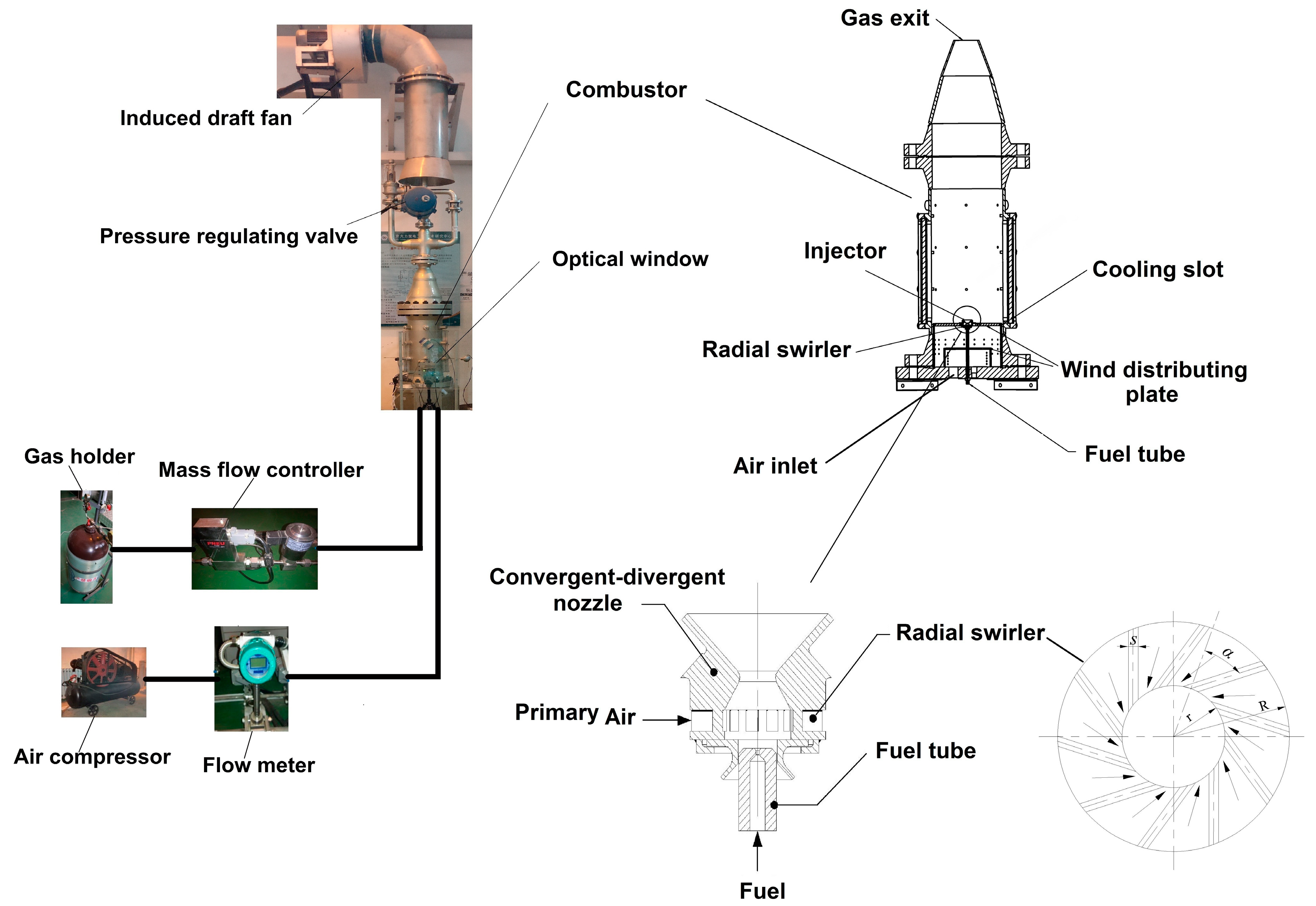
2. Experimental Setup

For this investigation, a combustion test rig was installed, as shown in Figure 1. This device consists of serval parts, which are briefly introduced as follows, more details can be found in our previous research [26]. The gas holder supplies methane as the fuel, and a mass flow controller (MFC) is used for fuel measurement and control. The compressor provides air, measured with a flow meter. The combustor has an axisymmetric cylindrical structure, in which a swirl burner is used to organize burning. A small portion of air (i.e., primary air, 5% of the total air, sub-stoichiometric) enters a radial swirler tangentially, premixes with the injected fuel, and carries it into the combustion chamber. Although, the mixing level of the mixture is still insufficient because of the short mixing distance. The rest of air (i.e., secondary air) flows through the cooling slot and arrives in the combustor to sustain combustion and cool the wall. The mixture of fuel and primary air burns with the secondary air to form a partially premixed flame. A high-speed camera (i speed 3, Olympus, Essex, UK) coupled with an optical filter (BG 38, HB-OPTICAL, Shengyang, China) was used to record the flame structure. The flame zone was determined with the help of CO₂* chemiluminescence; this method was established in many previous studies and thoroughly reviewed by Samaniego et al. [27]. We measured the flame structure under varying fuel mass flow rate $\dot{m}$_F (i.e., $\dot{m}$_F = 8 g/min, 10 g/min, 12 g/min), with a fixed primary air mass flow rate (85 g/min).

3. Analysis Technology

3.1. Analysis Parameters

The recording video was processed using a MATLAB program (matlab 2016b, The MathWorks Inc., Natick, MA, USA) to obtain its frames (i.e., instantaneous grayscale images). A frame can be described by a digital matrix M (x, y), in which x and y represents the number of vertical and horizontal pixels, respectively. A total of x*y pixel elements (rectangular units) compose the M, each pixel element indicates a location at which a gray value is stored. The gray value in the range of 0–255 is an indicator of the brightness of a grayscale image. The brightness increases progressively from 0 (indicating black color) to 255 (indicating a white color).

The signal of flame luminosity is usually employed to study flame flickering [2,3,12,28]. Giving a discrete time luminance signal l(t_i) (t_i is time instant, i = 1 … N), some oscillation parameters including mean value, flickering weighted average frequency, flickering coefficient of variation, skewness, and kurtosis were determined as follows.

• Mean value l: calculated as Equation (1).

  $$l=\frac{1}{N}{\displaystyle \sum _{i=1}^{N}l(t_i)}$$

  (1)
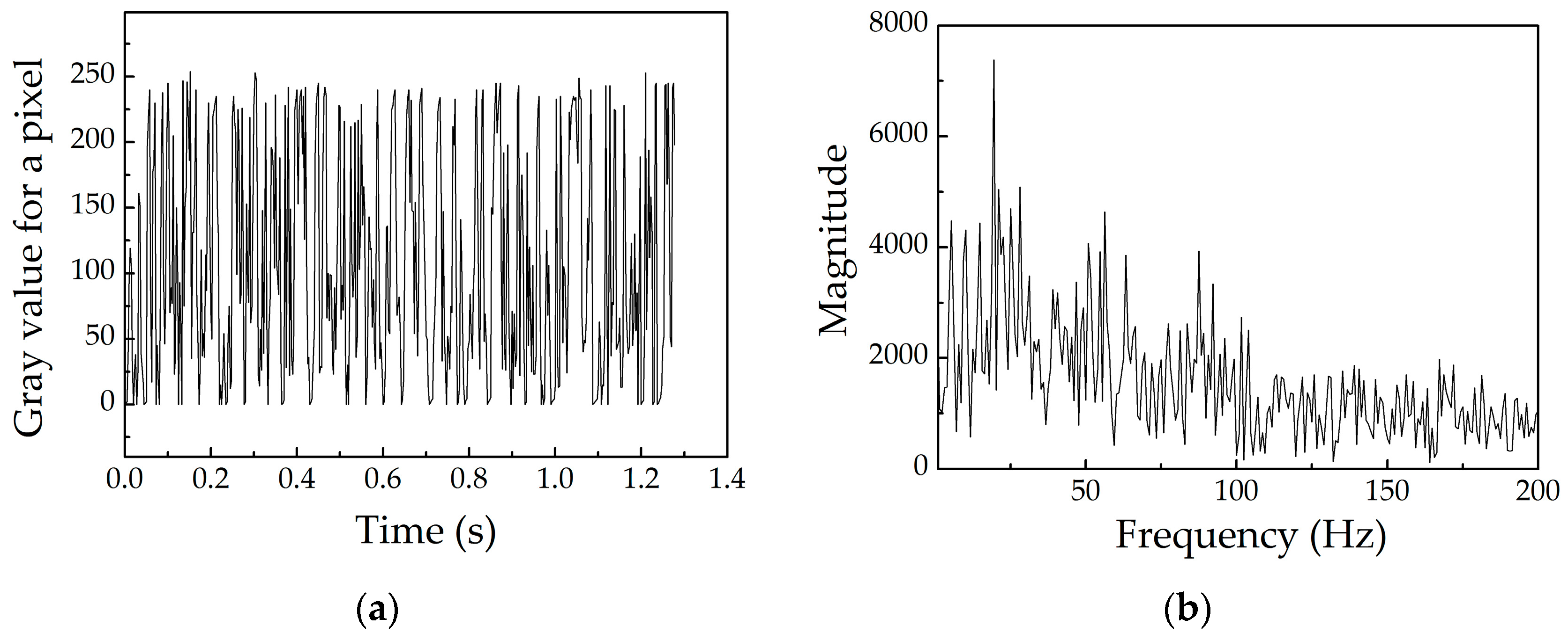
• Flickering weighted average frequency F [29,30]: the flickering spectrum contains multiple frequencies with large amplitudes, as will be displayed in the latter section. Therefore, a comprehensive parameter F is defined to consider the contributions of all components over the entire spectrum. It is a weighted average frequency and can be obtained by Equation (2).

  $$F=\frac{{\displaystyle \sum _{m=0}^{N-1}\left|X(f_m)\right|\cdot f_m}}{{\displaystyle \sum _{k=0}^{N-1}\left|X(f_m)\right|}}$$

  (2)

  where f_m is the mth frequency component, that is, f_m = mf_s/N; f_s is the image sampling rate (frame rate); and X(f_m) is the DFT (discrete Fourier transformation) calculating result of f_m, which is determined by Equation (3).

  $$X(f_m)={\displaystyle \sum _{i=1}^{N}l(t_i)\cdot \exp (}-j2\pi f_m{t}_i)$$

  (3)
• Flickering coefficient of variation c_v: the standard deviation σ is a well-known parameter to evaluate the variability or dispersion within a set of data. In general, a small σ indicates that the values approach the average, while a large σ implies that the data distribute over a large range of values. However, when the comparison is performed within different data groups, the use of σ has an assumption that their mean values are equal (or approximately equal). If the mean values of compared data sets have a significant difference, the σ is not suitable because it will bring large errors. To replace the position of σ under this situation, the coefficient of variation c_v is firstly introduced to estimate the oscillation amplitude. The c_v is a dimensionless parameter, which is defined as the normalized standard deviation, that is, the σ normalized by mean value, as shown in Equation (4). By employing c_v, the effects of diverse mean values can be eliminated. In present investigation, the flame mean luminosity varies considerably under varying mass flow rate of the fuel, and the distribution of mean gray value for a pixel also differs significantly, as exhibited in the latter section. Therefore, the coefficient of variation c_v is applied.

  $$c_v=\frac{\sigma }{l}=\frac{\sqrt{\frac{1}{N}{\displaystyle \sum _{i=1}^N{(l(t_i)-l)}^2}}}{l}$$

  (4)
• Skewness s: used to evaluate the asymmetry of the probability distribution of a data group around the mean value, which is defined by Equation (5). The s can be 0, positive, or negative. s = 0 indicates that the distribution is perfectly symmetric. s < 0 implies that the number of the values above the mean are larger than that below the mean, and the distribution is said to be left-skewed. On the contrary, s > 0 represents that the number of the values below the mean are larger than that above the mean, and the distribution is said to be right-skewed.

  $$s=\frac{\frac{1}{N}{\displaystyle \sum _{i=1}^N{(l(t_i)-l)}^3}}{{\sigma }^3}$$

  (5)
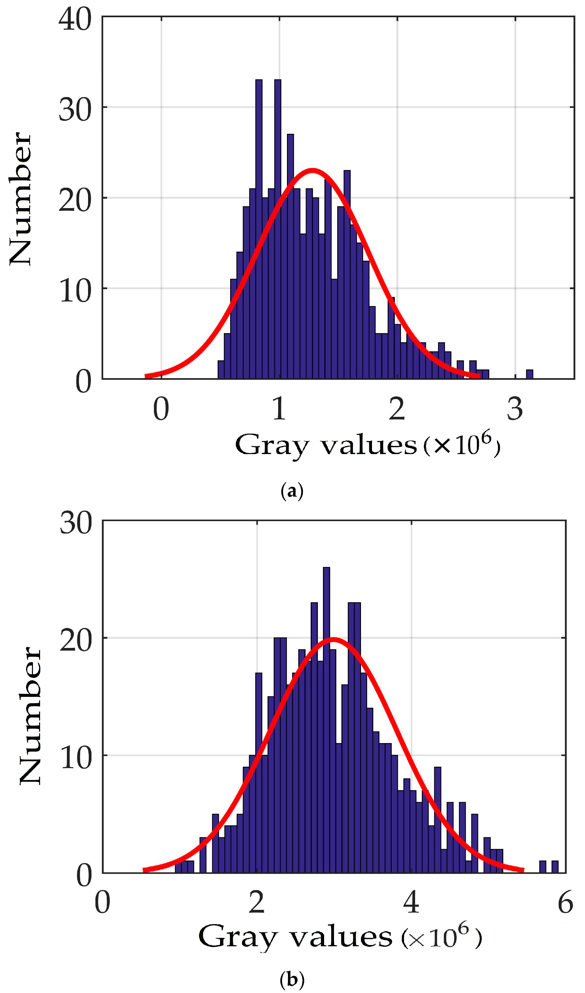
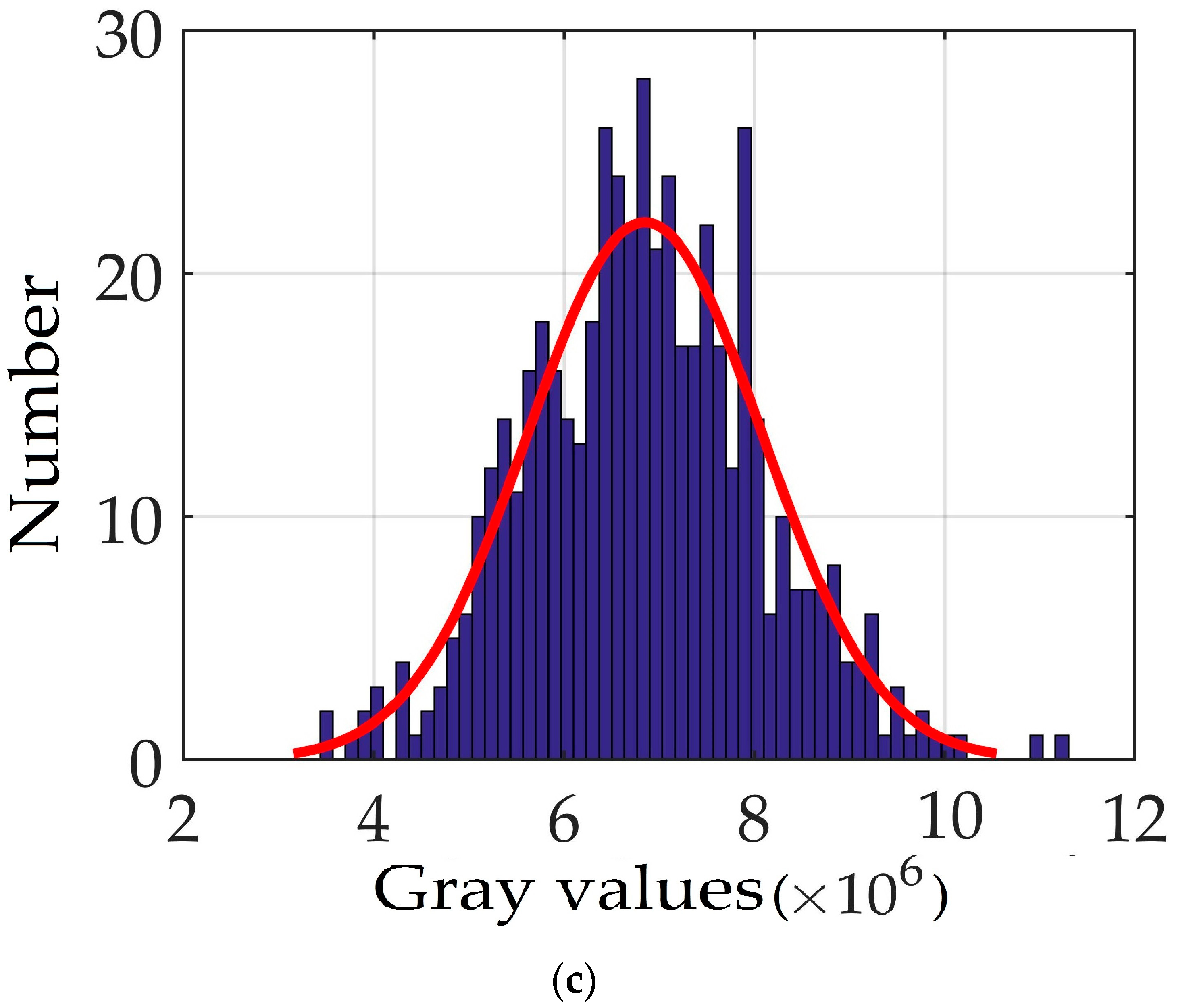
• Kurtosis k: used to describe the ‘peakedness’ of a distribution in comparison with its corresponding normal distribution, as defined by Equation (6). The value of k for normal distribution is 3, k > 3 indicates the shape of the distribution is sharper than normal distribution. A large value of k implies a strong peakedness in distribution values.

  $$s=\frac{\frac{1}{N}{\displaystyle \sum _{i=1}^N{(l(t_i)-l)}^4}}{{\sigma }^4}$$

  (6)

3.2. Analysis Methods

Two types of analysis methods were implemented to explore the local and overall information of flame flickering; they are presented as the following.

• Spatial analysis: for the same pixel in each image, the gray values registered by all pixels constitute a time luminance signal, with a length of N (i.e., the number of image series). For each operating condition, a total of x*y (as mentioned above) time signals are calculated for the oscillation parameters as defined before. The calculation result is an image, which reveals the spatial distribution of flame flickering.
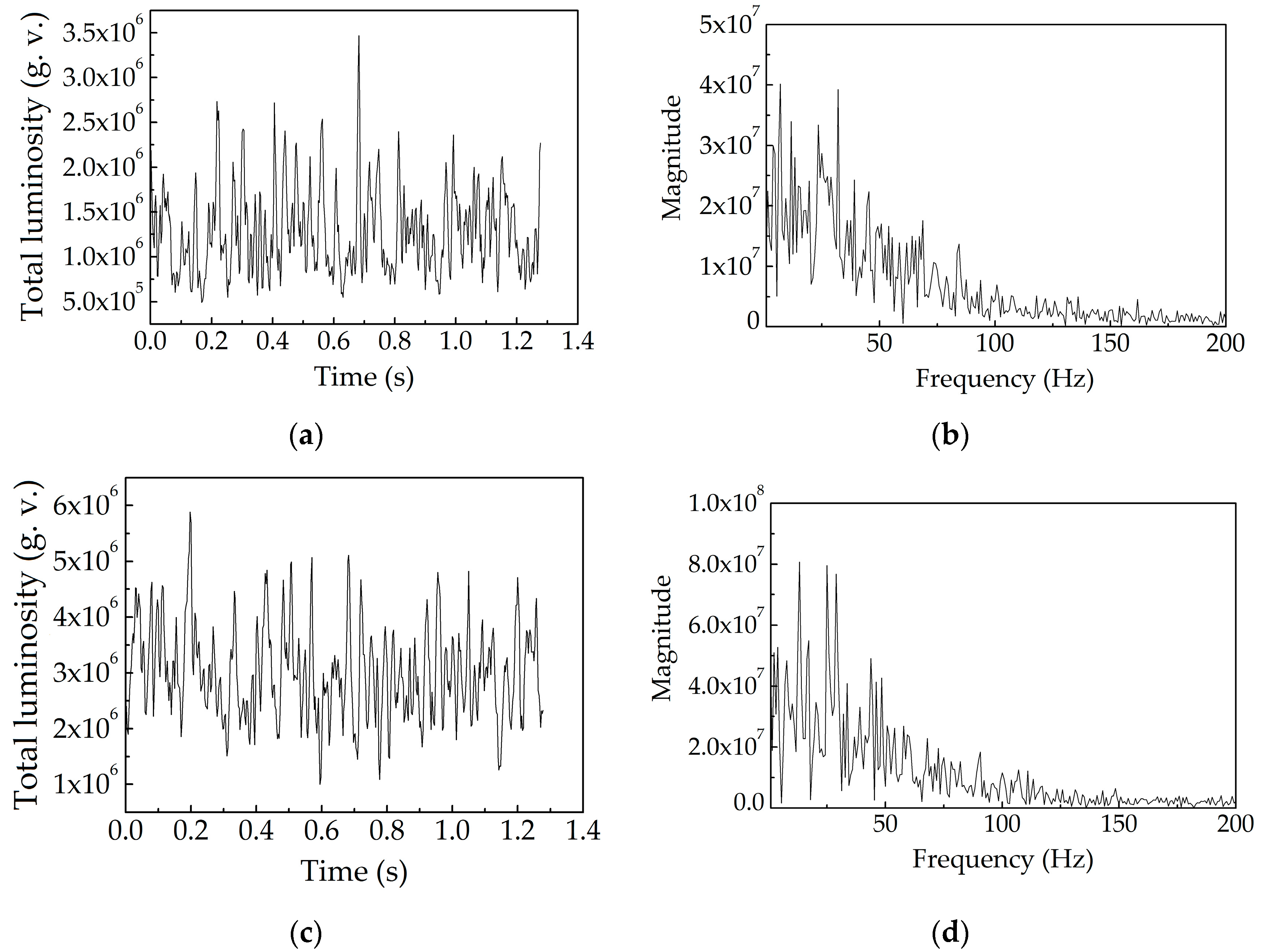
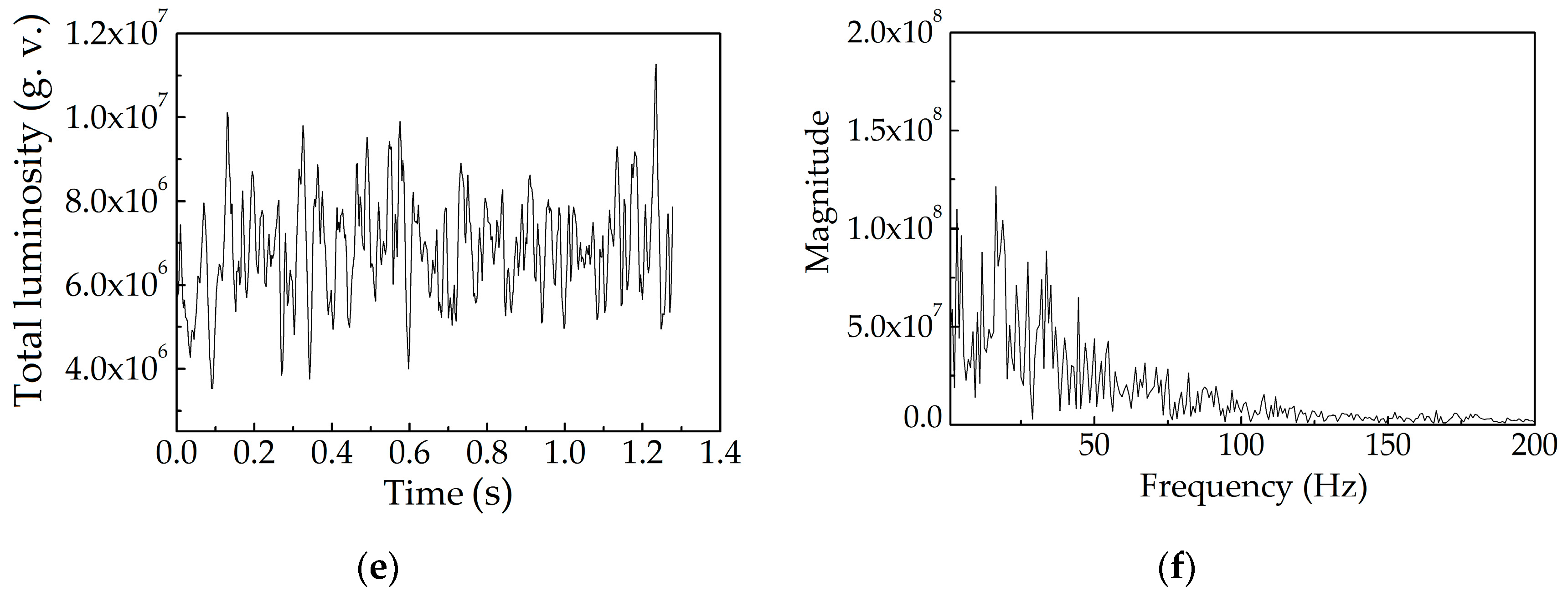
• Global analysis: for each image, the gray values all over an image are summed as a total luminosity, all total luminosities from a series of images make up a global time luminance signal for each case, which is processed to obtain global oscillation information.

In the present measurement setup, the frame rate of a video recorded with the high-speed camera was 400 fps (frame per second). The original resolution of a frame grabbed from the video was 1280 H × 1024 V pixels. To reduce the unnecessary calculation cost, its size was trimmed to 431 H × 601 V pixels. In each case, a sequence of continuous 512 images were employed to perform spatial analysis and global analysis, while the corresponding time length was 1.28 s.

4. Results and Discussion

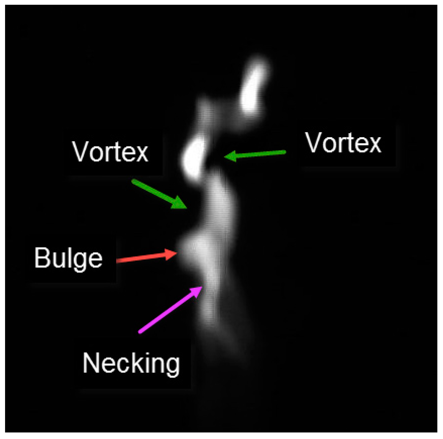
4.1. Flicker Shape

Flame flickering is a consequence of the flame-vortex interaction, as displayed in Figure 2. The vortices are generated outside the flame surface, because of the effect of buoyancy produced by the difference of density between hot combustion products and cool ambient air. These vortices move upward around flame front, forming a structure of bulge and necking. Old vortices shed from the flame tip, new vortices formed at the flame root and continue to travels along the flame surface, leading to the flame flickering. More details of flickering dynamics can be found in previous research [26].

4.2. Spatial Analysis

4.2.1. Flickering Signal for a Pixel

The time variation in gray value for a pixel (as an example) is shown in Figure 3a, and the corresponding magnitude–frequency curve (by the DFT) is presented in Figure 3b. It can be observed that multiple peak values exist in the spectrum, mainly concentrated on the range of 0–110 Hz, the components larger than 110 Hz were relatively small and can be negligible. Therefore, the frequency domain of 0–110 Hz was applied to calculate F according to Equation (2). For each case, a total of 601 × 431 signals (with a length of 512 for each signal) was processed to obtain the spatial distributions of the parameters.

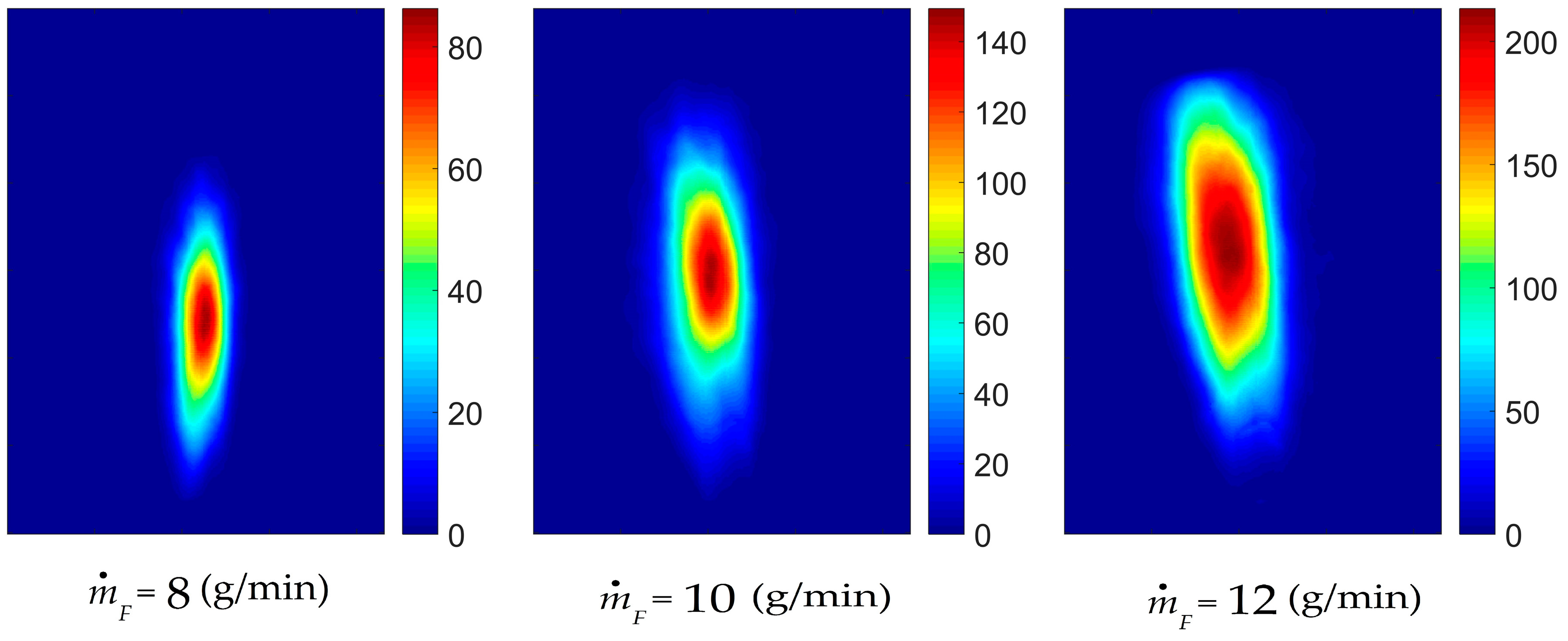
4.2.2. The Distribution of Mean Value

Figure 4 shows the influence of the mass flow rate of fuel $\dot{m}$_F on the averaged flame image. The mean flame appearance is comparatively regular, even though the flicker shape at each instant was irregular (as displayed in Figure 2). One can see that the distribution of flame averaged brightness for all cases is similar, that is, the brightest part is located in the core of flame zone, and the brightness gradually decreases from the inside out. With the increment of $\dot{m}$_F, the flame shape expanded because more air entrainment was required to burn the fuel. Moreover, the high levels of luminosity and its region were enhanced at larger $\dot{m}$_F, which indicated that the combustion intensity was increased as $\dot{m}$_F increased.

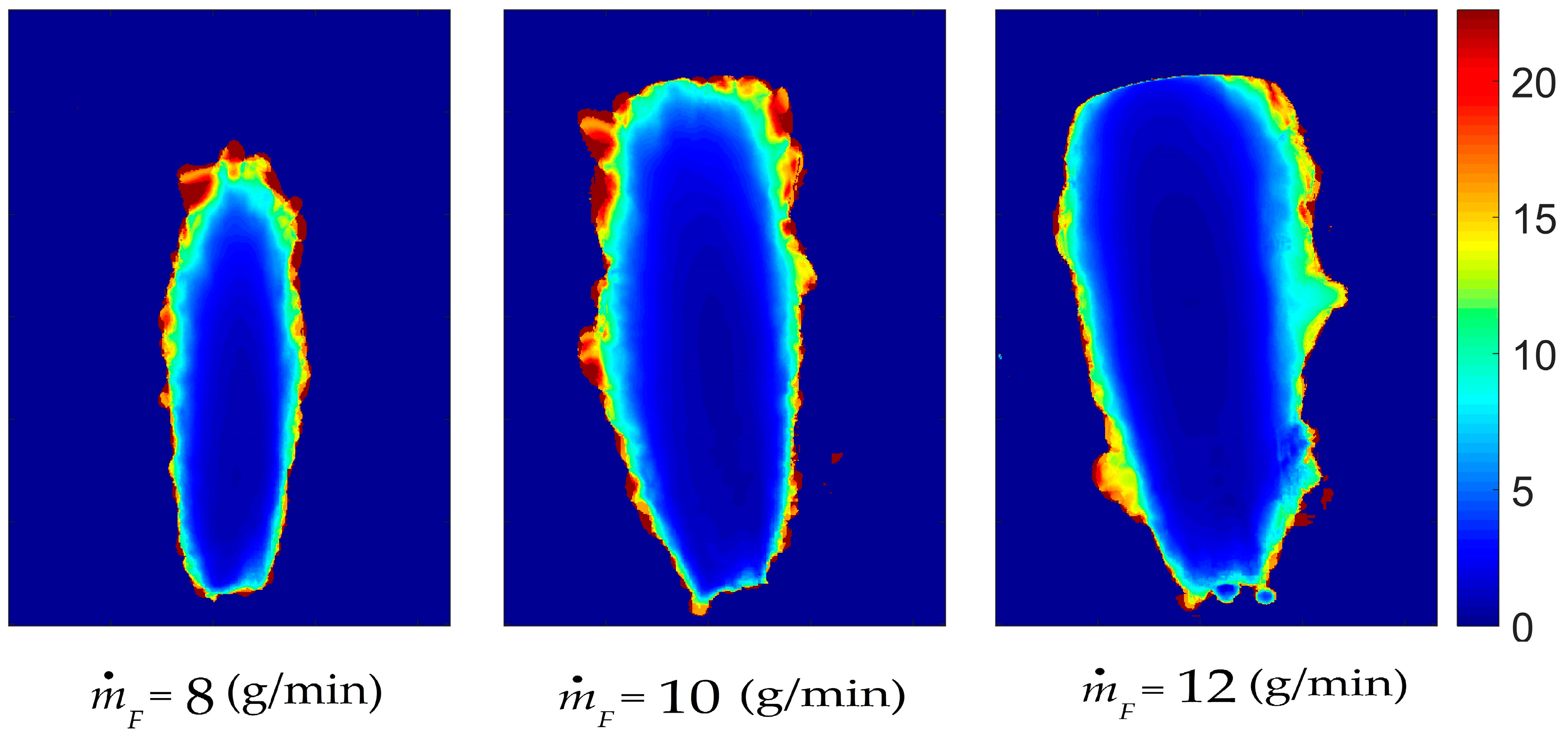
4.2.3. The Distribution of Flickering Weighted Average Frequency

Figure 5 displays the spatial arrangement of the flickering weighted average frequency F under varying mass flow rate of fuel. It can be found that, for all cases, the largest F mainly lay in the flickering edge, with a value of about 55 Hz. This means the velocity of pulsation at the edge is the fastest. This place corresponds to the position where minimal mean value existed, as can be seen in Figure 4. Meanwhile, the F diminished from the flicker outside in, the lowest F in all cases was close to 40 Hz, which was significantly observed inside the flickering under $\dot{m}$_F = 12 g/min. The distribution in interior zone was not continuous, and was composed of many discrete small regions with diverse values of F. Also, with the increment of $\dot{m}$_F, the distribution area enlarged as the flame zone became larger at higher $\dot{m}$_F. Altogether, the overall F all over the distribution declined as $\dot{m}$_F increased.

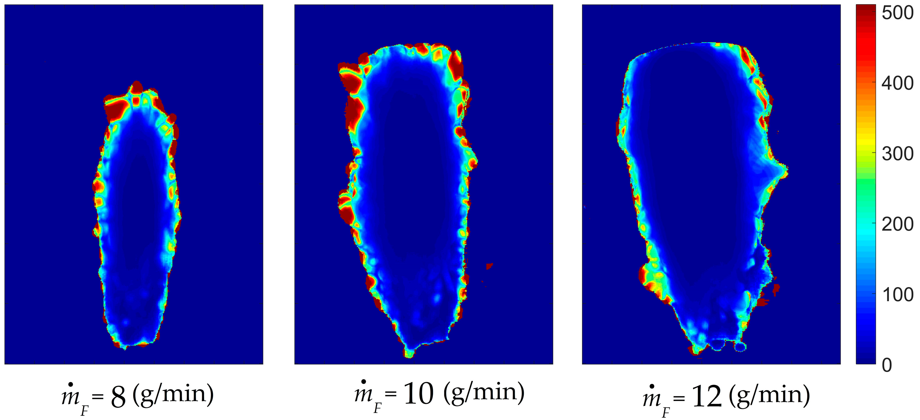
4.2.4. The Distribution of Flickering Coefficient of Variation

As the mean value for a pixel in Figure 4 was varying with pixel, the coefficient of variation c_v (i.e., normalized standard deviation by mean value) was thus (firstly) applied to measure the flickering oscillation amplitude, as introduced in the previous section. The calculation result of c_v under varying mass flow rate of fuel is exhibited in Figure 6. It can be noticed that, for all conditions, high levels of c_v (10–20) is positioned in the flickering edge, which is only a small region. From the edge outside in, the value of c_v sharply declines, most part of flickering inner region shows a low magnitude of c_v (0–5), with a smooth distribution. This is not coincident with the distribution of F at the same zone in Figure 5, which presented a scattered distribution as stated before. The distribution of c_v indicated that the strongest fluctuation occurs at the flickering border, while the inner zone is relatively stable. Moreover, for the flickering edge, as $\dot{m}$_F increased from 8 g/min to 10 g/min, the distribution shape seems basically unchanged; but as $\dot{m}$_F increased from 10 g/min to 12 g/min, the area where highest value of c_v is located (c_v ≥ 20, red color part in the Figure) reduced. This implied that the flickering has better stability at high mass flow rate of fuel.

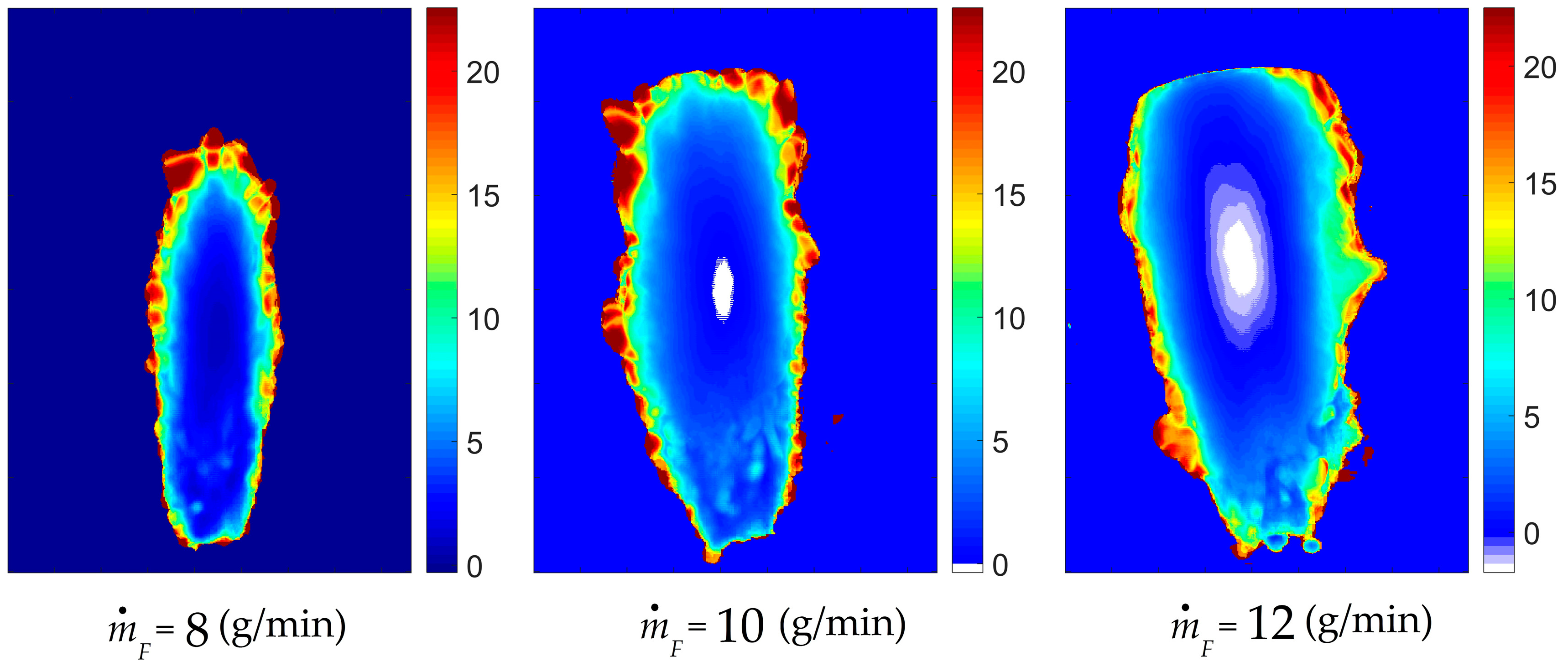
4.2.5. The Distribution of Skewness

With regard to skewness s, its calculation result is depicted in Figure 7. It can be observed that, for all conditions, the distribution of skewness at the flickering border is almost identical to that of the coefficient of variation in Figure 6, even the range of value is nearly the same. That is to say, the largest value of s also concentrated on flickering edge, which indicates the data sets at this small region are the most skewed. A large proportion of the flickering region had a positive value, which implies the major parts are right-skewed, that is, the values are concentrated below the mean. Meanwhile, there is a noticeable region in which the values of s are negative. The region was found in the core of the flickering zone under the cases when $\dot{m}$_F = 10 g/min and $\dot{m}$_F = 12 g/min, as presented by white color in the Figure 7. This negative-s region is left-skewed, that is, the values are concentrated above the mean. At the same time, it corresponds to the brightest parts in Figure 4. Moreover, no negative value of s was found for $\dot{m}$_F = 8 g/min. As $\dot{m}$_F increased from 8 g/min to 10 g/min, a small region with s < 0 appeared in the center of flickering; as $\dot{m}$_F increased from 10 g/min to 12 g/min, the region was expanded rapidly. This means that with the increasing of $\dot{m}$_F, the flickering region becomes increasingly more left-skewed.

4.2.6. The Distribution of Kurtosis

Concerning the kurtosis k, its spatial arrangement under varying mass flow rate of fuel is presented in Figure 8. One can observe that the distribution of kurtosis is accordant with that of the coefficient of variation in Figure 6 and the skewness in Figure 7 at the flickering edge. It is a thin layer through which a sharp change in k occurs (from 200 to 500), which indicates the data groups with large peakedness of probability distribution are situated in the flickering border. While the most flickering area has a low value of k (k < 100), where the probability distribution of data sets has a relatively small peakedness. When $\dot{m}$_F increased from 8 g/min to 10 g/min, the distribution shape remained unchanged appropriately; but when $\dot{m}$_F increased from 10 g/min to 12 g/min, the area where highest value of k locates (k ≥ 400, red color part in the Figure) diminished.

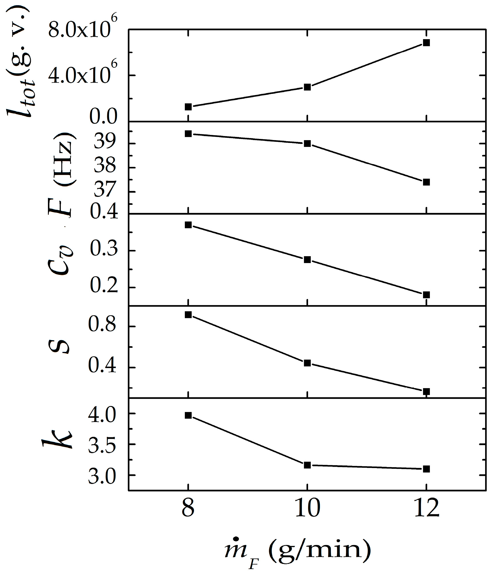
4.3. Global Analysis

To perform a global analysis, the gray values all over an image were summed as a total luminosity and thus generated one global time luminance signal for each case, as exhibited in Figure 9a,c,e—the corresponding spectrums (y the DFT) are presented in Figure 9b,d,f, respectively. The magnitude–frequency curve for all cases displays a multifrequency behavior. This may be attributed to the effects of swirl flow and partially premixing. The non-swirl flame always produces a single-peak spectrum [1,3]. Moreover, Huang et al. [29] found in their experimental results that the spectrum of a pure diffusion flame displays a single-peak behavior, but the spectrum of a premixed flame shows numerous peak values. Therefore, the swirl partially premixing could induce the multifrequency phenomenon. The frequency components for all cases are primarily concentrated in the range of 0–110 Hz (equal to that for a pixel), so other components were ignored while calculating the weighted average frequency F of global signals. The global signals were processed to obtain the global parameters; the calculation result is shown in Figure 10.

As illustrated in Figure 10, with the increase of $\dot{m}$_F, the mean luminosity of global signal l_tot intensified as the heat-release intensity increased. This is consistent with the observation from Figure 4. With regard to the global flickering weighted average frequency F, it slightly decreased from 39 Hz to 37 Hz as $\dot{m}$_F increased. Though this variation in F is not much (in the range of 2 Hz) yet, the spectrums as well as the dominant frequencies are entirely different. As we observed in previous research [26], the most dominant frequency increased with $\dot{m}$_F. However, the weighted average F in the present investigation did not follow this increasing trend because it was determined by all the selected components, therefore, its variation trend can be different from the most dominant frequency. Moreover, the values of global F are lower than that of local F from the distribution in Figure 5 (40–55 Hz).

Regarding the coefficient of variation c_v, it declined uniformly from 0.37 to 0.18 with the increment of $\dot{m}$_F, which means the oscillation amplitude diminished and thus the flame became more stable at larger $\dot{m}$_F. This agrees with the previous observation of normalized peak-to-peak amplitude [26], which also displayed a decreasing tendency with $\dot{m}$_F.

With respect to the skewness s and kurtosis k, the s linearly reduced as $\dot{m}$_F increased, and the k also had a decreasing trend with $\dot{m}$_F. The values of s for all cases are larger than 0, which means the number of the values below the mean are larger than that above the mean. Also, the values of k for all cases are larger than 3 (k is 3 for normal distribution), which implies the peakedness of number distributions are higher than the relevant normal distribution, as presented in Figure 11. The decreasing s indicates the number distribution becomes increasingly more symmetric, and the decreasing k indicates the number distribution becomes increasingly more flat. Both parameters jointly indicate that as $\dot{m}$_F increases, the number distribution progressively tends to normal distribution, that is, the normality of distribution improves, this can be easily observed in the Figure.

5. Conclusions

Based on an experiment, the flickering parameters under varying mass flow rate of fuel $\dot{m}$_F were investigated using two kinds of methods: spatial analysis and global analysis. The results can help in understanding flame oscillation in theory and can also be taken as reference in practical implementation. The primary conclusions of this work are summarized as follows:

• From the spatial analysis, the brightest part of flame was located in its core, and the brightness gradually decreased from the inside out. As $\dot{m}$_F increased, high levels of luminosity and its corresponding region were enhanced.
• The largest flickering weighted average frequency F mainly lay in the flickering edge, where the velocity of pulsation was the fastest. Meanwhile, F diminished from the flicker outside in, the distribution in interior zone was not continuous, which was composed of many discrete small regions with diverse values of F.
• The coefficient of variation c_v was firstly introduced to measure the flickering oscillation amplitude. High levels of c_v were also positioned in the flickering edge, where the strongest fluctuation occurs. From the edge outside in, the value of c_v sharply declined, and the most part of flickering inner region showed a low magnitude with a smooth distribution.
• Likewise, the largest value of skewness s concentrated on flickering border, where the datasets were the most skewed. Most of the flickering region has a positive value, which implies the major parts are right-skewed. While the negative-s region is also found in the core of the flickering zone, it is left-skewed and corresponds to the brightest parts. As $\dot{m}$_F became larger, the negative-s region was expanded rapidly, which means the flickering region becomes increasingly more left-skewed.
• The distribution of kurtosis k was in accordance with that of the c_v, the data groups with large peakedness of probability distribution were situated in the flickering border. While the most flickering area had a low value, where the probability distribution of data sets had a relatively small peakedness.
• From the global analysis, with the increment of $\dot{m}$_F, the global F slightly decreased while the global c_v declined uniformly, which means the oscillation amplitude diminished and thus the flame became more stable. The global s linearly reduced and the global k also had a decreasing trend. The decreasing global s indicates the number distribution gradually became symmetric, and the decreasing global k indicates the number distribution progressively became flat. Consequently, the number distribution progressively tends to normal distribution at larger $\dot{m}$_F.

References

1. Malalasekera, W.M.G.; Versteeg, H.K.; Gilchrist, K. A Review of Research and an Experimental Study on the Pulsation of Buoyant Diffusion Flames and Pool Fires. Fire Mater. 1996, 20, 261–271. [Google Scholar] [CrossRef]
2. Pan, K.L.; Li, C.C.; Juan, W.C.; Yang, J.T. Low-frequency oscillation of a non-premixed flame on a bluff-body burner. Combust. Sci. Technol. 2009, 181, 1217–1230. [Google Scholar] [CrossRef]
3. Sahu, K.B.; Kundu, A.; Ganguly, R.; Datta, A. Effects of fuel type and equivalence ratios on the flickering of triple flames. Combust. Flame 2009, 156, 484–493. [Google Scholar] [CrossRef]
4. Bahadori, M.Y.; Zhou, L.; Stocker, D.P.; Hegde, U. Functional Dependence of Flame Flicker on Gravitational Level. AIAA J. 2001, 39, 1404–1406. [Google Scholar] [CrossRef]
5. Durox, D.; Yuan, T.; Villermaux, E. The Effect of Buoyancy on Flickering in Diffusion Flames. Combust. Sci. Technol. 1997, 124, 277–294. [Google Scholar] [CrossRef]
6. Arai, M.; Sato, H.; Amagai, K. Gravity effects on stability and flickering motion of diffusion flames. Combust. Flame 1999, 118, 293–300. [Google Scholar] [CrossRef]
7. Hamins, A.; Yang, J.C.; Kashiwagi, T. An experimental investigation of the pulsation frequency of flames. Symp. Combust. 1992, 24, 1695–1702. [Google Scholar] [CrossRef]
8. Cetegen, B.M.; Kasper, K.D. Experiments on the oscillatory behavior of buoyant plumes of helium and helium-air mixtures. Phys. Fluids 1996, 8, 2974–2984. [Google Scholar] [CrossRef]
9. Pagni, P.J. Pool vortex shedding frequencies. Appl. Mech. Rev. 1990, 43, 160. [Google Scholar]
10. Bejan, A. Predicting the pool fire vortex shedding frequency. J. Heat Transf. 1991, 113, 261–263. [Google Scholar] [CrossRef]
11. Yilmaz, N.; Lucero, R.E.; Donaldson, A.B.; Gill, W. Flow characterization of diffusion flame oscillations using particle image velocimetry. Exp. Fluids 2009, 46, 737–746. [Google Scholar] [CrossRef]
12. Yilmaz, N.; Donaldson, A.B.; Lucero, R.E. Experimental study of diffusion flame oscillations and empirical correlations. Energy Convers. Manag. 2008, 49, 3287–3291. [Google Scholar] [CrossRef]
13. Tang, F.; Hu, L.; Wang, Q.; Ding, Z. Flame pulsation frequency of conduction-controlled rectangular hydrocarbon pool fires of different aspect ratios in a sub-atmospheric pressure. Int. J. Heat Mass Transf. 2014, 76, 447–451. [Google Scholar] [CrossRef]
14. Gotoda, H.; Kawaguchi, S.; Saso, Y. Experiments on dynamical motion of buoyancy-induced flame instability under different oxygen concentration in ambient gas. Exp. Therm. Fluid Sci. 2008, 32, 1759–1765. [Google Scholar] [CrossRef]
15. Fang, J.; Tu, R.; Guan, J.F.; Wang, J.J.; Zhang, Y.M. Influence of low air pressure on combustion characteristics and flame pulsation frequency of pool fires. Fuel 2011, 90, 2760–2766. [Google Scholar] [CrossRef]
16. Wang, Q.; Hu, L.; Tang, F.; Zhang, X.; Delichatsios, M. Characterization and comparison of flame fluctuation range of a turbulent buoyant jet diffusion flame under reduced- and normal pressure atmosphere. Proc. Eng. 2013, 62, 211–218. [Google Scholar] [CrossRef]
17. Tao, C.F.; Cai, X.; Wang, X. Experimental Determination of Atmospheric Pressures Effects on Flames from Small Scale Pool Fires. J. Fire Sci. 2013, 31, 387–394. [Google Scholar] [CrossRef]
18. Pretrel, H.; Audouin, L. Periodic puffing instabilities of buoyant large-scale pool fires in a confined compartment. J. Fire Sci. 2013, 31, 197–210. [Google Scholar] [CrossRef]
19. Chen, X.; Lu, S.; Wang, X.; Liew, K.M.; Li, C.; Zhang, J. Pulsation Behavior of Pool Fires in a Confined Compartment with a Horizontal Opening. Fire Technol. 2016, 52, 515–531. [Google Scholar] [CrossRef]
20. Chen, X.; Lu, S.X. On the Analysis of Flame Pulsation and Fire Induced Vent Flow Oscillatory Behaviors in Confined Enclosures with Horizontal Openings. Proc. Eng. 2018, 211, 104–112. [Google Scholar] [CrossRef]
21. Kostiuk, L.W.; Cheng, R.K. The coupling of conical wrinkled laminar flames with gravity. Combust. Flame 1995, 103, 27–40. [Google Scholar] [CrossRef]
22. Gotoda, H.; Maeda, K.; Ueda, T.; Cheng, R.K. Periodic motion of a Bunsen flame tip with burner rotation. Combust. Flame 2003, 134, 67–79. [Google Scholar] [CrossRef]
23. Durox, D.; Baillot, F.; Scouflaire, P.; Prud’homme, R. Some effects of gravity on the behaviour of premixed flames. Combust. Flame 1990, 82, 66–74. [Google Scholar] [CrossRef]
24. Fujisawa, N.; Abe, T.; Yamagata, T.; Tomidokoro, H. Flickering characteristics and temperature field of premixed methane/air flame under the influence of co-flow. Energy Convers. Manag. 2014, 78, 374–385. [Google Scholar] [CrossRef]
25. Bennett, B.A.V.; McEnally, C.S.; Pfefferle, L.D.; Smooke, M.D.; Colket, M.B. Computational and experimental study of axisymmetric coflow partially premixed ethylene/air flames. Combust. Flame 2001, 127, 2004–2022. [Google Scholar] [CrossRef]
26. Xi, Z.; Fu, Z.; Hu, X.; Sabir, S.W.; Jiang, Y. An Experimental Investigation on Flame Pulsation for a Swirl Non-Premixed Combustion. Energies 2018, 11, 1757. [Google Scholar] [CrossRef]
27. Samaniego, J.-M.; Egolfopoulos, F.N.; Bowman, C.T. CO2* Chemiluminescence in Premixed Flames. Combust. Sci. Technol. 1995, 109, 183–203. [Google Scholar] [CrossRef]
28. Li, M.; Tong, Y.; Klingmann, J.; Thern, M. Impact of vitiation on a swirl-stabilized and premixed methane flame. Energies 2017, 10, 1557. [Google Scholar] [CrossRef]
29. Huang, Y.; Yan, Y.; Lu, G.; Reed, A. On-line flicker measurement of gaseous flames by image processing and spectral analysis. Meas. Sci. Technol. 1999, 10, 726–733. [Google Scholar] [CrossRef]
30. González-Cencerrado, A.; Peña, B.; Gil, A. Coal flame characterization by means of digital image processing in a semi-industrial scale PF swirl burner. Appl. Energy 2012, 94, 375–384. [Google Scholar] [CrossRef]
Figure 1. The layout of the combustion device.
Energies 11 02430 g001
Figure 2. The appearance of flame flicker.
Energies 11 02430 g002
Figure 3. Time signal and spectrum for a pixel: (a) time trace and (b) spectrum curve.
Energies 11 02430 g003
Figure 4. The distribution of mean value for the mass flow rate of fuel.
Energies 11 02430 g004
Figure 5. The distribution of flickering weighted average frequency for the mass flow rate of fuel.
Energies 11 02430 g005
Figure 6. The distribution of coefficient of variation for the mass flow rate of fuel.
Energies 11 02430 g006
Figure 7. The distribution of skewness for the mass flow rate of fuel.
Energies 11 02430 g007
Figure 8. The distribution of kurtosis for the mass flow rate of fuel.
Energies 11 02430 g008
Figure 9. Time curve and corresponding spectrum of total luminosity for fuel mass flow rate: (a) time curve at m ˙ F = 8 g/min; (b) spectrum at m ˙ F = 8 g/min; (c) time curve at m ˙ F = 10 g/min; (d) spectrum at m ˙ F = 10 g/min; (e) time curve at m ˙ F = 12 g/min; (f) spectrum at m ˙ F = 12 g/min.
Energies 11 02430 g009aEnergies 11 02430 g009b
Figure 10. Flickering parameters of total luminosity for fuel mass flow rate.
Energies 11 02430 g010
Figure 11. The number distribution of total luminosity for fuel mass flow rate: (a) m ˙ F = 8 g/min; (b) m ˙ F = 10 g/min; (c) m ˙ F = 12 g/min.
Energies 11 02430 g011aEnergies 11 02430 g011b