Calculating Operational Patterns for Electric Vehicle Charging on a Real Distribution Network Based on Renewables’ Production

Abstract

The connection of electric vehicles to distribution networks has been an emerging issue of paramount importance for power systems. On one hand, it provides new opportunities for climate change mitigation, if electric energy used for charging is produced from zero emission sources. On the other hand, it stresses networks that are now required to accommodate, in addition to the loads and production from distributed generation they are initially designed for, loads from electric vehicles charging. In order to achieve maximum use of the grid without substantially affecting its performance, these issues have to be addressed in a coordinated manner, which requires adequate knowledge of the system under consideration. It is advantageous that electric vehicle charging can be controlled to a certain degree. This research provides better understanding of real distribution networks’ operation, proposing specific operational points through minimizing electric vehicle charging effects. The probabilistic Monte Carlo method on high performance computers is used for the calculations.

1. Introduction

A plethora of studies have been conducted to enhance understanding of electric vehicle connection to the grid [1], and to define expectations for electricity grid performance when distributed generation also plays its own important role [2,3]. These two, relatively new components require wise consideration [4] in order to enhance grids’ productivity; this has to be done in a manner which is interconnected [5]. One approach could be electric vehicles that are aggregated to a virtual power plant [6]; in conjunction to renewables generation, the degree to which they are able to increase grid capacity factors is investigated. Moreover, aggregation offers operational benefits to the system operator [7], who is then able to take faster and safer operational decisions. Electric vehicles batteries can present energy storage opportunities for the grid if customer comfort is lightly compromised. Under these conditions, it can provide short-term reserves and offer additional grid flexibility [8].

The increase of available computational power has also transferred to power system applications, thereby advancing the capability of researchers and operators to improve grid performance. This is a one-way path, due to the existing and increasing complexity of the addition of smart devices to the grid. Electric transportation is considered an important factor in this field [9]. Special attention is given to high performance computing (HPC) applications that use probabilistic methods, which are demanding in terms of calculations, but necessary to understand specific phenomena with adequate accuracy. Electric vehicle connections to the grid and the Monte Carlo method is an example [10]. However, stochastic methods, and especially Monte Carlo [11], is computationally demanding even for today’s standards; hence, specific operational points are developed in this study for a specific network [12].

Electric vehicles charging would also require a grid expansion design factor [13]. Current research on electric vehicles, as far as the distribution network is concerned, gives emphasis to probabilistic methods in order to predict charging patterns, and predict the expected charging behavior. This also affects the connection points for distributed generations, that could be optimally different if connected points are based on probabilistic methods, taking into consideration their intermittency [14]. As far as electric vehicles are concerned, the first step is to characterize their charging demand [15]. In some cases, the system is simulated as a whole, and the operational benefits are optimized based on electric charging owners’ behavior [16]. Alternatively, they are connected in a way that relieves distribution system constraints [17]. Active distribution network management could be done by aggregating electric vehicle behavior in a probabilistic manner [12]. Probabilistic studies have also shown good correlation between electric vehicles and renewables [18]. In this research, electric vehicle and load aggregation is performed on the level of a secondary distribution system, at the point of medium voltage (MV)/low voltage (LV) connection, and it is fully controlled.

Having mentioned the above, several studies have researched the emerging phenomenon of electric vehicles. All of them are consumer oriented, giving emphasis to electric vehicles per se, and showing minimal consideration for the electricity grid. On the other hand, the research presented in the current paper is electric grid oriented. It is focused in the procedure of creating optimal electric grid operation points for electric vehicle charging for a real distribution network [19], i.e., as it operates today, based on objective equations, solved with Monte Carlo using high performance computing.

2. Line under Investigation

This method is applied to a real representative distribution network [19]. Details of the network are available at the online dataset (http://dx.doi.org/10.7910/DVN/1I6MKU). Source code and data sets are open sourced to all users. This network spans fifty-five kilometers (55 km), a typical size for distribution rural lines, and its total installed load capacity is twelve mega-volt-amperes (12MVA). It is radially organized, and all conductors are optimized based on the expectation that higher currents appear near the feeder at the high to medium voltage substation.

It has forty-five (45) medium-to-low voltage transformers that are used to supply low voltage loads. These are the expected points for the aggregated connection of electric vehicles. The electric vehicles are connected to the secondary distribution network at low voltage levels, i.e., after the medium to low voltage transformers. It is assumed that the maximum load, including electric vehicles’, does not exceed the maximum observed active and reactive power of the existing installations. In this manner, the maximum utilization of the network is achieved.

Given that distribution network is limited, solar irradiation does not change significantly across the line. According to this assumption, production from photovoltaic plants could be safely assumed to be similar. Hence, the plants connected to the line under investigation would operate at the same percentage of installed capacity. There are also twenty-four (24) photovoltaic plants with an installed capacity totaling to 6929 ΜW. This network is not connected to any other type of distributed generation. The network in detail is available at [19].

3. Monte Carlo and Power Flow Methods

The Monte Carlo method is applied to numerically stochastic processes, and is used to simulate probabilistic physical phenomena. For this research, it is assumed that each of the forty-five (45) loading nodes of the line under consideration in this analysis can independently receive an active load Sn of up to 1 pu of its capacity:

$$0\le S_1\dots S_{45}\le 1 \mathrm{pu}$$

(1)

To achieve this input, a one-dimension table with 45 rows is defined that is assigned continuous random variables with values from 0 to 1. According to the following definition, a continuous random variable x has the properties of the function:

$${{\displaystyle \int }}_{-\infty }^{\infty }f\left(x\right)dx=F(\infty )=1$$

(2)

In other words, probability is uniform across all applicable values. However, in the reality of modern computing, absolute random numbers cannot be produced. Pseudorandom numbers are used, with satisfactory results. Pseudorandom number also demonstrate additional research related benefits. The same procedure has always been used to produce them, i.e., they are always the same for a given application. Therefore, results are replicable, hence better benchmarked and controlled.

AC power flow is the typical procedure for solving problems of power systems steady state analysis, which is also applied to this research [20]; it is a widely used and well-known procedure [21]. A typical element has the following admittance Yij:

$$Y_{ij}=\left|Y_{ij}\right|<{\Theta }_{ij}=\left|Y_{ij}\right|cos{\Theta }_{ij}+j\left|Y_{ij}\right|sin{\Theta }_{ij}=G_{ij}+j{B}_{ij}$$

(3)

and the voltage of a given bus is given as:

$$V_i=\left|V_i\right|<{\delta }_i=\left|V_i\right|cos{\delta }_i+j\left|V_i\right|sin{\delta }_i$$

(4)

the current of this bus is given from:

$$I_i=Y_{i1}{V}_1+Y_{i2}{V}_2+\dots +Y_{in}{V}_n={\displaystyle \sum }_{n=1}^N{Y}_{in}{V}_n$$

(5)

and its active and reactive power:

$$P_i+j{Q}_j=V_i^{*}{\displaystyle \sum }_{n=1}^N{Y}_{in}{V}_n$$

(6)

which makes:

$$P_i+j{Q}_j={\displaystyle \sum }_{n=1}^N\left|Y_{in}{V}_n{V}_i\right|<\left({\Theta }_{in}+{\delta }_n-{\delta }_i\right)$$

(7)

$$P_i={\displaystyle \sum }_{n=1}^N\left|Y_{in}{V}_n{V}_i\right|cos\left({\Theta }_{in}+{\delta }_n-{\delta }_i\right)$$

(8)

$$Q_i={\displaystyle \sum }_{n=1}^N\left|Y_{in}{V}_n{V}_i\right|sin\left({\Theta }_{in}+{\delta }_n-{\delta }_i\right)$$

(9)

at every time the scheduled power needs to be similar to the calculated:

$$\Delta P_i=P_{i,sch}-P_{i,calc}=\left(P_{gi}-P_{di}\right)-P_{i,calc}$$

(10)

$$\Delta Q_i=Q_{i,sch}-Q_{i,calc}=\left(Q_{gi}-Q_{di}\right)-Q_{i,calc}$$

(11)

and consequently

$$g_{i^{\prime }}=P_i-P_{i,sch}=P_i-\left(P_{gi}-P_{di}\right)=0$$

(12)

$$g_{i^{″}}=Q_i-Q_{i,sch}=Q_i-\left(Q_{gi}-Q_{di}\right)=0$$

(13)

the total active power loss is calculated by subtracting from the total generation the total load

$$P_L={\displaystyle \sum }_{i=1}^N{P}_i={\displaystyle \sum }_{i=1}^N{P}_{gi}-{\displaystyle \sum }_{i=1}^N{P}_{di}$$

(14)

and similarly, for the reactive power

$${\displaystyle \sum }_{i=1}^N{Q}_i={\displaystyle \sum }_{i=1}^N{Q}_{gi}-{\displaystyle \sum }_{i=1}^N{Q}_{di}$$

(15)

Newton-Raphson is the numerical method used to solve the above-mentioned equations. A short description is provided below. If two equations are considered:

$$g_1\left(x_1,x_2,u\right)=h_1\left(x_1,x_2,u\right)-b_1=0$$

(16)

$$g_2\left(x_1,x_2,u\right)=h_2\left(x_1,x_2,u\right)-b_2=0$$

(17)

then, the solutions $x_1^{*}$ and $x_2^{*}$ can be yielded from:

$$g_1\left(x_1^{*},x_2^{*},u\right)=g_1\left(x_1^{\left(0\right)}+\Delta x_1^{\left(0\right)},x_2^{\left(0\right)}+\Delta x_2^{\left(0\right)},u\right)=0$$

(18)

$$g_2\left(x_1^{*},x_2^{*},u\right)=g_2\left(x_1^{\left(0\right)}+\Delta x_1^{\left(0\right)},x_2^{\left(0\right)}+\Delta x_2^{\left(0\right)},u\right)=0$$

(19)

And then expanding in Taylor series:

$$g_1\left(x_1^{*},x_2^{*},u\right)=g_1\left(x_1^{\left(0\right)},x_2^{\left(0\right)},u\right)+\Delta x_1^{\left(0\right)}{\frac{\partial g_1}{\partial x_1}|}^0+\Delta x_2^{\left(0\right)}{\frac{\partial g_1}{\partial x_2}|}^0+\dots =0$$

(20)

$$g_2\left(x_1^{*},x_2^{*},u\right)=g_2\left(x_1^{\left(0\right)},x_2^{\left(0\right)},u\right)+\Delta x_1^{\left(0\right)}{\frac{\partial g_2}{\partial x_1}|}^0+\Delta x_2^{\left(0\right)}{\frac{\partial g_2}{\partial x_2}|}^0+\dots =0$$

(21)

which can be rewritten as:

$${\left[\begin{array}{cc}\frac{\partial g_1}{\partial x_1}& \frac{\partial g_1}{\partial x_2}\\ \frac{\partial g_2}{\partial x_1}& \frac{\partial g_2}{\partial x_2}\end{array}\right]}^{\left(0\right)}\left[\begin{array}{c}\Delta x_1^{\left(0\right)}\\ \Delta x_2^{\left(0\right)}\end{array}\right]=\left[\begin{array}{c}0-g_1\left(x_1^{\left(0\right)},x_2^{\left(0\right)},u\right)\\ 0-g_2\left(x_1^{\left(0\right)},x_2^{\left(0\right)},u\right)\end{array}\right] =\left[\begin{array}{c}{b}_1-h_1\left(x_1^{\left(0\right)},x_2^{\left(0\right)},u\right)\\ b_2-h_2\left(x_1^{\left(0\right)},x_2^{\left(0\right)},u\right)\end{array}\right]$$

(22)

where the Jacobian matrix is:

$$J^{\left(0\right)}={\left[\begin{array}{cc}\frac{\partial g_1}{\partial x_1}& \frac{\partial g_1}{\partial x_2}\\ \frac{\partial g_2}{\partial x_1}& \frac{\partial g_2}{\partial x_2}\end{array}\right]}^{\left(0\right)}$$

(23)

this gives:

$$J^{\left(0\right)}\left[\begin{array}{c}\Delta x_1^{\left(0\right)}\\ \Delta x_2^{\left(0\right)}\end{array}\right]=\left[\begin{array}{c}\Delta g_1^{\left(0\right)}\\ \Delta g_2^{\left(0\right)}\end{array}\right]$$

(24)

and the new estimates are:

$$x_1^{\left(1\right)}=x_1^{\left(0\right)}+\Delta x_1^{\left(0\right)}$$

(25)

$$x_2^{\left(1\right)}=x_2^{\left(0\right)}+\Delta x_2^{\left(0\right)}$$

(26)

4. Simulation Procedure

The source code for this publication has been simulated on Mathworks Matlab Runtime v92, 2017a [22], compiled on Unix operating system and run on Aris high performance computing [23]. High performance computing was not necessary to achieve the research goals; however, it reduces computational time and provides the capability of scaling up to larger electricity networks. Power load flow analysis is conducted on Matpower 6.0 code [24,25]. The source code and the results are provided in the supplementary materials of this manuscript, available on Harvard Dataverse [26].

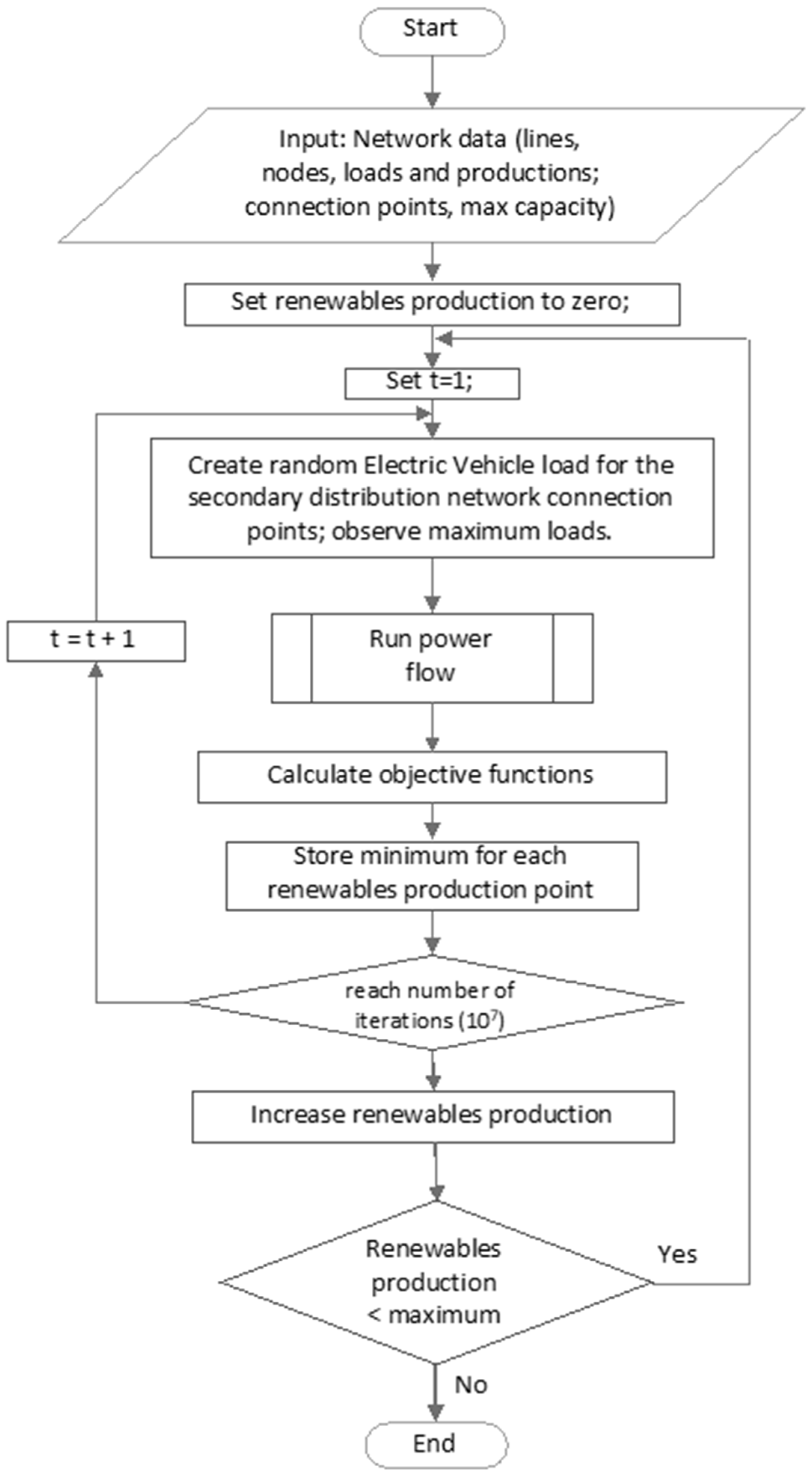
Figure 1 presents the flow chart for the proposed calculation method. Initially, the algorithm inputs the distribution network data. This includes information of its load and production nodes connection, line characteristics, as well as their impedance and reactance to perform load flow calculations. Then the system creates random loading using the Monte Carlo method [11] for all applicable nodes, and performs load flow analysis.

The procedure repeats numerous times in order to cover all applicable cases, and the best result is stored for each operational point. An ARIS high performance computer was able to simulate each one of the operational points, using one processor, in 48 h [23]. Source code total calculation time can be improved if the number of Monte Carlo iterations are reduced, but this could lead to suboptimal results. This source code may also run on personal computers, but usually higher computational times are required.

The default solver uses Newton’s method [20]. This type of analysis is adequate to perform load aggregation and production analysis in a steady state.

The objective functions applied to this research take into consideration the maximum electric vehicle charging load and the minimum voltage across the network, based on the available production from distributed generation. From these two aspects, the charging load is more important to the analysis, and consequently, it receives a higher contribution factor. The final objective is achieved by minimizing the following equations:

$$f_1\left(\mathrm{x}\right)=\underset{0\le \mathrm{x}\le 1}{\min }\left(0.5P_{EV}\left(\mathrm{x}\right)+0.5V_{min}\left(\mathrm{x}\right)\right)$$

(27)

$$f_2\left(\mathrm{x}\right)=\underset{0\le \mathrm{x}\le 1}{\min }\left(0.6P_{EV}\left(\mathrm{x}\right)+0.4V_{min}\left(\mathrm{x}\right)\right)$$

(28)

$$f_3\left(\mathrm{x}\right)=\underset{0\le \mathrm{x}\le 1}{\min }\left(0.7P_{EV}\left(\mathrm{x}\right)+0.3V_{min}\left(\mathrm{x}\right)\right)$$

(29)

$$f_4\left(\mathrm{x}\right)=\underset{0\le \mathrm{x}\le 1}{\min }\left(0.8P_{EV}\left(\mathrm{x}\right)+0.2V_{min}\left(\mathrm{x}\right)\right)$$

(30)

where:

Pev stands for the total active load of the line. It is assumed that $\cos \phi \approx 1$.

$$P_{ev}=\frac{{{\displaystyle \sum }}_1^{45}{S}_n}{S_{tot}},\mathrm{where}{S}_{tot}\mathrm{is}\mathrm{the}\mathrm{sum}\mathrm{of}\mathrm{all}\mathrm{loads}’\mathrm{installed}\mathrm{capacity}$$

(31)

and V_min is the minimum voltage observed at any node of the line.

All the above are calculated for increasing production from the connected-to-the-network distributed generation sources, such as photovoltaic plants. Then ten optimal operational points for each optimization equation were created, increasing renewables’ production from zero to maximum. These are operational points for a given network based on the availability of energy produced from renewables that meet the above-mentioned objective functions.

5. Results and Discussion

Simulation results have shown consistency across all applications to this work’s minimization formulas. According to the conducted simulations, there are repeating loading optimization patterns, unique for each line according to the imposed constraints in terms of distributed generation production and minimization requirements.

For $f_1\left(\mathrm{x}\right)$ there are five (5) operational points (

Table 1. Optimal loading per node according to $f_1\left(\mathrm{x}\right)$ for increasing production up to 50% of the distributed generator’s installed capacity.

#Transformer	${\mathit{f}}_1\left(\mathbf{x}\right)$-without DG (Percentage of Maximum Observed Load)	${\mathit{f}}_1\left(\mathbf{x}\right)$-10% DG (Percentage of Maximum Observed Load)	${\mathit{f}}_1\left(\mathbf{x}\right)$-20% DG (Percentage of Maximum Observed Load)	${\mathit{f}}_1\left(\mathbf{x}\right)$-30% DG (Percentage of Maximum Observed Load)	${\mathit{f}}_1\left(\mathbf{x}\right)$-40% DG (Percentage of Maximum Observed Load)	${\mathit{f}}_1\left(\mathbf{x}\right)$-50% DG (Percentage of Maximum Observed Load)
28	0.8382	0.0301	0.8382	0.8177	0.3908	0.152
31	0.8858	0.9023	0.8858	0.9598	0.9425	0.885
39	0.9049	0.9112	0.9049	0.8688	0.9894	0.9194
45	0.9762	0.925	0.9762	0.9796	0.9281	0.9924
49	0.3472	0.9478	0.3472	0.9235	0.9267	0.8259
61	0.6871	0.9702	0.6871	0.124	0.8382	0.478
74	0.8276	0.452	0.8276	0.7596	0.1854	0.9877
80	0.1646	0.6175	0.1646	0.3251	0.2775	0.3298
89	0.9733	0.8401	0.9733	0.8711	0.844	0.8278
91	0.5142	0.7913	0.5142	0.2599	0.8462	0.8417
92	0.6764	0.9131	0.6764	0.8997	0.8684	0.9708
39_18	0.9934	0.9186	0.9934	0.8458	0.7157	0.9316
39_51	0.9075	0.9167	0.9075	0.8253	0.9441	0.9404
39_51_3	0.8375	0.7877	0.8375	0.3792	0.2889	0.0673
39_94	0.8407	0.5423	0.8407	0.8235	0.9148	0.957
45_16A	0.8967	0.9474	0.8967	0.8395	0.314	0.6439
45_1A_4	0.2702	0.6134	0.2702	0.7997	0.8243	0.7673
49_9	0.7456	0.3974	0.7456	0.4233	0.2874	0.9802
61_10_6	0.3127	0.9037	0.3127	0.6078	0.9238	0.7111
61_28	0.5856	0.5735	0.5856	0.8873	0.7583	0.1116
61_28_9	0.8431	0.887	0.8431	0.3272	0.6855	0.9387
61_32_16	0.3256	0.8248	0.3256	0.6824	0.5453	0.0672
61_32_162	0.4562	0.4351	0.4562	0.5759	0.5438	0.5693
61_32_31	0.3894	0.0361	0.3894	0.8039	0.1964	0.6203
61_32_31_1	0.1494	0.1645	0.1494	0.0344	0.3047	0.533
61_45	0.0755	0.6439	0.0755	0.8028	0.9217	0.0153
61_45_12	0.8685	0.4486	0.8685	0.9713	0.4982	0.8222
61_45_4A_1	0.1951	0.3019	0.1951	0.7956	0.2272	0.879
61_5	0.6946	0.9572	0.6946	0.8117	0.619	0.9783
61_6_6A	0.7501	0.1219	0.7501	0.5161	0.2891	0.7149
61_7_2	0.7086	0.6227	0.7086	0.5581	0.7063	0.919
61_7_2_1A_2	0.3583	0.8671	0.3583	0.7513	0.4076	0.5091
61_7_2_2	0.2394	0.4019	0.2394	0.6523	0.716	0.4857
61_7_8	0.8612	0.9942	0.8612	0.8626	0.8057	0.9161
68_3	0.7148	0.807	0.7148	0.6459	0.2232	0.851
74_1A_4	0.7745	0.2404	0.7745	0.8569	0.8363	0.7064
74_1A_4_6	0.596	0.5571	0.596	0.1776	0.5202	0.4533
87_3	0.2453	0.3263	0.2453	0.1183	0.9159	0.8033
87_3_1	0.598	0.8487	0.598	0.12	0.8948	0.9351
92_21_4_3	0.1793	0.6066	0.1793	0.4977	0.1764	0.912
92_21_66	0.7871	0.5732	0.7871	0.7446	0.7469	0.1158
92_21A	0.3066	0.676	0.3066	0.8669	0.799	0.3738
92_30_1	0.201	0.5476	0.201	0.5093	0.033	0.8454
92_40	0.4673	0.3691	0.4673	0.1872	0.2473	0.1147
92_8_1	0.9249	0.0075	0.9249	0.247	0.4304	0.2284

and

Table 2. Optimal loading per node according to $f_1\left(\mathrm{x}\right)$, for increasing production from to 50% to full of the distributed generator’s installed capacity.

#Transformer	${\mathit{f}}_1\left(\mathbf{x}\right)$-60% DG, 70% DG, 80% DG, 90% DG and Full DG Production (Percentage of Maximum Observed Load)	#Transformer	${\mathit{f}}_1\left(\mathbf{x}\right)$-60% DG, 70% DG, 80% DG, 90% DG and Full DG Production (Percentage of Maximum Observed Load)	#Transformer	${\mathit{f}}_1\left(\mathbf{x}\right)$-60% DG, 70% DG, 80% DG, 90% DG and Full DG Production (Percentage of Maximum Observed Load)
28	0.152	45_16A	0.6439	61_7_2	0.919
31	0.885	45_1A_4	0.7673	61_7_2_1A_2	0.5091
39	0.9194	49_9	0.9802	61_7_2_2	0.4857
45	0.9924	61_10_6	0.7111	61_7_8	0.9161
49	0.8259	61_28	0.1116	68_3	0.851
61	0.478	61_28_9	0.9387	74_1A_4	0.7064
74	0.9877	61_32_16	0.0672	74_1A_4_6	0.4533
80	0.3298	61_32_162	0.5693	87_3	0.8033
89	0.8278	61_32_31	0.6203	87_3_1	0.9351
91	0.8417	61_32_31_1	0.533	92_21_4_3	0.912
92	0.9708	61_45	0.0153	92_21_66	0.1158
39_18	0.9316	61_45_12	0.8222	92_21A	0.3738
39_51	0.9404	61_45_4A_1	0.879	92_30_1	0.8454
39_51_3	0.0673	61_5	0.9783	92_40	0.1147
39_94	0.957	61_6_6A	0.7149	92_8_1	0.2284

) across the installed capacity of the distributed generation connected to the line. For each transformer connection node, the load percentage in conjunction to the maximum observed load has been calculated. It was observed that in some cases, this percentage is very low. This is due to the specific characteristics of the line, and hence, reinforcement is suggested near these transformers.

The exact manner in which this reinforcement shall be done is not currently clear to the researchers. A probabilistic approach can be applied, which can be part of future work. To achieve better performance, it is proposed that messed, instead of radial, topology be applied; however, issues of protection may arise.

For $f_2\left(\mathrm{x}\right)$, there are three (3) operational points (

Table 3. Optimal loading per node according to $f_2\left(\mathrm{x}\right)$ for increasing production up to 50% of the distributed generator’s installed capacity.

#Transformer	${\mathit{f}}_2\left(\mathbf{x}\right)$-without DG, 10% DG (Percentage of Maximum Observed Load)	${\mathit{f}}_2\left(\mathbf{x}\right)$-20% DG, 30% DG, 40% DG and 50% DG (Percentage of Maximum Observed Load)	#Transformer	${\mathit{f}}_2\left(\mathbf{x}\right)$-without DG, 10% DG (Percentage of Maximum Observed Load)	${\mathit{f}}_2\left(\mathbf{x}\right)$-20% DG, 30% DG, 40% DG and 50% DG (Percentage of Maximum Observed Load)
28	0.0301	0.152	61_32_31	0.0361	0.6203
31	0.9023	0.885	61_32_31_1	0.1645	0.533
39	0.9112	0.9194	61_45	0.6439	0.0153
45	0.925	0.9924	61_45_12	0.4486	0.8222
49	0.9478	0.8259	61_45_4A_1	0.3019	0.879
61	0.9702	0.478	61_5	0.9572	0.9783
74	0.452	0.9877	61_6_6A	0.1219	0.7149
80	0.6175	0.3298	61_7_2	0.6227	0.919
89	0.8401	0.8278	61_7_2_1A_2	0.8671	0.5091
91	0.7913	0.8417	61_7_2_2	0.4019	0.4857
92	0.9131	0.9708	61_7_8	0.9942	0.9161
39_18	0.9186	0.9316	68_3	0.807	0.851
39_51	0.9167	0.9404	74_1A_4	0.2404	0.7064
39_51_3	0.7877	0.0673	74_1A_4_6	0.5571	0.4533
39_94	0.5423	0.957	87_3	0.3263	0.8033
45_16A	0.9474	0.6439	87_3_1	0.8487	0.9351
45_1A_4	0.6134	0.7673	92_21_4_3	0.6066	0.912
49_9	0.3974	0.9802	92_21_66	0.5732	0.1158
61_10_6	0.9037	0.7111	92_21A	0.676	0.3738
61_28	0.5735	0.1116	92_30_1	0.5476	0.8454
61_28_9	0.887	0.9387	92_40	0.3691	0.1147
61_32_16	0.8248	0.0672	92_8_1	0.0075	0.2284
61_32_162	0.4351	0.5693

and

Table 4. Optimal loading per node according to $f_2\left(\mathrm{x}\right)$ for increasing production from to 50% to full of the distributed generator’s installed capacity.

#Transformer	${\mathit{f}}_2\left(\mathbf{x}\right)$-60% DG, 70% DG, 80% DG and 90% DG (Percentage of Maximum Observed Load)	${\mathit{f}}_2\left(\mathbf{x}\right)$-full DG Production (Percentage of Maximum Observed Load)	#Transformer	${\mathit{f}}_2\left(\mathbf{x}\right)$-60% DG, 70% DG, 80% DG and 90% DG (Percentage of Maximum Observed Load)	${\mathit{f}}_2\left(\mathbf{x}\right)$-Full DG Production (Percentage of Maximum Observed Load)
28	0.152	0.5311	61_32_31	0.6203	0.3476
31	0.885	0.9051	61_32_31_1	0.533	0.8526
39	0.9194	0.968	61_45	0.0153	0.881
45	0.9924	0.945	61_45_12	0.8222	0.5916
49	0.8259	0.6184	61_45_4A_1	0.879	0.7937
61	0.478	0.6175	61_5	0.9783	0.5695
74	0.9877	0.0504	61_6_6A	0.7149	0.5387
80	0.3298	0.9166	61_7_2	0.919	0.6669
89	0.8278	0.8561	61_7_2_1A_2	0.5091	0.765
91	0.8417	0.9359	61_7_2_2	0.4857	0.8833
92	0.9708	0.8999	61_7_8	0.9161	0.9672
39_18	0.9316	0.915	68_3	0.851	0.537
39_51	0.9404	0.9189	74_1A_4	0.7064	0.3431
39_51_3	0.0673	0.223	74_1A_4_6	0.4533	0.0839
39_94	0.957	0.7597	87_3	0.8033	0.4673
45_16A	0.6439	0.9474	87_3_1	0.9351	0.65
45_1A_4	0.7673	0.9928	92_21_4_3	0.912	0.4871
49_9	0.9802	0.9317	92_21_66	0.1158	0.8276
61_10_6	0.7111	0.5847	92_21A	0.3738	0.9753
61_28	0.1116	0.0368	92_30_1	0.8454	0.4514
61_28_9	0.9387	0.3133	92_40	0.1147	0.969
61_32_16	0.0672	0.1616	92_8_1	0.2284	0.7028
61_32_162	0.5693	0.7703

) across the installed capacity of the distributed generation connected to the line. To a certain degree, these are similar to the operational points derived from the other equations. This observation further supports the possibility of having line-specific optimal operation points across a wide range of operating conditions. This is to be further investigated.

For $f_3\left(\mathrm{x}\right)$, there are three (3) operational points (

Table 5. Optimal loading per node according to $f_3\left(\mathrm{x}\right)$ for increasing production up to the distributed generator’s installed capacity.

#Transformer	${\mathit{f}}_3\left(\mathbf{x}\right)$-without DG (Percentage of Maximum Observed Load)	${\mathit{f}}_3\left(\mathbf{x}\right)$-10% DG, 20% DG, 30% DG and 40% DG (Percentage of Maximum Observed Load)	${\mathit{f}}_3\left(\mathbf{x}\right)$-50% DG, 60% DG, 70% DG, 80% DG, 90% DG and Full DG Production (Percentage of Maximum Observed Load)
28	0.0301	0.152	0.5311
31	0.9023	0.885	0.9051
39	0.9112	0.9194	0.968
45	0.925	0.9924	0.945
49	0.9478	0.8259	0.6184
61	0.9702	0.478	0.6175
74	0.452	0.9877	0.0504
80	0.6175	0.3298	0.9166
89	0.8401	0.8278	0.8561
91	0.7913	0.8417	0.9359
92	0.9131	0.9708	0.8999
39_18	0.9186	0.9316	0.915
39_51	0.9167	0.9404	0.9189
39_51_3	0.7877	0.0673	0.223
39_94	0.5423	0.957	0.7597
45_16A	0.9474	0.6439	0.9474
45_1A_4	0.6134	0.7673	0.9928
49_9	0.3974	0.9802	0.9317
61_10_6	0.9037	0.7111	0.5847
61_28	0.5735	0.1116	0.0368
61_28_9	0.887	0.9387	0.3133
61_32_16	0.8248	0.0672	0.1616
61_32_162	0.4351	0.5693	0.7703
61_32_31	0.0361	0.6203	0.3476
61_32_31_1	0.1645	0.533	0.8526
61_45	0.6439	0.0153	0.881
61_45_12	0.4486	0.8222	0.5916
61_45_4A_1	0.3019	0.879	0.7937
61_5	0.9572	0.9783	0.5695
61_6_6A	0.1219	0.7149	0.5387
61_7_2	0.6227	0.919	0.6669
61_7_2_1A_2	0.8671	0.5091	0.765
61_7_2_2	0.4019	0.4857	0.8833
61_7_8	0.9942	0.9161	0.9672
68_3	0.807	0.851	0.537
74_1A_4	0.2404	0.7064	0.3431
74_1A_4_6	0.5571	0.4533	0.0839
87_3	0.3263	0.8033	0.4673
87_3_1	0.8487	0.9351	0.65
92_21_4_3	0.6066	0.912	0.4871
92_21_66	0.5732	0.1158	0.8276
92_21A	0.676	0.3738	0.9753
92_30_1	0.5476	0.8454	0.4514
92_40	0.3691	0.1147	0.969
92_8_1	0.0075	0.2284	0.7028

) across the installed capacity of the distributed generation connected to the line.

For $f_4\left(\mathrm{x}\right)$ there are two (2) operational points (

Table 6. Optimal loading per node according to $f_4\left(\mathrm{x}\right)$ for increasing production up to the distributed generator’s installed capacity.

#Transfomer	${\mathit{f}}_4\left(\mathbf{x}\right)$-without DG, 10% DG, 20% DG, 30% DG, 40% DG, 50% DG and 60% DG (Percentage of Maximum Observed Load)	${\mathit{f}}_4\left(\mathbf{x}\right)$-70% DG, 80% DG and 90% DG (Percentage of Maximum Observed Load)	${\mathit{f}}_4\left(\mathbf{x}\right)$-Full DG Production (Percentage of Maximum Observed Load)
28	0.5311	0.152	0.5311
31	0.9051	0.885	0.9051
39	0.968	0.9194	0.968
45	0.945	0.9924	0.945
49	0.6184	0.8259	0.6184
61	0.6175	0.478	0.6175
74	0.0504	0.9877	0.0504
80	0.9166	0.3298	0.9166
89	0.8561	0.8278	0.8561
91	0.9359	0.8417	0.9359
92	0.8999	0.9708	0.8999
39_18	0.915	0.9316	0.915
39_51	0.9189	0.9404	0.9189
39_51_3	0.223	0.0673	0.223
39_94	0.7597	0.957	0.7597
45_16A	0.9474	0.6439	0.9474
45_1A_4	0.9928	0.7673	0.9928
49_9	0.9317	0.9802	0.9317
61_10_6	0.5847	0.7111	0.5847
61_28	0.0368	0.1116	0.0368
61_28_9	0.3133	0.9387	0.3133
61_32_16	0.1616	0.0672	0.1616
61_32_162	0.7703	0.5693	0.7703
61_32_31	0.3476	0.6203	0.3476
61_32_31_1	0.8526	0.533	0.8526
61_45	0.881	0.0153	0.881
61_45_12	0.5916	0.8222	0.5916
61_45_4A_1	0.7937	0.879	0.7937
61_5	0.5695	0.9783	0.5695
61_6_6A	0.5387	0.7149	0.5387
61_7_2	0.6669	0.919	0.6669
61_7_2_1A_2	0.765	0.5091	0.765
61_7_2_2	0.8833	0.4857	0.8833
61_7_8	0.9672	0.9161	0.9672
68_3	0.537	0.851	0.537
74_1A_4	0.3431	0.7064	0.3431
74_1A_4_6	0.0839	0.4533	0.0839
87_3	0.4673	0.8033	0.4673
87_3_1	0.65	0.9351	0.65
92_21_4_3	0.4871	0.912	0.4871
92_21_66	0.8276	0.1158	0.8276
92_21A	0.9753	0.3738	0.9753
92_30_1	0.4514	0.8454	0.4514
92_40	0.969	0.1147	0.969
92_8_1	0.7028	0.2284	0.7028

) across the installed capacity of the distributed generation connected to the line.

It must be noted that, even if the equation results show an increasing value, the optimal line operation points remain, to a certain degree, of the same value. It appears that these are unique for each line, and can be pre-calculated. System operators, being able to affect electric vehicles’ load, can adjust grid’s operation near to these points. Grid reinforcements can be constructed on the objective of optimizing the optimization points, thereby achieving even better line performance when electric vehicles are to be connected. Moreover, in an effort to validate the obtained results, a genetic algorithm is applied in order to minimize the objective functions (25)–(28). Genetic algorithms are widely applied in science and engineering for solving practical search and optimization problems. The same algorithm gives excellent results in several other optimization problems [27,28,29]. The obtained results of the two applied methodologies (

Table 7. Minimization results for $f_1\left(\mathrm{x}\right)$ and $f_2$.

	Monte Carlo	GA		Monte Carlo	GA
$f_1\left(\mathrm{x}\right)$-without DG	0.7683	0.7944	$f_2\left(\mathrm{x}\right)$-without DG	0.7598	0.7865
$f_1\left(\mathrm{x}\right)$-10% DG	0.7872	0.7942	$f_2\left(\mathrm{x}\right)$-10% DG	0.7756	0.7857
$f_1\left(\mathrm{x}\right)$-20% DG	0.7997	0.7958	$f_2\left(\mathrm{x}\right)$-20% DG	0.7873	0.7926
$f_1\left(\mathrm{x}\right)$-30% DG	0.8097	0.7997	$f_2\left(\mathrm{x}\right)$-30% DG	0.7981	0.7918
$f_1\left(\mathrm{x}\right)$-40% DG	0.8175	0.8265	$f_2\left(\mathrm{x}\right)$-40% DG	0.8073	0.8117
$f_1\left(\mathrm{x}\right)$-50% DG	0.8261	0.8346	$f_2\left(\mathrm{x}\right)$-50% DG	0.8155	0.8316
$f_1\left(\mathrm{x}\right)$-60% DG	0.8351	0.8487	$f_2\left(\mathrm{x}\right)$-60% DG	0.8226	0.8500
$f_1\left(\mathrm{x}\right)$-70% DG	0.843	0.8346	$f_2\left(\mathrm{x}\right)$-70% DG	0.829	0.8328
$f_1\left(\mathrm{x}\right)$-80% DG	0.8499	0.8425	$f_2\left(\mathrm{x}\right)$-80% DG	0.8345	0.8329
$f_1\left(\mathrm{x}\right)$-90% DG	0.8521	0.8523	$f_2\left(\mathrm{x}\right)$-90% DG	0.8362	0.8439
$f_1\left(\mathrm{x}\right)$-full DG production	0.8537	0.8748	$f_2\left(\mathrm{x}\right)$-full DG production	0.8398	0.8728

and

Table 8. Minimization results for $f_3\left(\mathrm{x}\right)$ and $f_4\left(\mathrm{x}\right)$.

	Monte Carlo	GA		Monte Carlo	GA
$f_3\left(\mathrm{x}\right)$-without DG	0.7598	0.7821	$f_4\left(\mathrm{x}\right)$-without DG	0.7694	0.7694
$f_3\left(\mathrm{x}\right)$-10% DG	0.7741	0.7787	$f_4\left(\mathrm{x}\right)$-10% DG	0.7786	0.7786
$f_3\left(\mathrm{x}\right)$-20% DG	0.7837	0.7805	$f_4\left(\mathrm{x}\right)$-20% DG	0.7858	0.7858
$f_3\left(\mathrm{x}\right)$-30% DG	0.7918	0.7799	$f_4\left(\mathrm{x}\right)$-30% DG	0.7918	0.7918
$f_3\left(\mathrm{x}\right)$-40% DG	0.7987	0.8012	$f_4\left(\mathrm{x}\right)$-40% DG	0.7969	0.7969
$f_3\left(\mathrm{x}\right)$-50% DG	0.8053	0.8133	$f_4\left(\mathrm{x}\right)$-50% DG	0.8014	0.8014
$f_3\left(\mathrm{x}\right)$-60% DG	0.8111	0.8271	$f_4\left(\mathrm{x}\right)$-60% DG	0.8052	0.8052
$f_3\left(\mathrm{x}\right)$-70% DG	0.8162	0.8099	$f_4\left(\mathrm{x}\right)$-70% DG	0.829	0.829
$f_3\left(\mathrm{x}\right)$-80% DG	0.8207	0.8123	$f_4\left(\mathrm{x}\right)$-80% DG	0.8345	0.8345
$f_3\left(\mathrm{x}\right)$-90% DG	0.8247	0.8245	$f_4\left(\mathrm{x}\right)$-90% DG	0.8362	0.8362
$f_3\left(\mathrm{x}\right)$-full DG production	0.8282	0.8505	$f_4\left(\mathrm{x}\right)$-full DG production	0.8166	0.8166

) present adequate convergence, confirming the appropriateness of the proposed methodology.

6. Conclusions

This analysis provides specific operational points based on the production of the connected distributed generators. Based on these findings, potential charging service providers are able to optimize the charging of electric vehicles connected to the line under investigation. In this way, optimal operations could be achieved. It should be mentioned that it is possible to provide optimization formulas for minimizing line losses or maximizing transferred energy using the provided algorithm.

Loading patterns appear to be consistent across all performed calculations. It is believed that they are connected to the topology of the line, and are to a certain degree unconnected to the load. This is an important observation that requires further investigation.

It is observed that several transformer connection nodes display low percentages of optimal load. To the authors’ understanding, these are the areas of the grid that need reinforcement. The reinforcement can be done in a manner for the grid whereby the radial configuration is lost. In this case, new calculations are required.

Simulation results have shown improving performance of the grid for increasing production from distributed generators. This is an expected observation; however, the performed simulations are able to provide quantification.

Future work will include the creation of active protection systems based on pragmatic conditions operational system diagnosis, and further probabilistic analysis for possible reinforcements.

References

1. Morais, H.; Sousa, T.; Vale, Z.; Faria, P. Evaluation of the electric vehicle impact in the power demand curve in a smart grid environment. Energy Convers. Manag. 2014, 82, 268–282. [Google Scholar] [CrossRef] [Green Version]
2. Fang, X.; Misra, S.; Xue, G.; Yang, D. Smart Grid—The new and improved power grid: A survey. IEEE Commun. Surv. Tutor. 2012, 14, 944–980. [Google Scholar] [CrossRef]
3. Vita, V.; Alimardan, T.; Ekonomou, L. The impact of distributed generation in the distribution networks’ voltage profile and energy losses. In Proceedings of the 9th IEEE European Modelling Symposium on Mathematical Modelling and Computer Simulation, Madrid, Spain, 6–8 October 2015; pp. 260–265. [Google Scholar]
4. Rahbari, O.; Vafaeipour, M.; Omar, N.; Rosen, M.A.; Hegazy, O.; Timmermans, J.-M.; Heibati, S.; Bossche, P.V.D. An optimal versatile control approach for plug-in electric vehicles to integrate renewable energy sources and smart grids. Energy 2017, 134, 1053–1067. [Google Scholar] [CrossRef]
5. Farid, A.; Jiang, B.; Muzhikyan, A.; Youcef-Toumi, K. The need for holistic enterprise control assessment methods for the future electricity grid. Renew. Sustain. Energy Rev. 2016, 56, 669–685. [Google Scholar] [CrossRef]
6. Zakariazadeh, A.; Jadid, S.; Siano, P. Integrated operation of electric vehicles and renewable generation in a smart distribution system. Energy Convers. Manag. 2015, 89, 99–110. [Google Scholar] [CrossRef]
7. Bhattarai, B.P.; Myers, K.S.; Bak-Jensen, B.; Mendaza, I.D.d.C.; Turk, R.J.; Gentle, J.P. Optimum aggregation of geographically distributed flexible resources in strategic smart-grid/microgrid locations. Electr. Power Energy Syst. 2017, 92, 193–201. [Google Scholar] [CrossRef]
8. Knezovic, K.; Marinelli, M.; Zecchino, A.; Andersen, P.B.; Traeholt, C. Supporting involvement of electric vehicles in distribution grids: Lowering the barriers for a proactive integration. Energy 2017, 134, 458–468. [Google Scholar] [CrossRef]
9. Green, R.C.; Wang, L.; Alam, M. Applications and Trends of High Performance Computing for Electric Power Systems: Focusing on Smart Grid. IEEE Trans. Smart Grid 2013, 4, 422–431. [Google Scholar] [CrossRef]
10. Procopiou, A.T.; Quirós-Tortós, J.; Ochoa, L.F. HPC-Based Probabilistic Analysis of LV Networks with EVs: Impacts and Control. IEEE Trans. Smart Grid. 2017, 8, 1479–1487. [Google Scholar] [CrossRef]
11. Kalos, M.H.; Whitlock, P.A. Monte Carlo Methods; WILEY-VCH Verlag: Hoboken, NJ, USA, 2008. [Google Scholar]
12. Xiang, Y.; Liua, J.; Liu, Y. Optimal active distribution system management considering aggregated plug-in electric vehicles. Electr. Power Syst. Res. 2016, 131, 105–115. [Google Scholar] [CrossRef]
13. Abdelsamad, S.; Morsi, W.; Sidhu, T. Optimal secondary distribution system design considering plug-inelectric vehicles. Electr. Power Syst. Res. 2016, 130, 266–276. [Google Scholar] [CrossRef]
14. Sadeghi, M.; Kalantar, M. Multi types DG expansion dynamic planning in distribution system under stochastic conditions using Covariance Matrix Adaptation Evolutionary Strategy and Monte-Carlo simulation. Energy Convers. Manag. 2014, 87, 455–471. [Google Scholar] [CrossRef]
15. Sun, S.; Yang, Q.; Yan, W. A novel Markov-based temporal-SoC analysis for characterizing PEV charging demand. IEEE Trans. Ind. Inform. 2018, 14, 156–166. [Google Scholar] [CrossRef]
16. Arias, A.; Granada, M.; Castro, C.A. Optimal probabilistic charging of electric vehicles in distribution systems. IET Electr. Syst. Transp. 2017, 7, 246–251. [Google Scholar] [CrossRef]
17. Wu, F.; Sioshansi, R. A two-stage stochastic optimization model for scheduling electric vehicle charging loads to relieve distribution-system constraints. Transp. Res. Part B 2017, 102, 55–82. [Google Scholar] [CrossRef]
18. Wang, L.; Sharkh, S.; Chipperfield, A. Optimal decentralized coordination of electric vehicles and renewable generators in a distribution network using A* search. Electr. Power Energy Syst. 2018, 98, 474–487. [Google Scholar] [CrossRef]
19. Lazarou, S.; Vita, V.; Ekonomou, L. An open data repository for steady state analysis of a 100-node electricity distribution network with moderate connection of renewable energy sources. Data Brief 2018, 16, 1095–1101. [Google Scholar] [CrossRef] [PubMed]
20. Zimmerman, R.D.; Murillo-Sanchez, C.E. Matpower 6.0 User’s Manual; PSERC: Tempe, AZ, USA, 2016; Available online: http://www.pserc.cornell.edu/matpower/manual.pdf (accessed on 10 September 2018).
21. Grainger, J.J.; Stevenson, W.D. Power System Analysis; McGraw-Hill: New York, NY, USA, 1993. [Google Scholar]
22. Mathworks. Matlab Runtime. Available online: https://www.mathworks.com/products/compiler/matlab-runtime.html (accessed on 10 September 2018).
23. Greek Research and Technology Network (GRNET). Aris High Performance Computing. Available online: https://hpc.grnet.gr/ (accessed on 10 September 2018).
24. Zimmerman, R.D.; Murillo-Sánchez, C.E.; Thomas, R.J. MATPOWER: Steady-State Operations, Planning and Analysis Tools for Power Systems Research and Education. IEEE Trans. Power Syst. 2011, 26, 12–19. [Google Scholar] [CrossRef]
25. Murillo-Sánchez, C.E.; Zimmerman, R.D.; Anderson, C.L.; Thomas, R.J. Secure Planning and Operations of Systems with Stochastic Sources, Energy Storage and Active Demand. IEEE Trans. Smart Grid 2013, 4, 2220–2229. [Google Scholar] [CrossRef]
26. Lazarou, S.; Vita, V.; Christodoulou, C.; Ekonomou, L. Replication Data for: Calculating Operational Patterns for Electric Vehicle Charging on a Real Distribution Network Based on Renewables’ Production. Available online: http://dx.doi.org/10.7910/DVN/1MWESP (accessed on 10 September 2018).
27. Gonos, I.; Stathopulos, I. Estimation of multi-layer soil parameters using genetic algorithms. IEEE Trans. Power Deliv. 2005, 20, 100–106. [Google Scholar] [CrossRef]
28. Christodoulou, C.; Gonos, I.; Stathopulos, I. Estimation of the parameters of metal oxide gapless surge arrester equivalent circuit models using genetic algorithm. Electr. Power Syst. Res. 2011, 81, 1881–1886. [Google Scholar] [CrossRef]
29. Christodoulou, C.A.; Papanikolaou, N.P.; Gonos, I.F. Design of three-phase autonomous PV residential systems with improved power quality. IEEE Trans. Sustain. Energy 2014, 5, 1027–1035. [Google Scholar] [CrossRef]
Figure 1. Calculating operational points optimization formula minimums.
Energies 11 02400 g001