RANS and Hybrid RANS-LES Simulations of an H-Type Darrieus Vertical Axis Water Turbine

Abstract

Nowadays, the global energy crisis has encouraged the use of alternative sources like the energy available in the water currents of seas and rivers. The vertical axis water turbine (VAWT) is an interesting option to harness this energy due to its advantages of facile installation, maintenance and operation. However, it is known that its efficiency is lower than that of other types of turbines due to the unsteady effects present in its flow physics. This work aims to analyse through Computational Fluid Dynamics (CFD) the turbulent flow dynamics around a small scale VAWT confined in a hydrodynamic tunnel. The simulations were developed using the Unsteady Reynolds Averaged Navier Stokes (URANS), Detached Eddy Simulation (DES) and Delayed Detached Eddy Simulation (DDES) turbulence models, all of them based on k-ω Shear Stress Transport (SST). The results and analysis of the simulations are presented, illustrating the influence of the tip speed ratio. The numerical results of the URANS model show a similar behaviour with respect to the experimental power curve of the turbine using a lower number of elements than those used in the DES and DDES models. Finally, with the help of both the Q-criterion and field contours it is observed that the refinements made in the mesh adaptation process for the DES and DDES models improve the identification of the scales of the vorticity structures and the flow phenomena present on the near and far wake of the turbine.

1. Introduction

The high energy demand, the political instability of major oil-producing regions, the depletion of fossil fuel reserves and the environmental problems due to the continuing deterioration of the global ecosystems have raised concerns about the future of energy. With this perspective, renewable energies have come to play an important role in society in order to reduce or eradicate these problems.

Hydropower is one of the most important renewable energy sources and has a great development potential. While the technology of conventional hydropower plants using dams is mature, there are future opportunities to install small-scale facilities in small rivers and streams, water and sewage treatment plants, as well as industrial water channels and in this way take advantage of these water bodies and extract the energy for local consumption. To transform the kinetic energy stored in the rivers and seas tidal currents into electrical energy, turbines are used, and these can be classified into two types, horizontal and vertical axis turbines. Darrieus turbines with straight blades, also known as Type H turbines or Giromills, are the simplest and most popular among vertical axis turbines. The main advantages of this type of turbine, unlike horizontal axis turbines, is that these no need for a mechanism to orient their blades with regard to the fluid, so they can be located in places where there is a high variation in the direction of the current, and they are easy to build, install and maintain at lower costs thanks to their geometric simplicity [1]. Despite the large number of advantages that vertical axis turbines have, the useful energy that can be obtained from them is lower compared to horizontal axis ones [2]. This fact is due to a great variety of phenomena present in the flow dynamics, like the detachment of tip vortices, their interaction with the blades and the drag effect on the arms.

With the advances in high-performance computing in recent years, in terms of increasing the capabilities of computers and the development of more advanced algorithms, Computational Fluid Dynamics (CFD) has become a fundamental and valuable tool for the analysis and design of vertical axis turbines. This tool is very useful during the design step, since it allows one to analyse the influence of different parameters that affect the overall performance of the turbine with lower implementation costs than experimentation and more practicality than the current analytical methods.

Previous works using CFD to determine the behaviour of vertical axis water turbines (VAWT) have focused mostly on 2-D models, because they require less CPU time resources than 3-D models. Dai and Lam investigated the hydrodynamic performance of a three-bladed VAWT using two-dimensional simulations and compared the results against experimental data of a Darrieus-type straight-bladed turbine prototype [3]. The k-ω Shear Stress Transport (SST) turbulence model was used in combination with a rotating grid using a general grid interface (GGI). A fairly good agreement was found between numerical and experimental performance parameters such as power and torque.

Lain and Osorio [4] developed CFD simulations using similar modelling techniques and compared the results with the experimental ones of the turbine prototype developed by Dai and Lam for a single Tip Speed Ratio (TSR). Nabavi [5] also used a 2D CFD model to simulate the performance of the turbine, and obtained numerical results similar to the experimental tests developed by Rawlings [6]. Ferreira et al. [7] studied a VAWT with NACA 0015 reference blades by 2-D numerical simulations using the Spalart-Allmaras, k-ε, Large Eddy Simulation (LES) and DES turbulence models. The results were compared with previous experiments showing a very good approximation for the DES model with the experimental data. Another conclusion of this study was that with LES, the result is not so accurate because the modelling of the flow in the closest areas to the blades of the turbine is not so precise. It is important to point out that hybrid models such as DES were developed for fully three-dimensional (3D) simulations given the fact that turbulence is a three-dimensional physical phenomenon. Lei et al. show the results of implementing an IDDES model in the simulation of a Darrieus vertical wind turbine. Using a non-adapted low-resolution mesh of $2\times {10}^6$ elements, the numerical results show very good agreement with the experimental data even better than RANS [8].

Maître et al. [9] developed a scale model of a Darrieus turbine in a hydrodynamic tunnel and a 2D CFD model to study the influence of the y+ parameter on both the overall turbine performance and the local flow field. Numerical results show significant differences between the CFD model and the experimental results.

Marsh et al. [10] developed transient 3D simulations of a VAWT prototype with three straight blades using Reynolds Averaged Navier-Stokes (RANS) turbulence models and the numerical results were compared against experimental data of the characteristics of the flow, load and performance parameters. Pellone at al. performed a 3D URANS numerical modelling of a three-straight bladed cross flow turbine at different TSR, the results were compared with the simulations performed by Maître et al. [9] in a 2D CFD model, and it was shown that the 3D modelling significantly improves the average power coefficient predictions [11].

With the need that still exists to understand the flow phenomena in Darrieus vertical axis turbines, this work aims to evaluate the efficiency of a turbine when it operates under different TSR in a water tunnel, as well to analyse the dynamics of the flow when it is simulated using hybrid models. This study was conducted with a 3-D turbine geometry based on the work by Pellone et al. [11] and using URANS, DES and Delayed Detached Eddy Simulation (DDES) turbulence models.

2. Reference Experimental Set Up

For the present research, the experiments carried out in the hydrodynamic tunnel available at the Laboratory of Geophysics and Industrial Flows (LEGI) of Grenoble University in France were used as references [11,12]. The dimensions of the test section of the hydrodynamic tunnel are 1000 mm length, 700 mm width and 250 mm height. The turbine model has three straight blades with modified NACA 0018 profile with a chord length of 32 mm. The height (span) of the turbine is 175 mm and has a 22 mm diameter shaft which holds the blades of their centers. Reference area is 0.030625${\mathrm{m}}^2$, the turbine solidity is 1.1 and the turbine diameter is 175 mm.

According to Maitre et al., in the test section the average water velocity ranges from 1 to 2.8 m/s which corresponds to flow rates of 0.073 to 0.600 m³/s [9]. The average velocity of the water is measured with a Pitot tube. Torque is measured with a frameless permanent magnet servomotor kit which is mounted in the upper side of the test section. To control the turbine’s rotational speed a synchronous generator included in the kit is used. The angular position and velocity of the turbine are measured with a resolver. More details of the experimental set-up can be found in [9,11,12].

3. Methodology

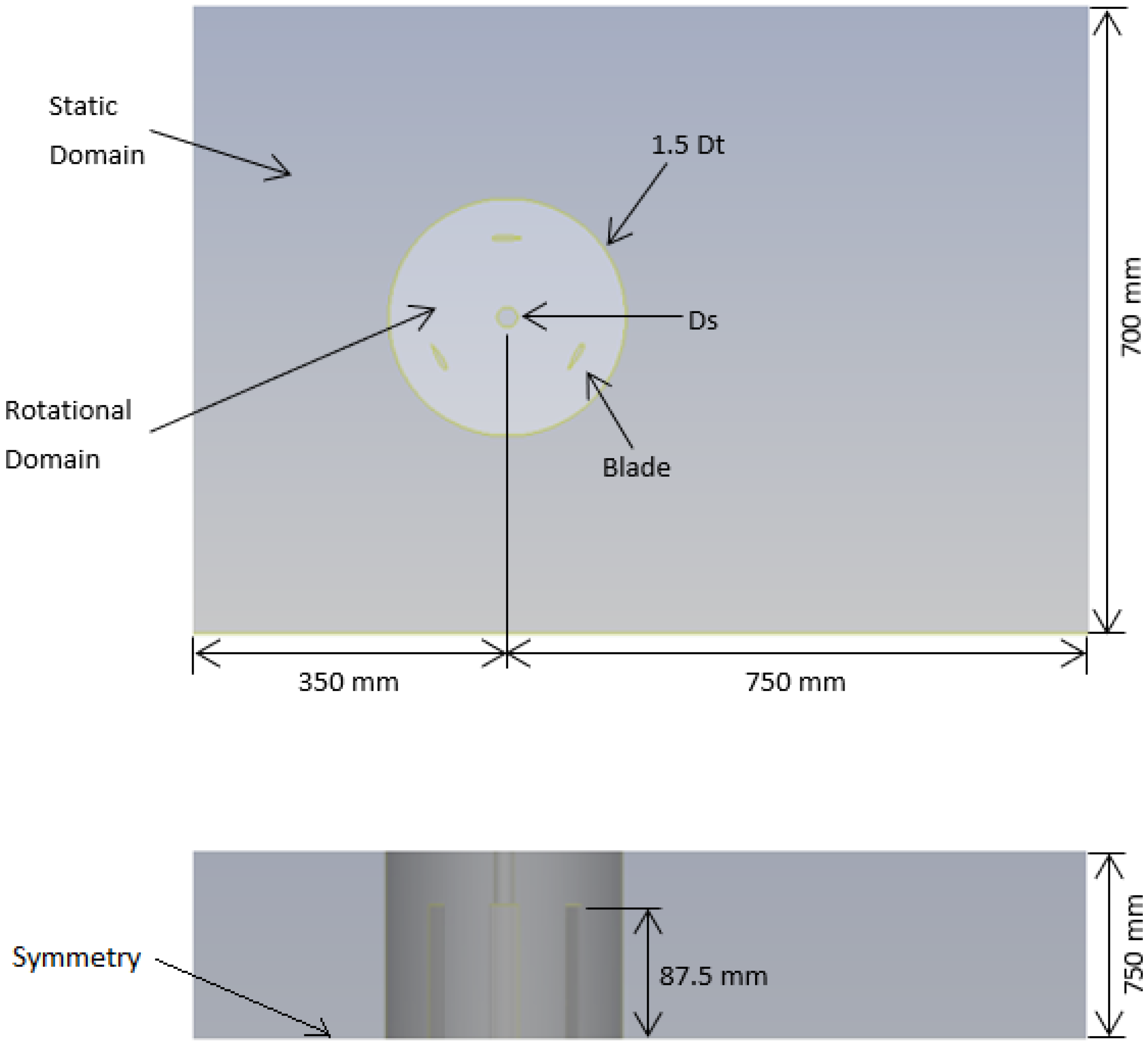
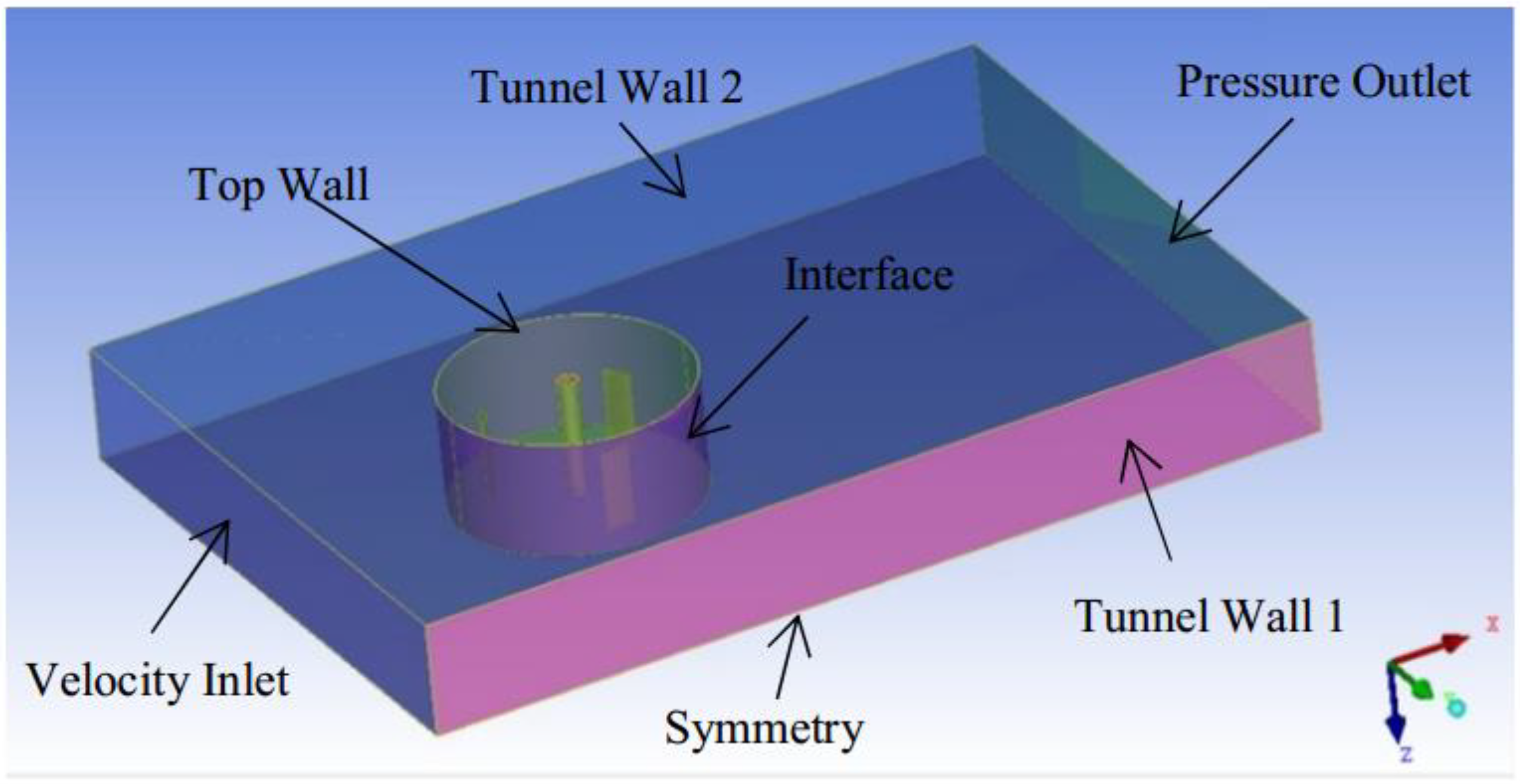
3.1. Computational Domain

Figure 1 shows the computational domain used in the present study. In the computational model, some geometric details such as blade supports and other turbine accessories that influence the overall turbine performance were omitted. This simplification was assumed in order to reduce the computational cost during the simulations. Additionally, only half of the domain was generated, and the condition of symmetry was established in the model. The symmetry is defined at the bottom surface of the computational domain as indicated in Figure 1. It is acknowledged that the assumption of symmetry in the model, especially for the hybrid RANS-LES simulations is a very strong assumption due to the 3D characteristics of turbulent flow. The use of this kind of boundary condition suppresses turbulent fluctuations, especially in such an important plane (mid plane) of the flow. The reason for implementing a symmetry in the model is only to reduce the computational cost of the simulation. It is important to mention that the computational domain is divided in two: a rotating (cylinder) of 1.5 times turbine diameter and another static domain with the same dimensions of the hydrodynamic tunnel (see Figure 1). This is done in order to implement the sliding mesh technique and to simulate the rotation of the turbine at a constant angular velocity.

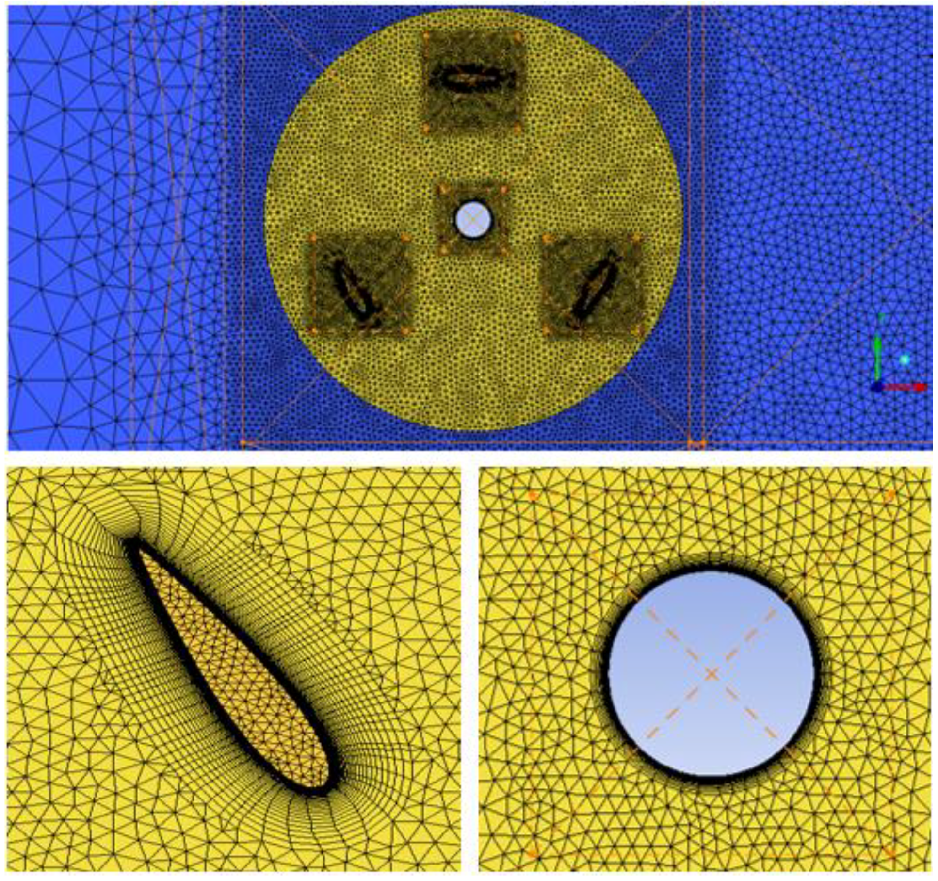
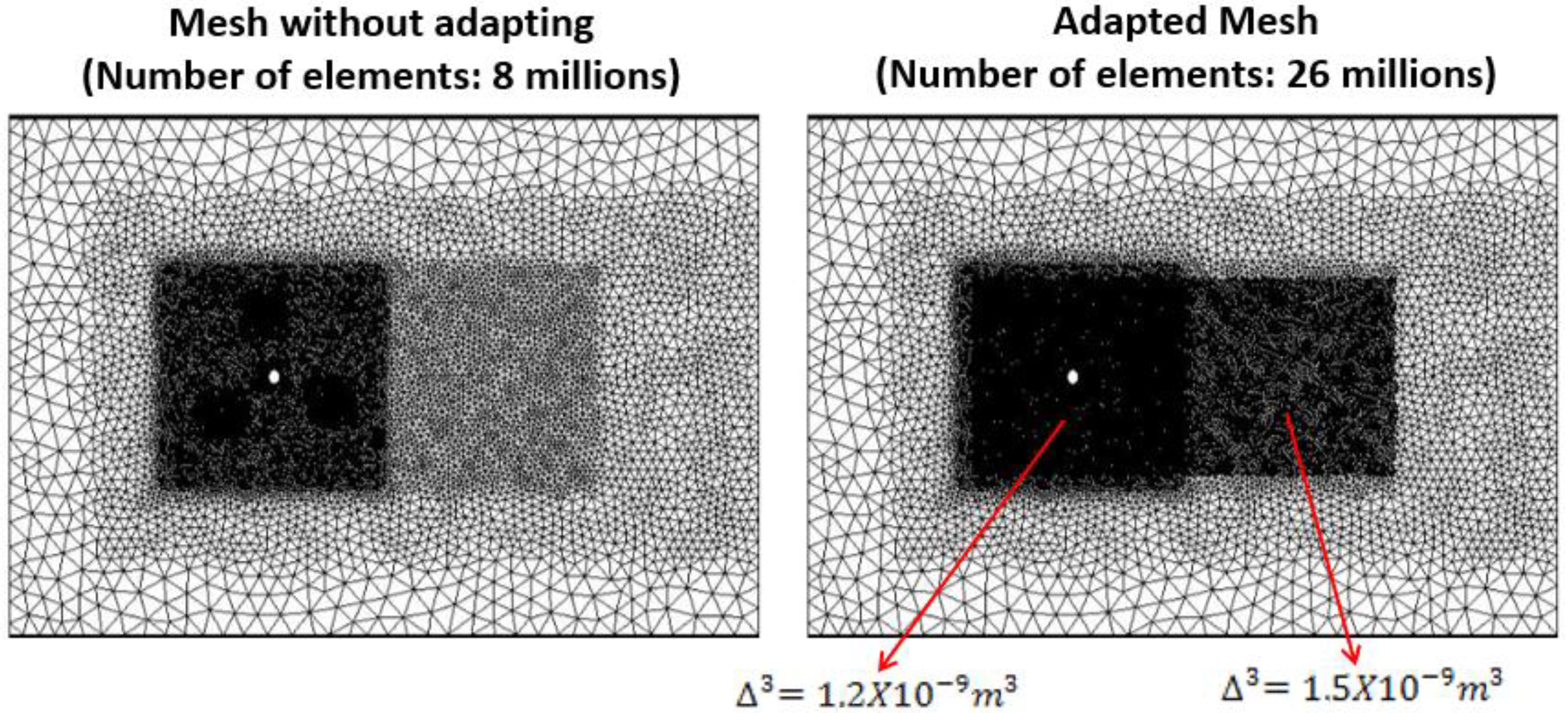
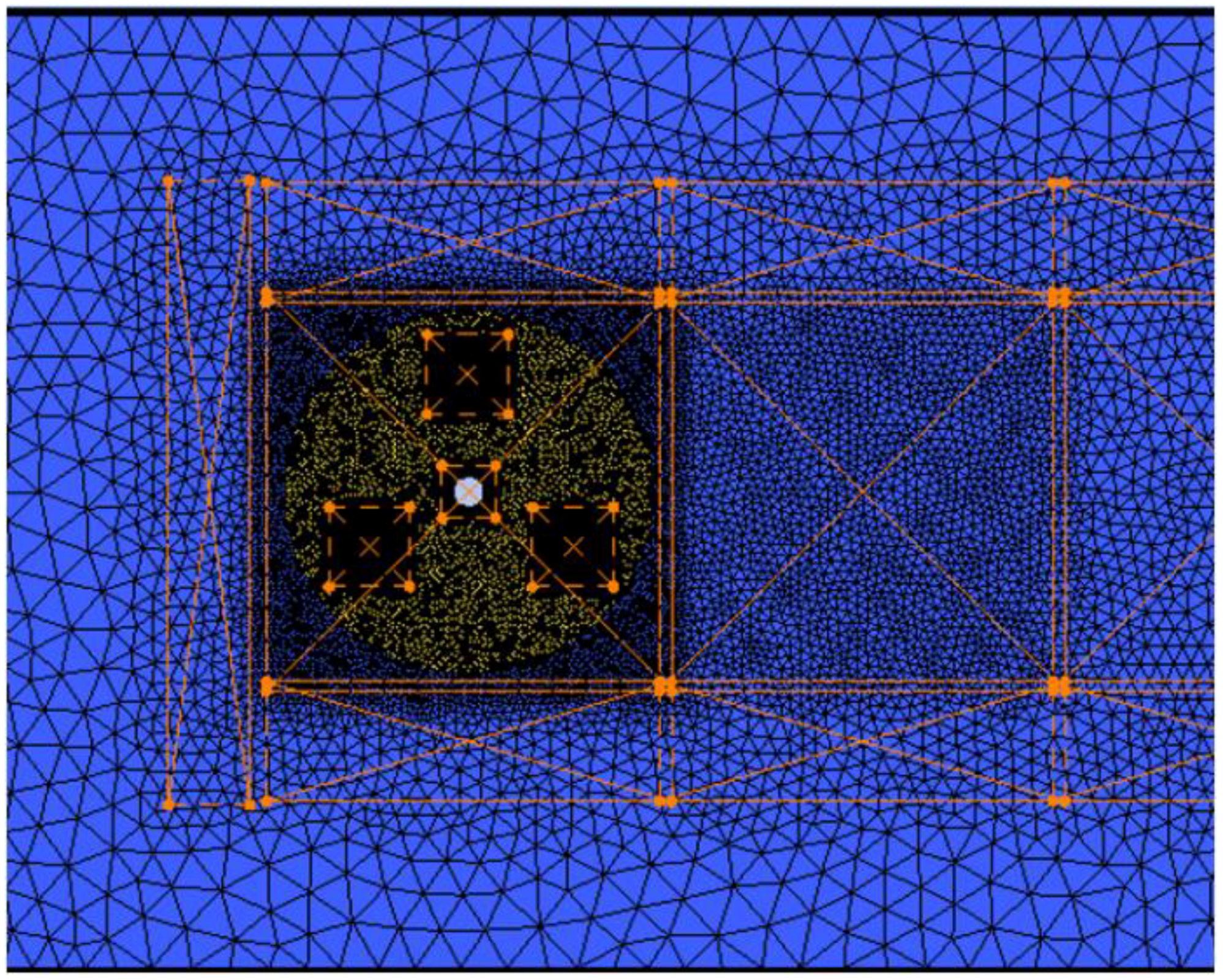
3.2. Mesh Generation

Four non-structured meshes were built using the commercial software ANSYS-ICEM and taking into account the parameters shown in

Table 1. Parameters for different mesh sizes close to the blades.

Mesh Size	First Row Thickness (mm)	Growth Rate	Number of Layers	Number of Elements	Average Y+ at the Blades	Average Power Coefficient $\left(\overline{{\mathit{C}}_{\mathit{P}}}\right)$
Coarse (M4)	0.106	1.1	17	514,741	16.12	0.412
Medium (M3)	0.015	1.1	40	3,954,000	2.15	0.440
Fine (M2)	0.005	1.12	45	8,016,441	0.73	0.457
Extrafine (M1)	0.003	1.12	50	11,355,960	0.43	0.463

. The meshes were constructed with prismatic elements on the surface of the turbine blades, to correctly capture the turbulent boundary layer around the blades (Figure 2).

It is clear the fine and extra fine meshes satisfy the criterion of y+ less than 1 at the blades surface (where $y+=\frac{y\sqrt{\frac{{\tau }_{wall}}{\rho }}}{\vartheta }$; $y$ is the distance to the wall, ${\tau }_{wall}$ is the shear stress at the wall, $\rho$ is the density and $\vartheta$ is the kinematic viscosity). Satisfying this criterion implies that numerically the turbulent boundary layer is completely resolved, since the first cell of the mesh close to the blades is within the viscous sublayer. This requirement is also important in order to correctly predict the shear stresses and the forces over the blades. The rest of the domain was meshed with tetrahedral elements and no refinements were used at the tunnel walls. The boxes of densities (described by orange lines in Figure 3) were used to have a higher resolution in the zones of influence of the turbine as the wake and the surroundings of the blades, and also to ensure a less abrupt transition in the element size between near and far fields.

3.3. URANS k-ω SST Simulation Set-Up

The commercial software ANSYS-FLUENT v17 was used for the present work. Regarding boundary conditions (see Figure 4) on the velocity inlet was assigned a velocity of 2.8 m/s and a turbulence intensity of 2% which correspond to the values originally used by Amet [12]. It is important to mention that no experimental measurements are reported of the turbulence intensity for the water tunnel used at LEGI.

The Reynolds number based on the chord length (Re) is given by:

$$Re=\frac{\rho C\omega R}{\mu }=\lambda \frac{\rho C{U}_{\infty }}{\mu }$$

(1)

where $\rho$ is the density of water, C is the chord length, µ the water dynamic viscosity and $U_{\infty }$ is the free stream velocity and ω is the angular velocity of the turbine. The TSR (λ) is the relation between the tangential velocity at the tip of the blade and the free stream velocity ($U_{\infty }$) and is defined as:

$$\lambda =\frac{\omega R}{U_{\infty }}$$

(2)

The Reynolds number when λ is equal to 2 is 1.2 × 10⁵. A constant value of 0 Pa was imposed on the pressure outlet. On the lateral and bottom walls the non-slip wall condition was used. The condition of symmetry was assigned to the upper surface of the domain. The non-slip wall condition was used on the shaft and the turbine blades. In the rotating domain, the counterclockwise rotation velocity was changed as a function of the tip speed ratio being ω = 32 rad/s for λ = 1, ω = 64 rad/s for λ = 2, and ω = 80 rad/s for λ = 2.5. An interface condition was imposed between surfaces of the static zone and the zone with rotation in order to guarantee the continuity of mass and momentum fluxes. The time step was set equal to 2.72 × 10⁻⁴ s, corresponding to a rotation angle ∆θ = 1 deg. Regarding space discretization, a second order upwind scheme was used for the convective terms. A number of iterations per time step (75) were performed and the velocity–pressure coupling parameter was handled with the SIMPLE method.

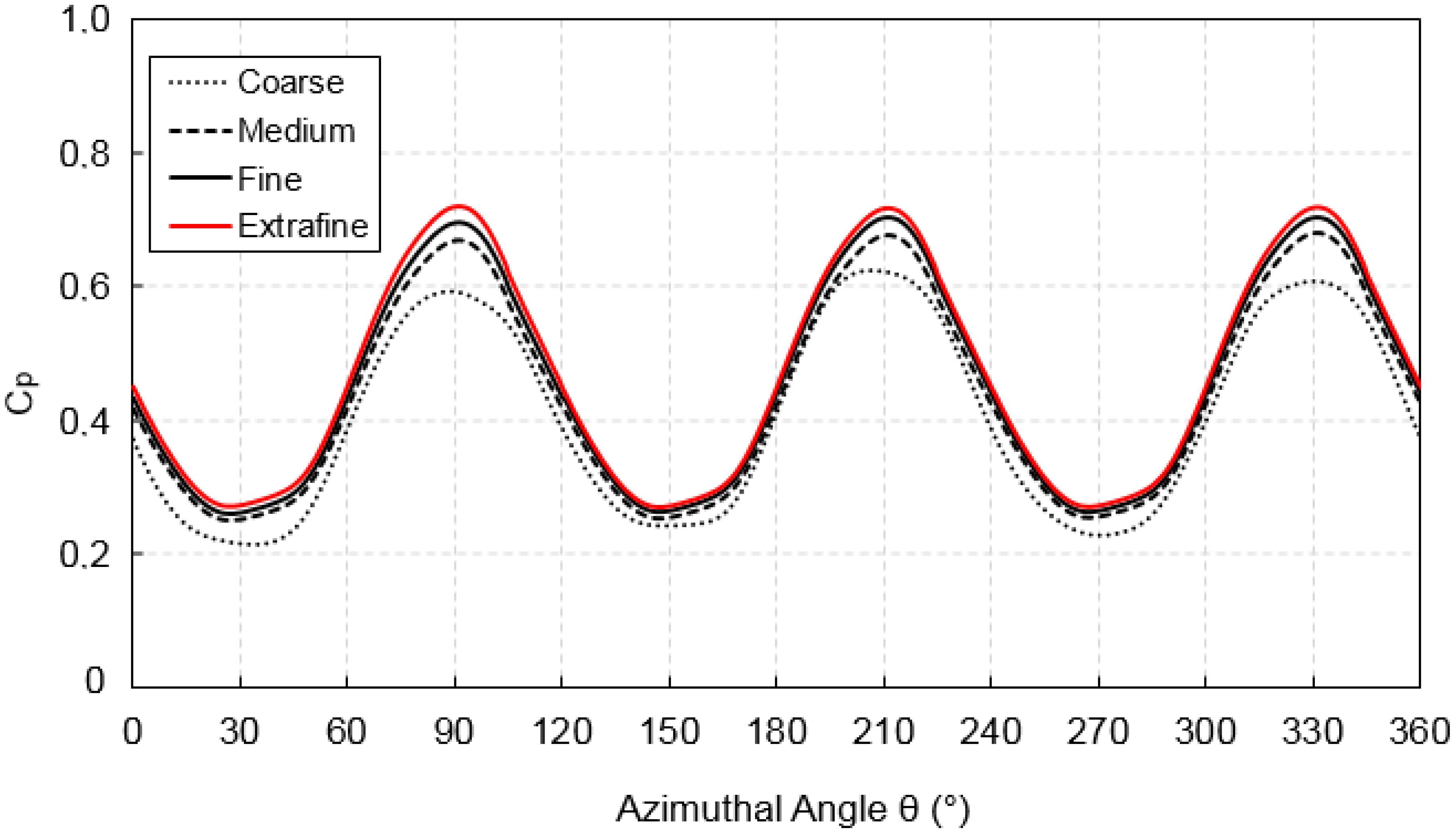
4. URANS Model Convergence

The four meshes shown in Table 1 were used for the validation study and the average power coefficient $\left(\overline{C_P}\right)$ is the key variable of interest for this study. The total instantaneous power coefficient is defined as:

$$C_p=\frac{T\omega }{\rho HR{U}_{\infty }^3}$$

(3)

where T is the hydraulic torque exerted on the turbine. The power coefficient was averaged by integrating the instantaneous values on a revolution by the following equation:

$$\overline{C_p}=\left(\frac{1}{2\pi }\right){{\displaystyle \int }}_0^{2\pi }{C}_{p}d\theta$$

(4)

The average power coefficient ($\overline{C_P}$) of the turbine at a tip speed ratio of λ = 2 was used as convergence criteria. The average power coefficient was calculated in the last revolution (5th) of the turbine when the evolution of $C_p$ achieved a periodic behaviour (Figure 5). It is clear that when the mesh is refined, $\overline{C_P}$ values converge, showing a difference between the fine and extrafine meshes of less than 2%.

In this study, grid convergence analysis was performed using three meshes (M3, M2 and M1) with the specifications given in Table 1. The final results of the convergence analysis using the generalized Richardson extrapolation method [13] are summarized in

Table 2. Summary of the Richarson extrapolation.

Mesh Sizes	Calculated Order of Accuracy (p)	Apparent Convergence Condition $\left({\mathit{R}}^{*}\right)$	${\overline{{\mathit{C}}_{\mathit{P}}}}_{\mathit{e}\mathit{x}\mathit{a}\mathit{c}\mathit{t}}$	Grid Convergence Index
M3 M2 M1	1.87	0.353	0.487	0.031

. It is clear that the numerical results are in the convergence region.

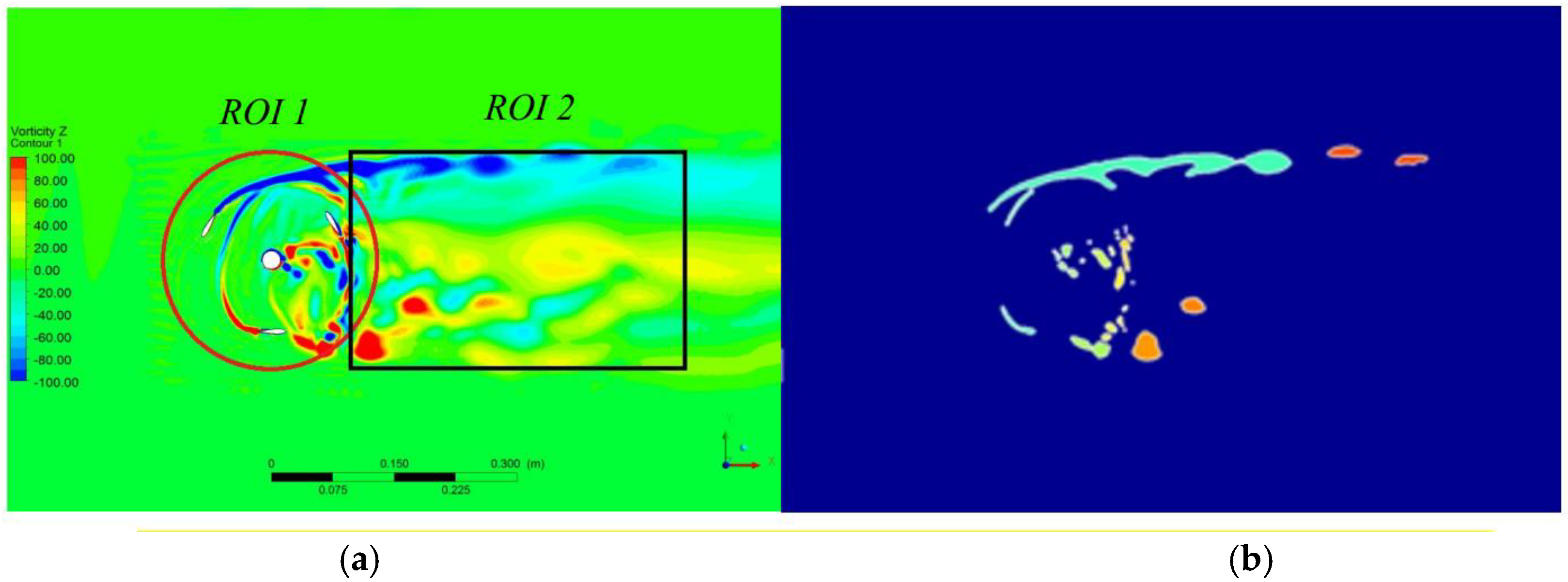
5. DES Model Adaptation

The DES model is a combination of the RANS and LES models, the aim of this is to treat the boundary layer with RANS and to capture the outer detached vortices with LES [14,15]. The mesh adaption process to use the DES model was made taking into account that the flow field can be divided into three basic regions: Euler Region, RANS Region and LES Region [16].

For the refinements of the LES region and the so-called grey areas, an estimation of the LES filter was performed based on what has been reported in the literature [16]. To perform this procedure, the LES filter was initially approximated by dividing the characteristic length of the blade (blade chord length) 30 times, giving a LES filter value of Δ = 0.00106 m, which is less than ∅_min = 0.003 m, the diameter of the smallest vortex captured in the fine mesh. The smallest diameter of the vortices was captured in the region of interest (ROI) by an image processing algorithm developed in MATLAB (Figure 6).

The objective of the algorithm is to filter the vortices shed by the blades in two ways, according to the intensity of the vorticity field in a plane and a geometric threshold. The threshold allows to identify vortices with a roughly circular or spiral pattern [17]. When the threshold is equal to 1 the algorithm identifies a vortex with a circular shape and as it decreases, vortices with spiral shape begin to be identified.

The measurement of the diameter of the vortices was performed in five planes along the span of the turbine, looking for the smallest vortex in the wake of the blades and the turbine. With the LES filter value of ∆ = 0.00106 m, the volume of refinement of the cells (∆³ = 1.2 × 10⁻⁹ m³) was estimated. Taking into account the computational cost of the simulations and to ensure a smooth transition between elements of the rotating domain and those of the wake of the turbine, a cell volume size of ∆³ = 1.5 × 10⁻⁹ m³ was used in the far field. The adaptation of the DES mesh was made with these two volumes of refinement. The total number of elements of the adapted mesh was 26 million as shown in Figure 7.

For the temporal resolution, the time step of the URANS simulations was recalculated under the assumption that more precision than stability is required within the DES model simulations. The time step is calculated according to Spalart [16] as ∆t = ∆/U_max = ∆/1.5U_∞ = 2.4 × 10⁻⁴ s, where U_max, is the maximum velocity registered in the simulations, which in this case is approximately 1.5 times the velocity of the incident fluid flow.

6. Results

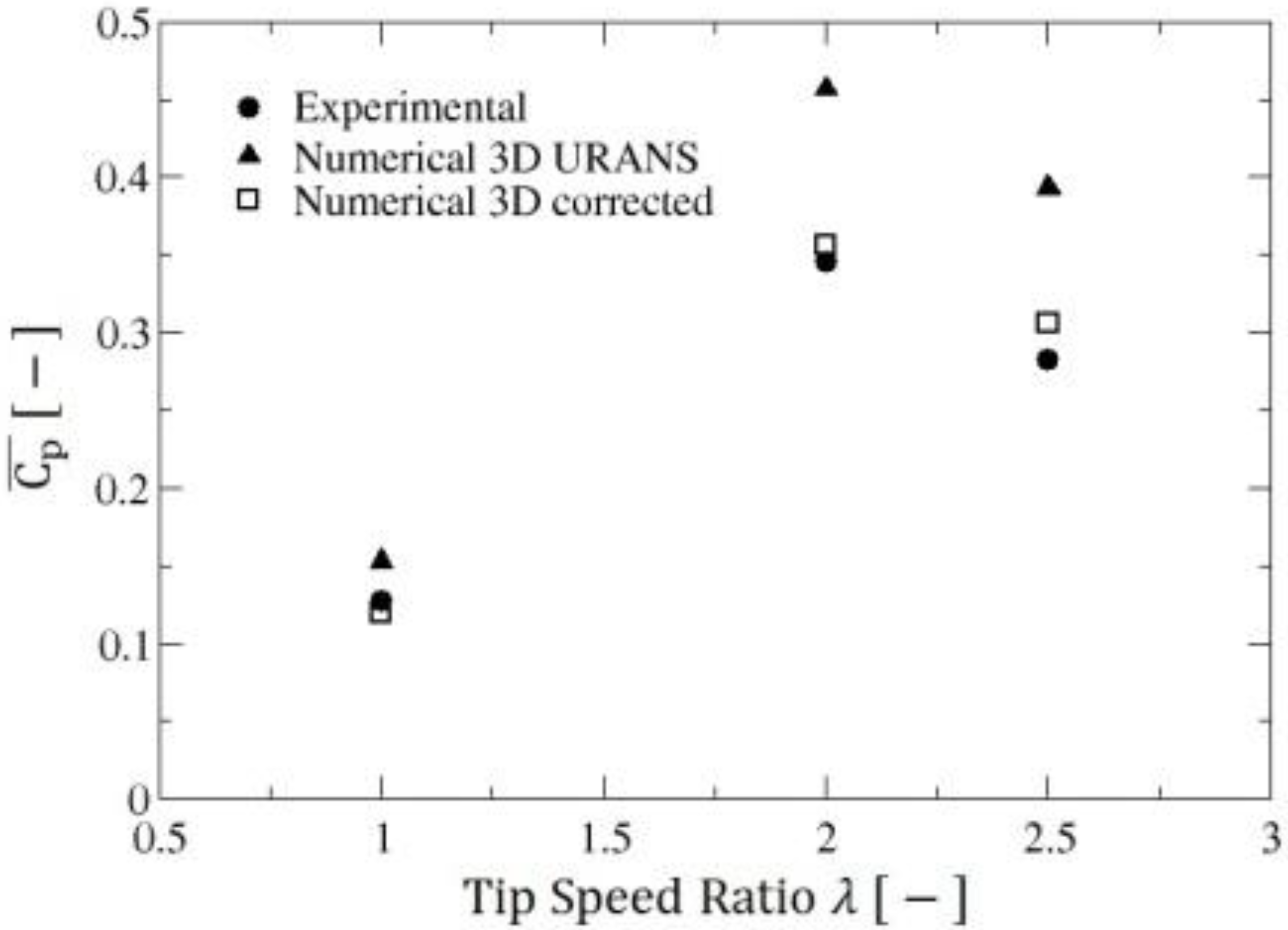
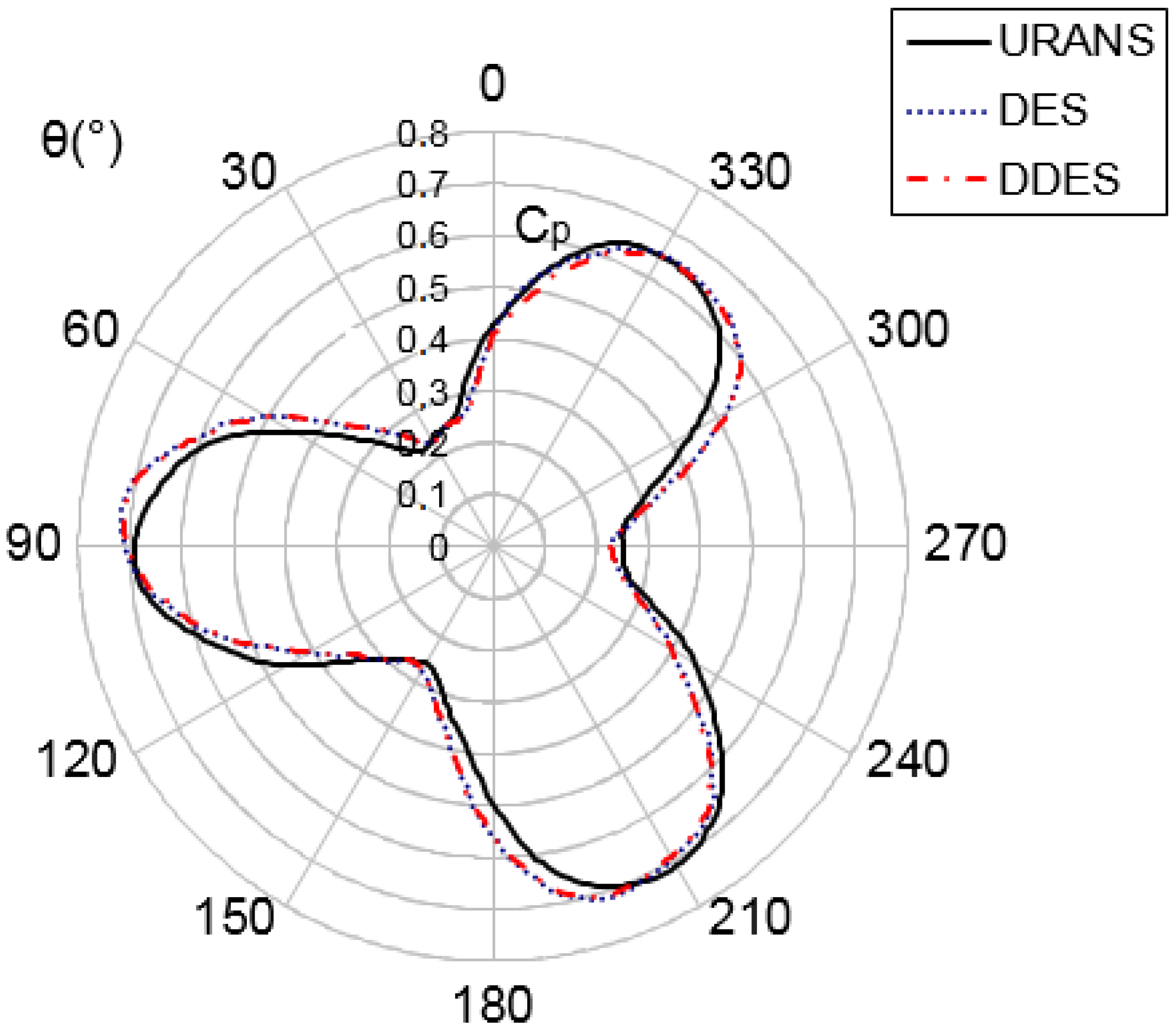
6.1. Power Coefficient

The power coefficient calculation of the turbine was performed for three different TSR, in order to compare the results with experimental data. Figure 8 shows Cp for several instantaneous positions of the turbine; the highest Cp for the three TSR values is found at the azimuthal positions of 330°, 210° and 90°, and the lowest one at 30°, 150° and 270°.

Table 3. Comparison of experimental results of the average power coefficient with the URANS numerical simulations at different λ.

λ	$\overline{\mathit{C}\mathit{p}}$ Exp	$\overline{\mathit{C}\mathit{p}}$ Num 3D [11]	$\overline{\mathit{C}\mathit{p}}$ Num 3D
1	0.127	0.055	0.153
2	0.345	0.460	0.457
2.5	0.282	-	0.393

shows the comparison of numerical results of the simulations for three different TSR with respect to the experimental and numerical results reported by Pellone et al. [11].

It is clear the large differences are observed between the numerical and experimental results, nevertheless the results of the present work show better agreement that the results obtained by Pellone et al. [11]. In the 3D URANS numerical simulations performed by Pellone et al. [11] and referenced by [9], the Cp average results of the same turbine used in the present study with and without the struts were compared against the experimental results only for λ = 2. The Cp average of the turbine without struts overestimate the Cp average prediction around 22%, in contrast the turbine with struts leads to an average Cp very close to the experimental value. The scope of the present numerical research does not include the evaluation of the effect of the struts in the average Cp because the struts also need a fine grid resolution at the wall (Y+ values less than 2), which would increase the computational costs of the simulations especially for the hybrid RANS-LES models.

Figure 9 shows that for the three TSR the numerical results overestimate the values of the $\overline{C_P}$ with regard to those obtained in experimentation. However, if such values are corrected with the estimated loss due to the supporting arms [9], the corresponding points are much closer to the experiments (hollow squares in Figure 9). Figure 10 shows that a difference of less than 1% is obtained between the averaged Cp predicted by URANS and the hybrid models. Small differences are observed at azimuthal angles close to 90°, 210° and 300° in which massive separation (dynamic stall) is occurring in the blades. These small differences are explained by the capabilities of the hybrid RANS-LES models to capture massively separated flows and to better predict the instantaneous forces at these azimuthal angles.

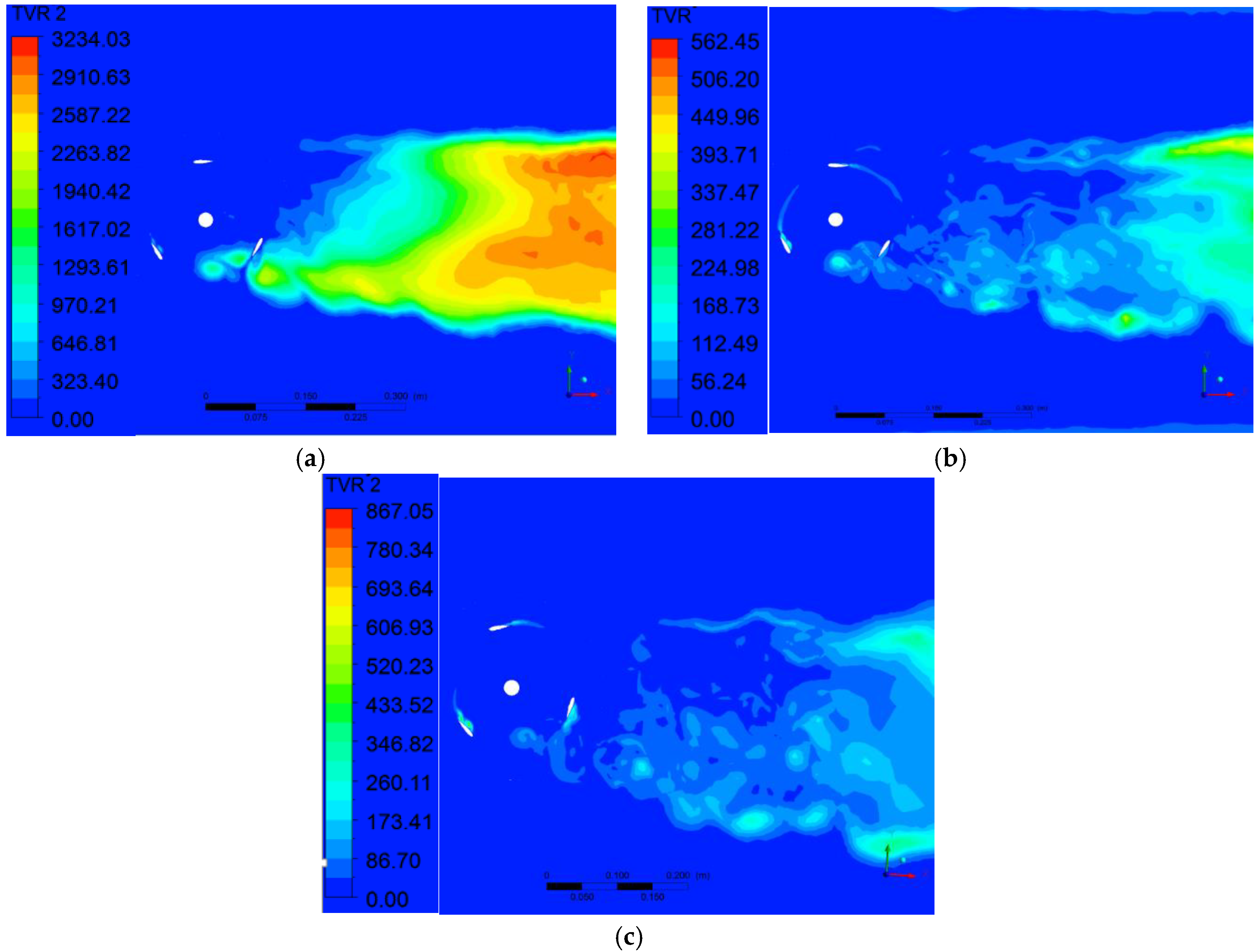
6.2. Turbulent Viscosity Ratio (TVR)

Figure 11 shows the instantaneous contours of turbulent viscosity ratio (TVR) for the three numerical models implemented in this study. For the DES and DDES model, it can be observed that TVR presents a great reduction, specifically in the near wake, when compared to URANS.

This reduction in the magnitude of the TVR is due to the treatment of the production term of the transport equations of the DES and DDES models when the mesh has the proper refinement. By having this behaviour in the DES and DDES models, it is possible to identify more turbulent scales in the near and distant wake of the turbine that are not appreciable in the URANS model.

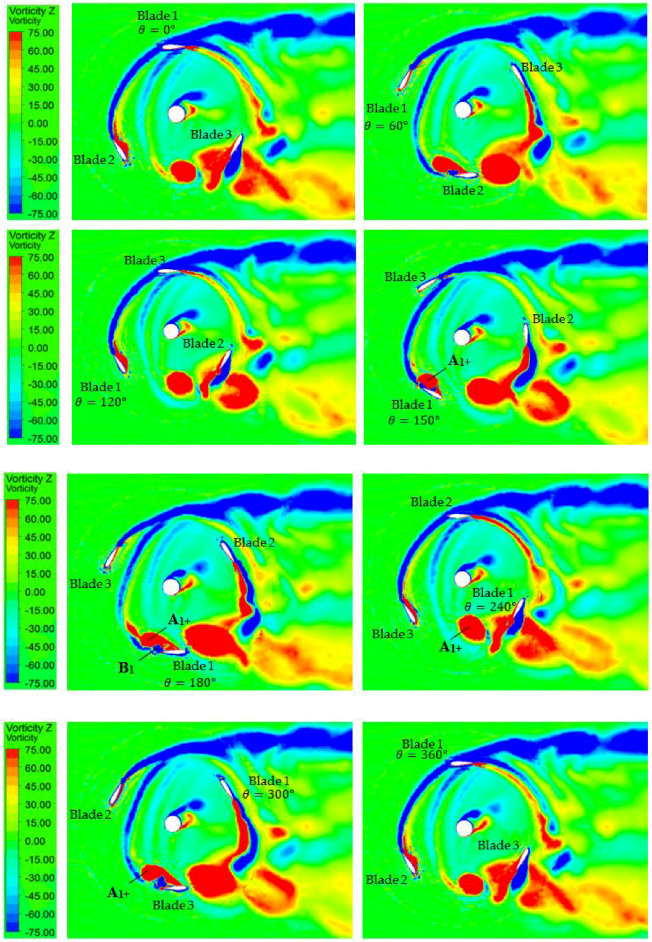
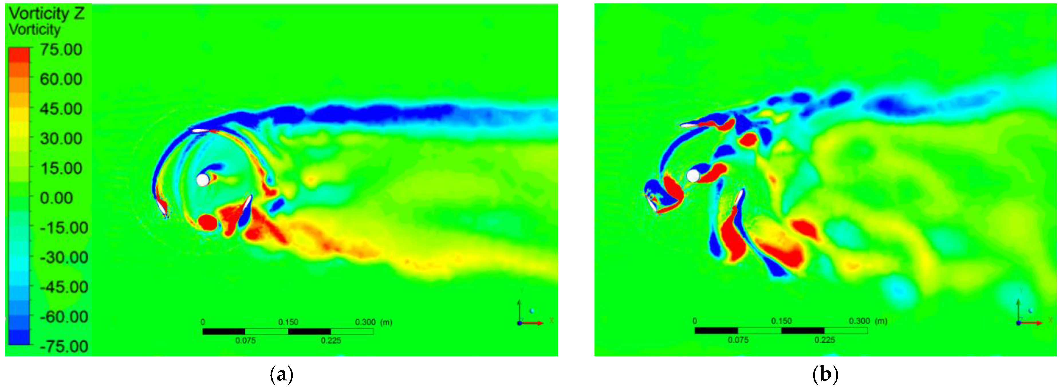
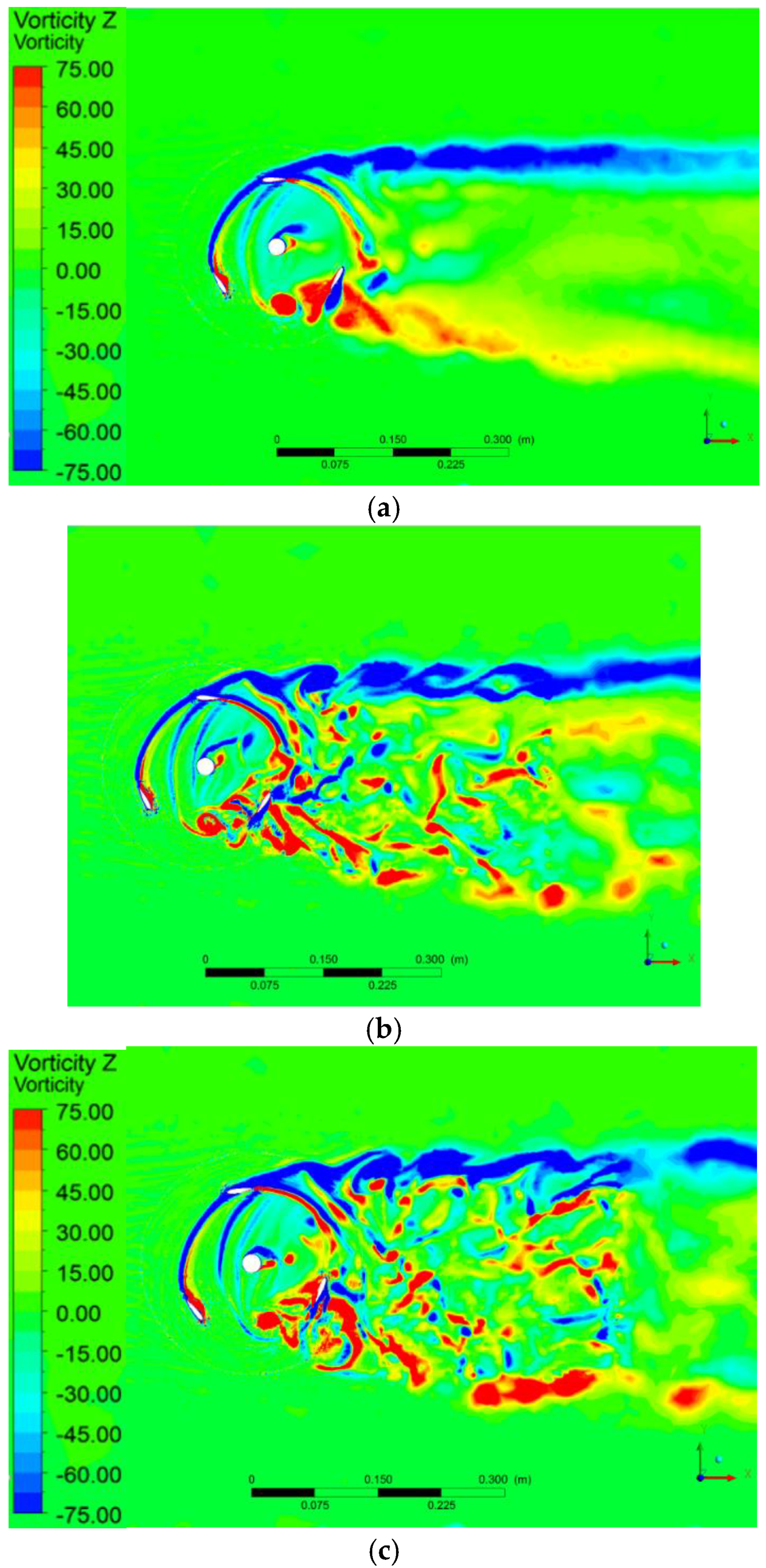
6.3. Vorticity Field

In Figure 12 the evolution of vortices detached from the turbine blades can be observed at six different azimuth angles (θ) in the plane of symmetry for the URANS turbulence model at λ = 2. For this case there is a strong detachment of vortices when the angle of attack increases, generating vortices at the leading edge of the blades that are transported along the blades and downstream of the turbine as in dynamic stall. The vortices that detach from the turbine blades (Figure 12), have higher intensity in the zone between the azimuthal angles θ = 150° and θ = 270°, in this zone the vortices of larger scale are convected downstream of the turbine and interact with the other blades.

Between an azimuthal angle of θ = 0° and θ = 80°, the flow is attached but at θ = 90° the flow separation from the leading edge of the blade starts. As the turbine rotates, an initial vortex is generated at the trailing edge of the Blade 1, called A1+ (Figure 12), which begins to roll at θ = 150° and circulates around the blade profile. Vortex A1+ is completely detached from the trailing edge when at θ = 210° azimuthal position. From this point the vortex A1+ is convected, increasing its intensity downstream of the turbine by the interaction and possible stretching generated with the vortices shed at the trailing edge of Blade 1 at θ = 240°. This happens until the Blade 3 impacts it and divides the vortex A1+ into two vortices that dissipate further downstream of the turbine. From Figure 12, it can also be seen that at θ = 180° for Blade 1 there is a counter-rotating vortex (B1−) which is shed from the trailing edge of the blade and dissipates rapidly in the same area of the turbine rotor.

A characteristic phenomenon of the operation of the vertical axis turbines is the dynamic stall which occurs at low TSR, and impacts turbine performance [7]. In order to understand how the phenomenon of dynamic stall of the turbine at different tip speed ratios occurs, contours of the vorticity field in the plane of symmetry for the URANS model were obtained (Figure 13).

At λ = 1, large vortices are shed from the blades due to the high angles of attack experienced at low λ, these vortices shed from the blades are convected downstream, impacting on the blades as they rotate, reducing blade performance and the generated torque. For the case λ = 2 there is a significant reduction in the size of the shed vortices due to the increase in the angular velocity of the blades with respect to the incident velocity. This reduction in the size of the vortices improves the performance and increases the torque generated by the turbine. It is also clear that the wake (far field) of the turbine is wider at λ = 1 than at λ = 2.

In Figure 14, the behaviour of the vorticity field in the plane of symmetry for the three turbulence models (URANS, DES and DDES) is shown for λ = 2. In all three models there are similar characteristics such as the length of the distant wake and the trajectory of the flow of the vortices with negative magnitude that appear along the wake.

Although the RANS model defines the main vortices that are generated around the blades and at the top and bottom of the turbine wake, this model does not accurately describe their intensity, much less their propagation and dissipation downstream of the turbine. In the DES and DDES model, unlike the URANS model, a larger number of vortices can be observed in the wake. The largest vortices are present in the rotor area, whereas further back in the wake smaller vortices are appreciated.

From Figure 14, it can also be observed that the expansion of the wake in the three models is smaller in the upper part than in the lower one. As a fact the vortices that emerge from the upper part, θ = 270° to θ = 90°, are weaker, whereas in the lower part, where the intensity and generation of vortices is stronger, the expansion of the wake is faster.

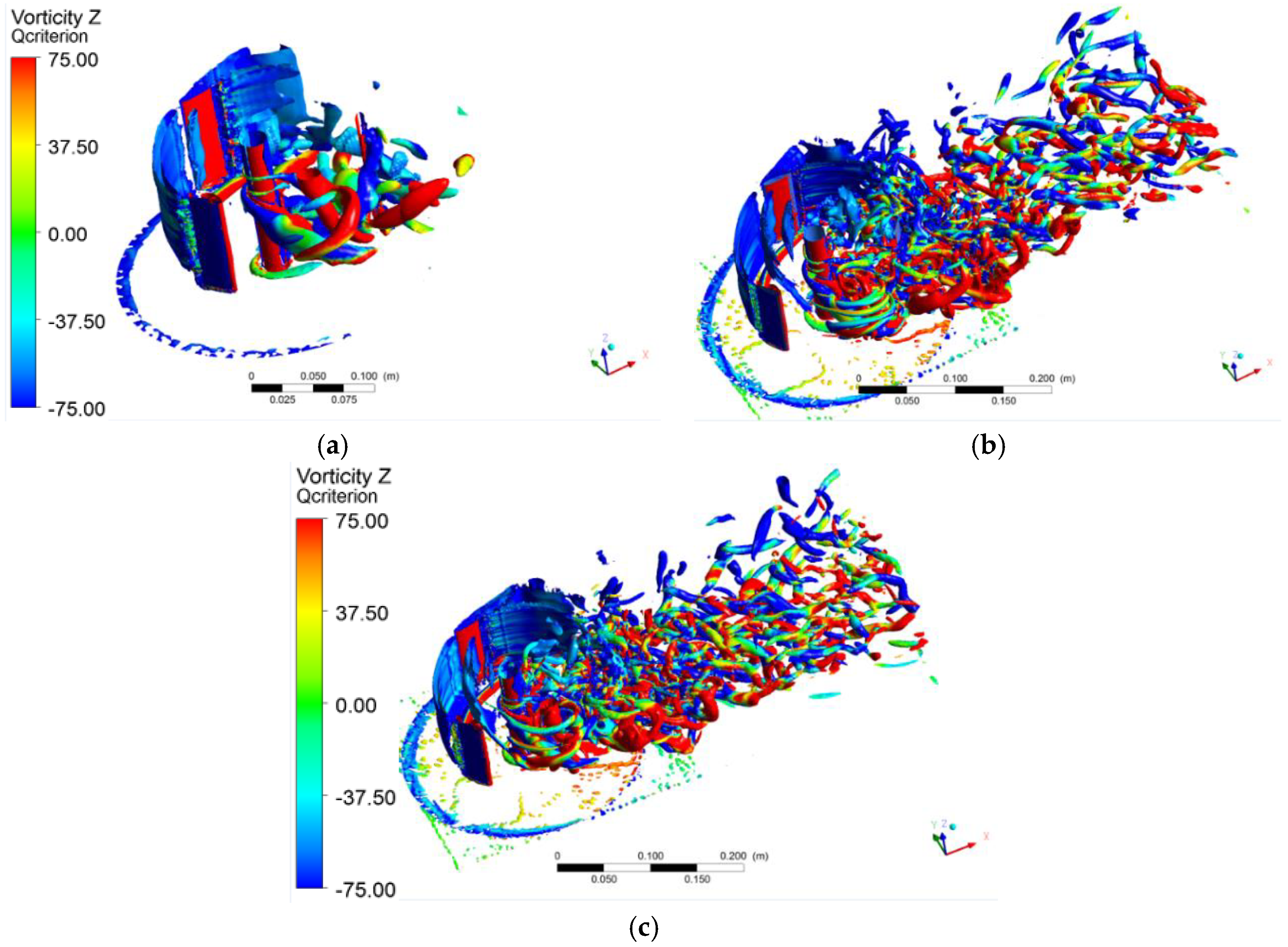
6.4. 3D Visualization of Vortex Structures Using Q-Criterion

The Q-criterion is used to identify vortex structures in a flow field, generated by the interaction of fluid with solid surfaces. The Q-criterion is the second invariant of the velocity gradient across the flow field, and its objective is to identify a vortex in the zone where the second invariant of the velocity gradient tensor is positive and also the local pressure at that same point is less than the reference pressure [18]. This allows having more detail of the flow dynamics as opposed to what can be observed in a field contour of vorticity on a slice plane, since the dynamics of the vortices is a purely 3D phenomenon.

The stretching that the vortices undergo regarding their initial shape is associated with an increase of the vorticity component in the same direction of the stretching due to the principle of conservation of angular momentum.

An increase in the frequency of production of the vortices arising from the blades between θ = 180° and θ = 270° is observed for the DES and DDES models when compared to URANS. When the blades are between 90° and 270° a reduction in the intensity and length of the tip vortices generated at the trailing edge is evidenced; such decrease is associated with the variation of the lift experienced by the blades as they rotate by their different angular positions. DES and DDES models (Figure 15) allow better visualization of the phenomenon of vorticity in the wake. This is because with the filter applied in the mesh adaptation process in the LES zone, more vortices are resolved properly and a smaller number of them are modelled. In this case, calculation time increases. However, the obtained result is likely more accurate.

6.5. Computational Costs

To perform the simulation of the three turbulence models, 48 parallel Intel XEON E5620 processor cores and 96 GB of RAM were used. It is important to mention that these resources were dedicated that means that during the simulations they were used exclusively to carry out the described simulations.

Table 4. Computational cost per rotation of the turbine for different turbulence models.

Turbulence Model	Number of Time Steps	Number of Iterations	Total Number of Iterations	Iteration Time (s)	Simulation Time (days)
URANS	1800	75	135000	6.4	~10
DES	2060	75	154500	16.4	~30
DDES	2060	75	154500	16.4	~30

summarizes the computational cost of the different turbulence models used in the present study per rotation of the turbine for λ = 2.

7. Conclusions

A detailed 3D analysis of the flow around a Darrieus (H type) turbine in confined flow conditions in a water tunnel was presented. The performance of the turbine and the flow dynamics were investigated through numerical simulation employing the URANS, DES and DDES turbulence models, all of them based on k-ω SST. The numerical results of the URANS model for the three TSR studied (λ = 1, λ = 2 and λ = 2.5) show a similar behaviour to that expected regarding the experimental power curve of the turbine.

As a result, hybrid DES and DDES models do not show much difference in the computed power coefficient of the turbine with respect to the URANS model. However, it is noticed that the 3D simulations made with a proper refinement of the mesh in the DES and DDES models allow to identify the different scales of the vortical structures and the turbulent flow phenomena present in the turbine wake that are not appreciable in the URANS model. These 3D structures and the associated phenomena in the wake are of great importance since their interaction with other elements of the turbine influence the decrease of the overall performance of the turbine, produce noise and vibrations, all of them non-desirable effects to maintain the structural integrity of the device.

The results obtained in this study show that the URANS model based on k-ω SST model predicts very well the overall performance of the turbine with lower computational costs than either the DES or DDES models. Nevertheless, flow dynamics phenomena like blade tip vortex detachment, vortex stretching and the interaction of the vorticity structures with the blades and other components of the turbine are better resolved with hybrid models.

According to the results found in the experimentation and as found in this computational study, it is observed that the optimal operation speed happens close to λ = 2. The evaluation of the vorticity field in this tip speed ratio shows that the detached vortices in the blades and the shaft are smaller than the detached ones in the case λ = 1. For such a low λ, the dynamic stall phenomena are happening and therefore the turbine global performance decreases.

The prediction of the overall efficiency of the turbine can be improved if the turbine arms are added to the 3D CFD model [11]. Previous studies have shown that the drag force generated by these elements influence the decrease of the average C_P and the generated torque; it is important to consider them also at the design step since modifications in the geometry of these elements would help to increase the efficiency of the turbine [19].

References

1. Hall, T.J. Numerical Simulation of a Cross Flow Marine Hydrokinetic Turbine. Master’s Thesis, University of Washigton, Seattle, WA, USA, 2012. [Google Scholar]
2. Antheaume, S.; Maitre, T.; Achard, J. Hydraulic darrieus turbines efficiency for free fluid flow conditions versus power farms conditions. Renew. Energies 2008, 33, 2186–2198. [Google Scholar] [CrossRef]
3. Dai, Y.M.; Lam, W. Numerical Study of Straight-bladed Darrieus-type Tidal Turbine. ICE Energy 2009, 162, 67–76. [Google Scholar] [CrossRef]
4. Lain, S.; Osorio, C. Simulation and Evaluation of a Straight-bladed Darrieus-type Cross Flow Marine Turbine. J. Sci. Ind. Res. (JSIR) 2010, 69, 906–912. [Google Scholar]
5. Nabavi, Y. Numerical Study of the Ducted Shape Effect on the Performance of a Ducted Vertical Axis Tidal Turbine. Master’s Thesis, The University of British Columbia, Vancouver, BC, Canada, 2008. [Google Scholar]
6. Rawlings, G.W. Parametric Characterization of an Experimental Vertical Axis Hydro Turbine. Master’s Thesis, The University of British Columbia, Vancouver, BC, Canada, 2008. [Google Scholar]
7. Ferreira, C.J.; Bijl, H.; van Bussel, G.; van Kuik, G. Simulating Dynamic Stall in a 2D VAWT: Modeling Strategy, Verification and Validation with Particle Image Velocimetry Data. J. Phys. Conf. Ser. 2007, 75, 012023. [Google Scholar] [CrossRef]
8. Lei, H.; Zhou, D.; Bao, Y.; Li, Y.; Han, Z. Three-dimensional Improved Delayed Detached Eddy Simulation of a two-bladed vertical axis wind turbine. Energy Convers. Manag. 2017, 133, 235–248. [Google Scholar] [CrossRef]
9. Maître, T.; Amet, E.; Pellone, C. Modeling of the Flow in a Darrieus Water Turbine: Wall Grid Refinement Analysis and Comparison with Experiments. Renew. Energy 2013, 51, 497–512. [Google Scholar] [CrossRef]
10. Marsh, P.; Ranmuthugala, D.; Penesis, I.; Thomas, G. Three Dimensional Numerical Simulations of a Straight-Bladed Vertical Axis Tidal Turbine. In Proceedings of the 18th Australasian Fluid Mechanics Conference, Launceston, Australia, 3–7 December 2012. [Google Scholar]
11. Pellone, C.; Maître, T.; Amet, E. 3D RANS Modeling of a Cross Flow Water Turbine. In Proceedings of the SimHydro: New Trends in Simulation Hydroinformatics and 3D modeling, Nice, France, 12–14 September 2012. [Google Scholar]
12. Amet, E. Simulation Numerique d’une Hydrolienne à Axe Vertical de Type Darrieus. Ph.D. Thesis, Institut Polytechnique Grenoble, Grenoble, France, 2009. [Google Scholar]
13. Eca, L.; Hoekstra, M. A Verification Exercise for Two 2-D Steady Incompressible Turbulent Flows. In Proceedings of the ECCOMAS European Congress on Computational Methods in Applied Sciences and Engineering, Jyväskylä, Finland, 24–28 July 2004. [Google Scholar]
14. Spalart, P.R.; Jou, W.-H.; Strelets, M.; Allmaras, S. Comments on the Feasibility of LES for Wings, and on a Hybrid RANS/LES Approach. In Proceedings of the Advances in DNS/LES, Ruston, LA, USA, 4–8 August 1997. [Google Scholar]
15. Shur, M.; Spalart, P.R.; Strelets, M.; Travin, A. Detached-eddy simulation of an airfoil at high angle of attack. In Proceedings of the Engineering Turbulence Modelling and Experiments-4, Corsica, France, 24–26 May 1999. [Google Scholar]
16. Spalart, P.R. Young-Person’s Guide to Detached-Eddy Simulation Grids; NASA/CR-2001-211032; NASA Langley Research Center: Hampton, VA, USA, 2001.
17. Bussiere, M. The Experimental Investigation of Vortex Wakes from Oscillating Airfoils. Master’s Thesis, University of Alberta, Edmonton, AB, Canada, 2012. [Google Scholar]
18. Gorle, J.M.; Chatellier, L.; Pons, F.; Ba, M. Flow and Performance analysis of H-Darrieus hydro turbine in a confined flow: A computational and experimental study. J. Fluids Struct. 2016, 66, 382–402. [Google Scholar] [CrossRef]
19. Marsh, P.; Ranmuthugala, D.; Penesis, I.; Thomas, G. Three-dimensional Numerical Simulations of a Straight-Bladed Vertical Axis Tidal Turbine Investigating Power Output, Torque Ripple and Mounting Forces. Renew. Energy 2015, 83, 67–77. [Google Scholar] [CrossRef]
Figure 1. Computational domain and turbine geometry.
Energies 11 02348 g001
Figure 2. Detail of the prism layer on the turbine blade and shaft.
Energies 11 02348 g002
Figure 3. Fine mesh with density box detail.
Energies 11 02348 g003
Figure 4. Nomenclature of the computational domain.
Energies 11 02348 g004
Figure 5. Grid convergence study for λ = 2.
Energies 11 02348 g005
Figure 6. (a) ROI in the instantaneous vorticity field on the symmetry plane for the URANS model, (b) Vortex capture by image processing in regions of interest in a vorticity contour.
Energies 11 02348 g006
Figure 7. Mesh adaptation to DES model.
Energies 11 02348 g007
Figure 8. Instantaneous power coefficient of the URANS model when λ = 1, λ = 2, λ = 2.5.
Energies 11 02348 g008
Figure 9. Average power coefficient for λ = 1, λ = 2, λ = 2.5. Numerical results vs. experiments.
Energies 11 02348 g009
Figure 10. Instantaneous power coefficient for the URANS, DES and DDES model.
Energies 11 02348 g010
Figure 11. Instantaneous turbulent viscosity field on the symmetry plane for the (a) URANS, (b) DES and (c) DDES models, at λ = 2.
Energies 11 02348 g011
Figure 12. Instantaneous vorticity field on the symmetry plane for the URANS model, at λ = 2, showing different azimuthal angles.
Energies 11 02348 g012
Figure 13. Instantaneous field of vorticity on symmetry plane for (a) λ = 1 and (b) λ = 2 for the URANS model.
Energies 11 02348 g013
Figure 14. Instantaneous vorticity field on the symmetry plane for the (a) URANS, (b) DES and (c) DDES models, at λ = 2.
Energies 11 02348 g014
Figure 15. Iso-surface contours of Q-criterion for the (a) URANS, (b) DES and (c) DDES models, at λ = 2.
Energies 11 02348 g015