Article

Modeling of Multiple Master–Slave Control under Island Microgrid and Stability Analysis Based on Control Parameter Configuration

1
Department of Electrical Engineering, North China Electric Power University, Baoding 071003, China
2
State Grid Jiaxing Power Supply Company, Jiaxing 314000, China
*
Author to whom correspondence should be addressed.
Energies 2018, 11(9), 2223; https://doi.org/10.3390/en11092223
Submission received: 16 July 2018 / Revised: 16 August 2018 / Accepted: 17 August 2018 / Published: 24 August 2018

Abstract

:
The stable operation of a microgrid is crucial to the integration of renewable energy sources. However, with the expansion of scale in electronic devices applied in the microgrid, the interaction between voltage source converters poses a great threat to system stability. In this paper, the model of a three-source microgrid with a multi master–slave control method in islanded mode is built first of all. Two sources out of three use droop control as the main control source, and another is a subordinate one with constant power control which is also known as real and reactive power (PQ) control. Then, the small signal decoupling control model and its stability discriminant equation are established combined with “virtual impedance”. To delve deeper into the interaction between converters, mutual influence of paralleled converters of two main control micro sources and their effect on system stability is explored from the perspective of control parameters. Finally, simulation and analysis are launched and the study serves as a reference for parameter setting of converters in a microgrid.

1. Introduction

Increasing exhaustion of fossil fuel and concerns about environmental pollution have led to extensive exploration of alternative energy sources. Of special interest are renewable energy sources (RES) such as solar and wind energy generation. This has resulted in the emergence of distributed generators (DGs) and the concept of microgrid (MG) has been introduced for proper utilization of DGs [1,2]. As different DGs have different characteristics and natural uncertainty, their presence can have negative effects on MG. Deviations of voltage and frequency are larger when MG operates in islanded mode in comparison with grid-connected mode [3,4]. Therefore, research on the stability of MG in islanded mode is of vital importance.
Usually, voltage source converters (VSCs) [5] are used to interconnect different DGs, whose output is mostly in the form of direct or non-common frequency alternating current. Although the increasing number of power electronic converters improves the control speed, it brings fuzzy influence on stability owing to the mutual influence between them [6]. To address the abovementioned issue, various methods have been proposed in the literature. In [7,8], the sensitivity of load voltage and voltage compensation term are introduced to control the bus voltage as well as improve the response speed and accuracy. However, limitations in applicable scope of load and voltage reduce its practicality. In [9,10], energy storage devices are used not only to suppress the transient power fluctuations, but also to greatly improve MGs’ stability thanks to a super-capacitor. However, this method affects the entire system and declines its inertia. In [11,12], a model that contains converters, controllers and alternating current (AC) grids is built, and high order state space expressions are formulated to determine its stability. However, the mutual influence between converters is neglected and a large number of equations make stability analysis more complex. To improve the accuracy of analysis, the model of MG has been improved for higher accuracy [13,14,15,16], including a linear model of MG combined with a boost converters model [13]; a global model ignoring the change in rotating angles and coupling terms between DGs [14]; a dynamic model of multi-module comprising multi-class of DGs and loads [15]; and a new type of small-signal model containing secondary control that analyzed the stability of the system with eigenvalue [16]. However, the models established in the above literature didn’t take into account the impact of electronic devices in grids. In view of this problem, some research delves deeper into the impact of control parameters on system stability [17]. It employs the root locus method to explore the reasonable ranges of control parameters by a small signal model. When multi-sources are paralleled, droop control can achieve coordination control without communication and the master–slave control method considers the power tracking of PV and wind power and the system stability [18,19]. However, the influence in different control parameters on the system is not considered, for their parameters are partly or almost the same.
In view of the problem in [18], this paper builds a model of multi-source MG, emphasizing the exploration of the mutual influence between converters on stability. To satisfy the decoupling condition, “virtual impedance” is introduced and a three-source decoupling small-signal model is built in addition to the characteristic polynomial also being deducted. On this basis, the mutual influence between converters on stability is analyzed on the level of control parameters by means of simulation studies. This method and the result can provide a reference for parameters’ configuration of converters in MG with a large number of electronic devices plugged in.

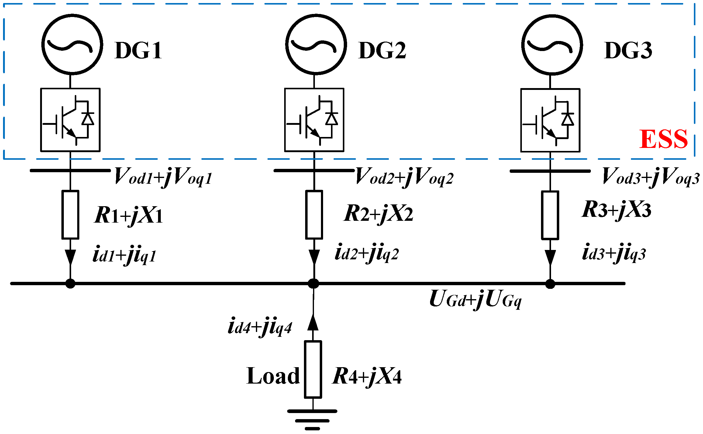
2. The Structure of Multi-Source Microgrid and Analysis of Its Problems

The diversity of DGs is a common feature of MGs [15]. Therefore, adopting appropriate control methods is an accurate and fast way to achieve the stable operation of islanded MG.

2.1. Multi Master–Slave Control Structure of MG

The traditional master–slave control method consists of one master controller and several slave controllers, which forms the energy supply system (ESS), in order to take into account the power tracking the renewable energy and the system stability [19]. With the increase in the permeability and scale of MG, however, a single master controller can no longer maintain the regulation of voltage and frequency. Hence, several master control sources should be set up with a droop control method. This solution is adopted in DGs (e.g., diesel engine, micro gas turbine, fuel cell, etc.), which regulate bus voltage and frequency. Relatively, photovoltaic and wind turbines with PQ control methods run as slave sources. The use of droop control alone implements the peer-to-peer control method, and it realizes the peer-to-peer control method, which can achieve local control and coordination control without communication.
Figure 1 shows a simplified structure of three-source MG in islanded mode. In Figure 1, Vodn + jVoqn and Rn + jXn are the output voltage of DGn and the equivalent impedance between bus and its converter; idn + jiqn is the output current of DGn (n = 1, 2, 3); UGd + jUGq is the bus voltage of MG. DG1 and DG2 serve as master controllers adopting a droop control method, embodying the flexibility and redundancy of a peer-to-peer control method in power vacancy allocation; DG3 serves as a slave controller adopting the PQ control method, ensuring its constant output in islanded mode; Load is comprised of resistance and reactance. This system adopts a master–slave control method when three DGs work and it adopts a peer-to-peer control method when DG3 quits running.

2.2. The Problem under Study

Fully symmetrical structure is mostly used in research on multi-source MG, whose parameters are the same in the same control method, ignoring the independence of control parameters of different DGs. The goal of this paper is to evaluate the following aspects: (1) whether there are interactions between control parameters to maintain stability when several converters operate in parallel; (2) whether there are interactions between control parameters of paralleled master controllers when a system’s control strategy changes from single master–slave control to multiple master–slave control method; and (3) how these interactions influence the stability of MG.
This paper verified the influence of droop coefficient difference on a multi master–slave control method based on the system model as shown in Figure 1. Set up the active droop coefficients of DG1, DG2 as 5 × 10⁻⁵, 10 × 10−5; and the reactive droop coefficients of them as 0.003; other parameter settings are shown in Appendix A; the waveform of bus voltage under different working conditions is shown in Figure 2. Figure 2a indicates the public bus bar voltage waveform when it works with DG1 and DG3, which contains only one master micro source; similarly, Figure 2b indicates the bus voltage waveform when it works with DG2 and DG3. The bus voltage can be kept stable in the two cases. Under the same coefficient setting, when DG1, DG2 and DG3 run together, the bus voltage waveform is oscillating and the microgrid is unstable as shown in Figure 2c. The cause of this phenomenon may be that the Cooperative operation of DG1 and DG2 makes the two controllers interact with each other, so that the operation of the microgrid is deviated from its stable running point, and then the instability occurs.
Based on this conjecture, this paper delves deep into the interaction between control parameters under multiple master controllers’ conditions, combining the case with the theoretical model.

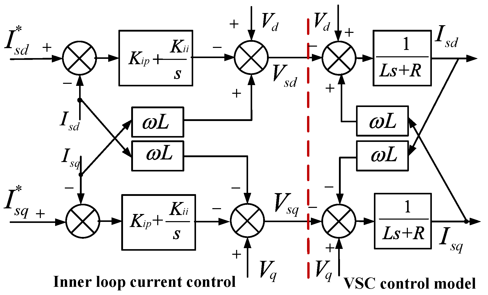
3. Theoretical Analysis of Control Methods

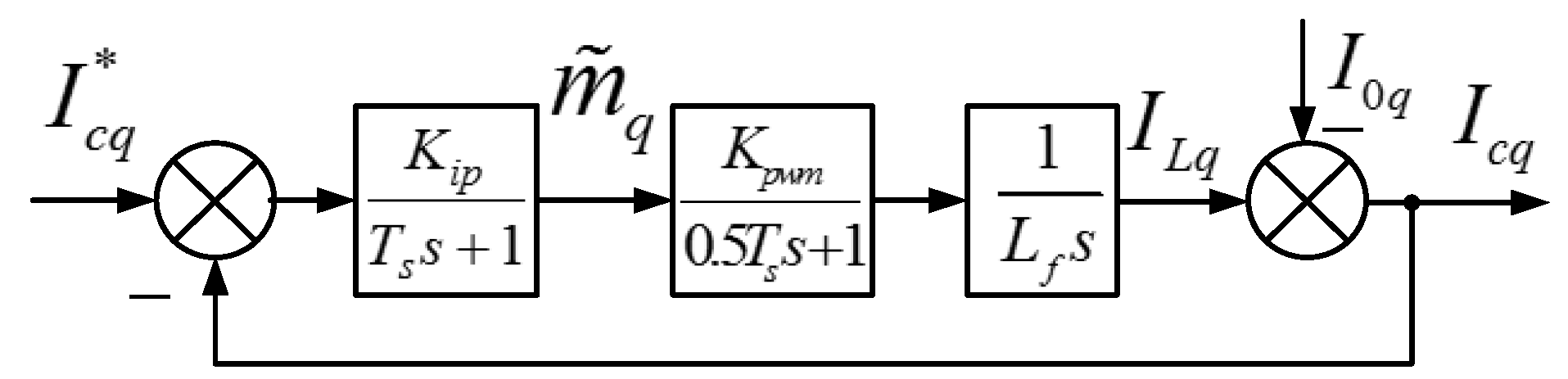
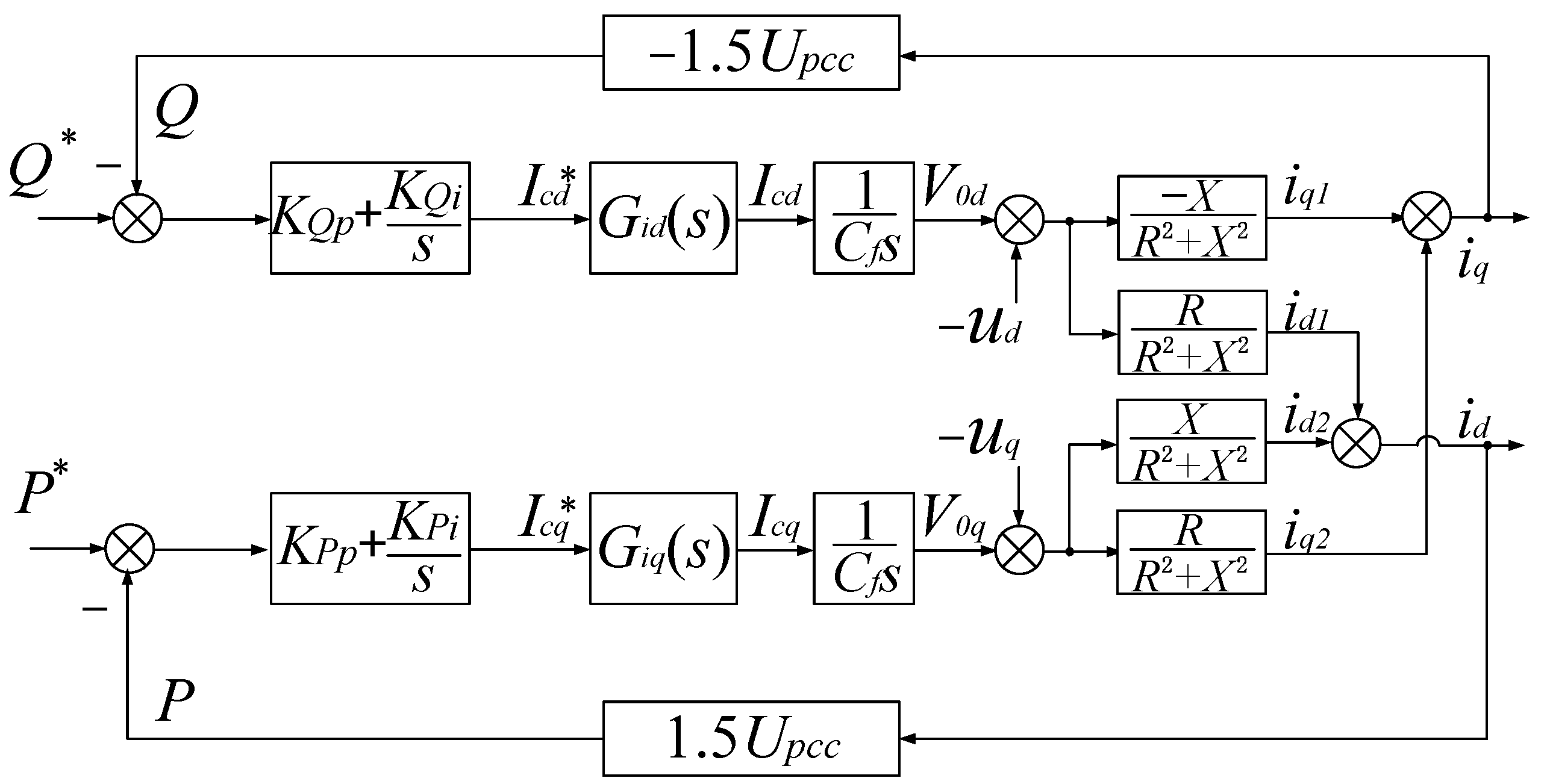
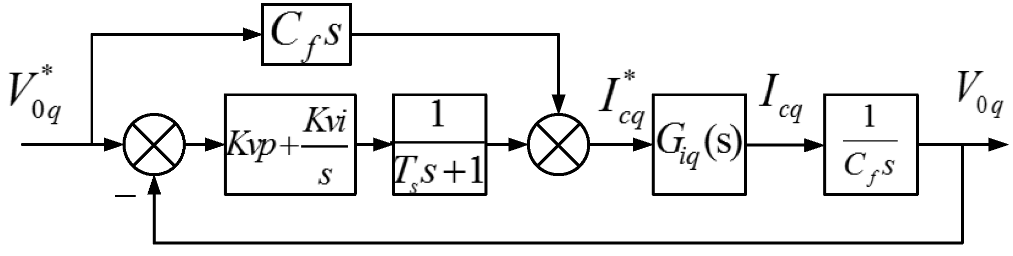
3.1. PQ Control Method

To improve the response speed and accuracy of power distribution, the PQ control method is adopted [20,21,22]. Double-loop control structure is employed: the inner loop uses current control to ensure response speed, thereby improving the operation characteristics of the system; the outer loop adopts power control [23].
The structure of inner current loop is shown in Figure 3 [24].
In Figure 3, Vcd and Vcq are the d,q axis voltage component of converters and Vod and Voq are the d,q axis voltage components of the filter; Lf is the inductance of filter; Kip and Kii are the proportional and integral parameters of the proportional-integral (PI) controller.
To satisfy the decoupling condition of the d,q axis, “virtual impedance” is introduced in low-voltage AC MG [25,26]. After decoupling, structure of the q axis is chosen to analyze because d,q share the same structure. Considering the pulse-width modulation (PWM) and the sampling process, the control diagram is shown in Figure 4.
As shown above, Ts is the time constant of sampling and its value is pretty small. 1/(Tss + 1) and 1/(0.5Tss + 1) are the delay modules of sampling and PWM, and they can approximately merge into 1/(1.5Tss + 1) [27]. Set up the switching frequency of the system as: fs = 20 kHz, Ts = 1/fs = 0.05 ms. The gain of the modulator is Kpwm = Udc/2 = 400.
Then, the open-loop transfer function is as shown
G i q 0 ( s ) = K i p K p w m ( 1.5 T s s + 1 ) L f s .
Similarly, the open-loop transfer function of the d-axis is
G i d 0 ( s ) = K i p K p w m ( 1.5 T s s + 1 ) L f s .
In order to impose that the cut-off frequency of control is 0.1 times the switching frequency, the following relations must be satisfied:
{ ω x = 2 π f s 10 20 lg | G i q 0 ( j ω x ) | = 0 ,
where ωx is the designed cut-off frequency.
If the switching frequency of the PWM modulator is 20 kHz, set up the inductor-capacitor (LC) passive filter’s inductance Lf as 1.5 mH. Kip ≈ 0.065 can be obtained. The design principles of the converter output LC passive filter is
{ 10 f n f c f s / 5 2 π f c L f = 1 / ( 2 π f c C f ) ,
where fc is the designed resonant frequency of filter, and fn is the fundamental frequency. Setting up Lf is 1.5 mH and Cf is 20 μF.
Based on the above analysis, the control structure of the PQ control method is shown in Figure 5 [28].
As shown, Kpp and Kpi are the proportional and integral parameters of the PI controller for active power, respectively; KOp and KOi are appropriate parameters for reactive power. Due to the symmetry of the two parts, it makes KPp = KQp and KPi = KQi. In addition, P*, Q* are the reference values of active and reference power, respectively. After decoupling, the open-loop transfer function is shown
{ G Q ( s ) = 1.5 U p c c ( K Q p s + K Q i ) C f X s 2 G i d ( s ) G P ( s ) = 1.5 U p c c ( K P p s + K P i ) C f X s 2 G i q ( s ) .

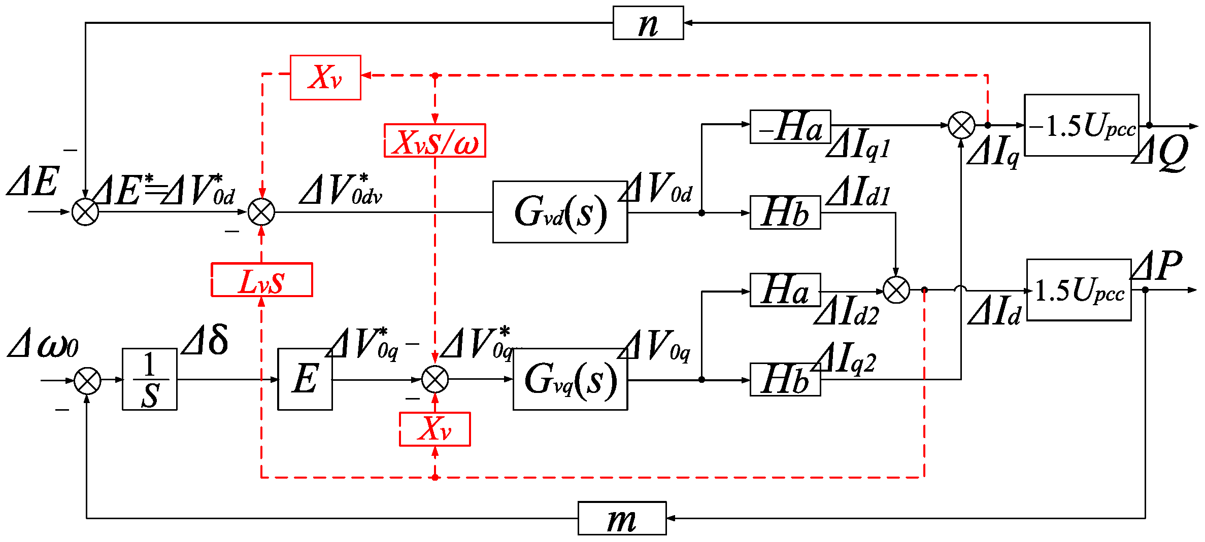
3.2. Inductive Droop Control

The DGs with droop control can independently adjust the balance of frequency and voltage and control the operation of MG as the main control micro source. Its control structure still adopts voltage-current double loop structure, where the principle of its current control loop is similar to Section 2.1. Likewise, the q-axis structure of voltage control loop after decoupling is shown in Figure 6.
The open-loop transfer function in this structure is [29]
G v q 0 ( s ) = G i q ( s ) ( K v p s + K v i ) C f ( T s s + 1 ) s 2 .
It is necessary to install an LC passive filter at the converter outlet to filter high order harmonics, which can be designed as Equation (3).
This paper adopts: fn = 50 Hz, fs = 20 kHz, fc = 1000 Hz. Considering the voltage drop on filter inductance, Lf = 1.5 mH, and Cf = 16.89 μF can be obtained. At this point, the PI parameters of outer loop must be satisfied:
20 lg | G v q 0 ( j ω x ) | = 0 .
Taking the stability and rapidity into account, Kvp = 0.1 and Kvi = 407.65 can be obtained; then, Kvi = 400.
The converter is connected to the point of common coupling (PCC). The voltage of this point is a planned constant and selected as the reference voltage, that is: Upcc < 0 = Upcc + j0, the output voltage of converter filter is: V0 < θ = V0d + jV0q. Supposing that the impedance of low-voltage MG is Rl + jXl, where Xl = ωLl, ω is the AC signal frequency, Ll is the equivalent inductance of transmission line; then, the voltage and current relation of the d and q axes are
{ V 0 d U p c c = ( R l + L l s ) I 0 d X l I 0 q V 0 q 0 = ( R l + L l s ) I 0 q + X l I 0 d .
The expression of small signal quantity of the current as shown is
{ Δ I 0 q = Δ I 0 q 1 + Δ I 0 q 2 = H a × Δ V 0 d + H b × Δ V 0 q Δ I 0 d = Δ I 0 d 1 + Δ I 0 d 2 = H b × Δ V 0 d + H a × Δ V 0 q ,
where Ha and Hb can be expressed as
H a = X l X l 2 + ( R l + L l s ) 2 ;   H b = ( R l + L l s ) X l 2 + ( R l + L l s ) 2 .
Actually, I0d and I0q are DC variables, and their differential results are negligible for Lls and much smaller than Xl.
P + jQ = Upcc(I0djI0q) is the power equation in the dq0 coordinate system, and the power small signal model can be obtained:
{ Δ Q = 1.5 U p c c ( Δ I 0 q 1 + Δ I 0 q 2 ) Δ P = 1.5 U p c c ( Δ I 0 d 1 + Δ I 0 d 2 ) .
For double loop structure, the virtual impedance is equivalent to introducing a logical inductive feedback link in essence, which corrects the reference voltage of dual-loop control and controls the output power further.
Supposing that θ is quite small, then V0q*= E*sinθE*θ, V*0dE*, where E* is the reference voltage from reactive droop loop. Furthermore, it can be considered that ΔV*0qEΔθ because changes of E* are much smaller than that of θ, where E is the reference voltage before reactive droop loop. The control structure is shown in Figure 7 [26].
After reasonable setting of virtual impedance, it is equivalent that the previous line impedance connects in series with a reactance Xv, which satisfies the following relationship Xv + Xv >> Rl, and then Rl in Ha and Hb can be neglected, that is Hb = 0, indicating the realization of decoupling in droop control.

4. Small Signal Modeling of Three-Source MG

Theoretical analysis of a three-source MG with all DGs working at the same time is performed on the basis of model built in Section 1.1. To help analyze the stability of system, the electrical quantities are expressed in steady state small signal equations [30,31], according to the relationship of voltage and current in dq0 coordinate system:
{ Δ V o d n Δ U G d = ( R n + X n ω s ) Δ i d n X n Δ i q n Δ V o q n Δ U G q = ( R n + X n ω s ) Δ i q n + X n Δ i d n .
Generally, the differential terms in Equation (11) has less influence and can be ignored. Therefore, the system model satisfies Equation (12):
{ Δ V o d 1 Δ U G d = R 1 Δ i d 1 X 1 Δ i q 1 Δ V o q 1 Δ U G q = R 1 Δ i q 1 + X 1 Δ i d 1 Δ V o d 2 Δ U G d = R 2 Δ i d 2 X 2 Δ i q 2 Δ V o q 2 Δ U G q = R 2 Δ i q 2 + X 2 Δ i d 2 Δ V o d 3 Δ U G d = R 3 Δ i d 3 X 3 Δ i q 3 Δ V o q 3 Δ U G q = R 1 Δ i q 3 + X 1 Δ i d 3 0 Δ U G d = R 4 Δ i d 4 X 4 Δ i q 4 0 Δ U G q = R 2 Δ i q 4 + X 4 Δ i d 4 Δ i d 1 + Δ i d 2 + Δ i d 3 + Δ i d 4 = 0 Δ i q 1 + Δ i q 2 + Δ i q 3 + Δ i q 4 = 0 .
Assuming that ΔVod1, ΔVoq1, ΔVod2, ΔVoq2, ΔVod3, ΔVoq3, R1, X1, R2, X2, R3, X3, R4, X4 are known, Δid1, Δiq1, Δid2, Δiq2, Δid3, Δiq3, Δid4, Δiq4 can be expressed with the above quantities by solving Equation (12), ΔUGd, ΔjUGq by Equation (13):
{ Δ U G d = J 1 Δ V o d 1 + J 2 Δ V o d 2 + J 3 Δ V o d 3 + J 4 Δ V o q 1 + J 5 Δ V o q 2 + J 6 Δ V o q 3 Δ U G q = J 7 Δ V o d 1 + J 8 Δ V o d 2 + J 9 Δ V o d 3 + J 10 Δ V o q 1 + J 11 Δ V o q 2 + J 12 Δ V o q 3 .
It is clear that X1 >> R1, X2 >> R2 [25,26] when DG1 and DG2 adopt the droop control method, and then the influence of line resistance can be ignored, that is: R1 = R2 = 0. Suppose that the load is mostly active and then: X4 = 0. Therefore, the coefficients in Equation (13) can be expressed as
{ J 1 = J 10 = [ R 3 2 R 4 2 ( X 1 X 2 + X 2 2 ) + R 4 2 X 2 X 3 ( X 1 X 2 + X 1 X 3 + X 2 X 3 ) ] / D d J 2 = J 11 = [ R 3 2 R 4 2 ( X 1 X 2 + X 1 2 ) + R 4 2 X 1 X 3 ( X 1 X 2 + X 1 X 3 + X 2 X 3 ) ] / D d J 3 = J 12 = [ R 3 R 4 X 1 2 X 2 2 + R 4 2 X 1 X 2 ( X 1 X 2 + X 1 X 3 + X 2 X 3 ) ] / D d J 4 = J 7 = [ R 4 X 1 X 2 2 ( R 3 2 + R 3 R 4 + X 3 2 ) ] / D d J 5 = J 8 = [ R 4 X 1 2 X 2 ( R 3 2 + R 3 R 4 + X 3 2 ) ] / D d J 6 = J 9 = [ R 3 R 4 2 X 1 X 2 ( X 1 + X 2 ) + R 4 X 1 2 X 2 2 X 3 ] / D d D d = R 3 2 R 4 2 ( X 1 + X 2 ) 2 + ( R 1 + R 2 ) 2 X 1 2 X 2 2 + X 1 2 X 2 2 X 3 2 + 2 R 4 2 X 1 X 2 X 3 ( X 1 + X 2 + X 3 ) + R 4 2 X 3 2 ( X 1 2 + X 3 2 ) .
After ignoring the differential terms, model of droop control is shown by Equations (13) and (14) is obtained from model of PQ control:
{ [ Δ E 1 * 3 n 1 U p c c 2 X 1 ( Δ V o d 1 Δ U G d ) ] G v d 1 ( s ) = Δ V o d 1 [ Δ ω 01 * 3 m 1 U p c c 2 X 1 ( Δ V o q 1 Δ U G q ) ] G v q 1 ( s ) = Δ V o q 1 [ Δ E 2 * 3 n 2 U p c c 2 X 2 ( Δ V o d 2 Δ U G d ) ] G v d 2 ( s ) = Δ V o d 2 [ Δ ω 02 * 3 m 2 U p c c 2 X 2 ( Δ V o q 2 Δ U G q ) ] G v q 2 ( s ) = Δ V o q 2 ,
{ G Q ( s ) { Δ Q 3 * + 1.5 U p c c [ X 3 M + R 3 N ] } = Δ V o d 3 G P ( s ) { Δ P 3 * 1.5 U p c c [ R 3 M + X 3 N ] } = Δ V o d 3 M = ( Δ V o d 3 Δ U G d ) X 3 2 + R 3 2 N = ( Δ V o q 3 Δ U G q ) X 3 2 + R 3 2 .
To simplify the equations, setting up H1 = 1.5n1Upcc/X1, H2 = 1.5m1Upcc/X1, H3 = 1.5n2Upcc/X2, H4 = 1.5m2Upcc/X2, H5 = 1.5UpccX3/( X 3 2 + R 3 2 ), H6 = 1.5UpccR3/( X 3 2 + R 3 2 ), by solving simultaneously Equations (15) and (16), Equation (17) is obtained.
{ [ Δ E 1 * H 1 ( Δ V o d 1 Δ U G d ) ] G v d 1 ( s ) = Δ V o d 1 [ Δ ω 01 * H 2 ( Δ V o q 1 Δ U G q ) ] G v q 1 ( s ) = Δ V o q 1 [ Δ E 2 * H 3 ( Δ V o d 2 Δ U G d ) ] G v d 2 ( s ) = Δ V o d 2 [ Δ ω 02 * H 4 ( Δ V o q 2 Δ U G q ) ] G v q 2 ( s ) = Δ V o q 2 G Q ( s ) [ Δ Q 3 * H 5 ( Δ V o d 3 Δ U G d ) +    H 6 ( Δ V o q 3 Δ U G q ) ] = Δ V o d 3 G P ( s ) [ Δ P 3 * H 6 ( Δ V o d 3 Δ U G d ) +    H 5 ( Δ V o q 3 Δ U G q ) ] = Δ V o d 3 ,
where Δ E 1 * and Δω0i* are the reference voltage and reference frequency of DGi (I = 1, 2), which adopts droop control.
By solving Equations (13) and (17), Equation (18) can be obtained:
[ Δ U G d Δ U G q ] T = H G 2 × 6 [ Δ E 1 * Δ ω 01 * Δ E 2 * Δ ω 02 * Δ Q 3 * Δ P 3 * ] T .
On the premise of guaranteeing the stability of the inner loop, Gid(s) = Giq(s) = 1 is reasonable [21,32]; therefore, Gvd(s) = Gvq(s) = 1. In addition, HG is a matrix of 2 × 6, whose simplified one is shown in Equation (19):
[ Δ U G d Δ U G q ] = [ C 1 ( s ) D ( s ) C 2 ( s ) D ( s ) C 3 ( s ) D ( s ) C 4 ( s ) D ( s ) C 5 ( s ) D ( s ) C 6 ( s ) D ( s ) F 1 ( s ) D ( s ) F 2 ( s ) D ( s ) F 3 ( s ) D ( s ) F 4 ( s ) D ( s ) F 5 ( s ) D ( s ) F 6 ( s ) D ( s ) ] × [ Δ E 1 * Δ ω 01 * Δ E 2 * Δ ω 02 * Δ Q 3 * Δ P 3 * ] T .
As shown above, Equation (19) is the small-signal control model of the islanded MG, elements of whose coefficient matrix share the same denominator named D(s). By analyzing the characteristic equation D(s) = 0, the stability of the system can be determined.

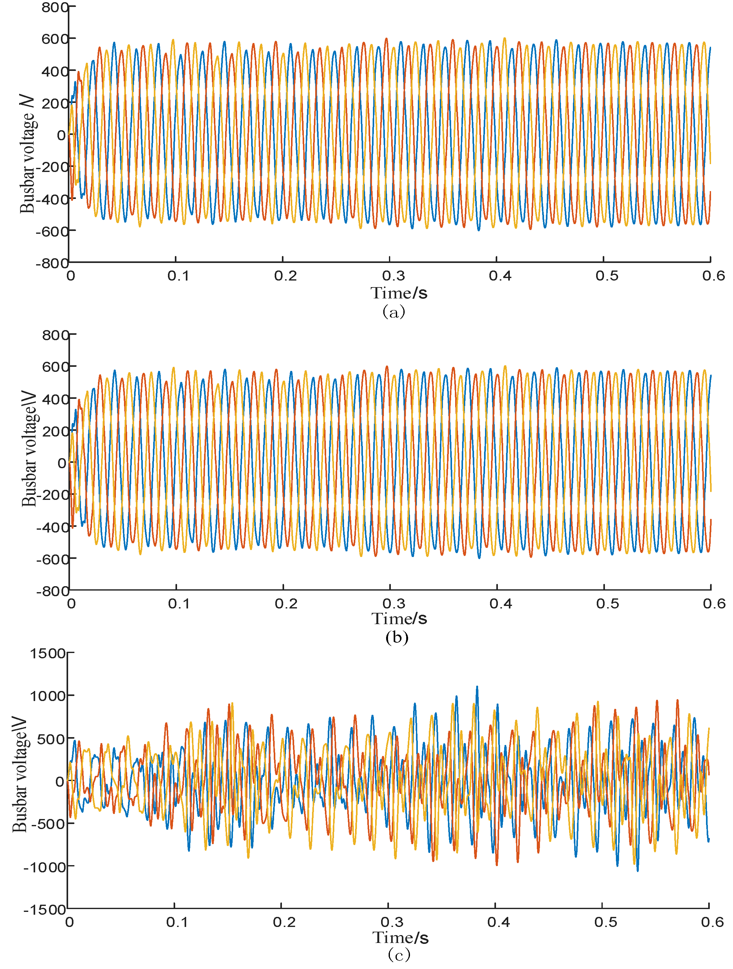
5. Simulation and Stability Analysis

5.1. Parameter Setting and Calculation

Based on Figure 1, DG1 and DG2 should satisfy: P1 = 30,000 − (f − 50)/m1, P2 = 30,000 − (f − 50)/m2, Q1 = 5000 − (E1 − 311)/n1, Q2 = 5000 − (E2 − 311)/n2.
Using the parameters in Appendix A, H1H6 can be obtained: H1 = 466.5n1, H2 = 466.5m1, H3 = 466.5n2, H4 = 466.5m2, H5 = 208.6 and H6 = 417.2.

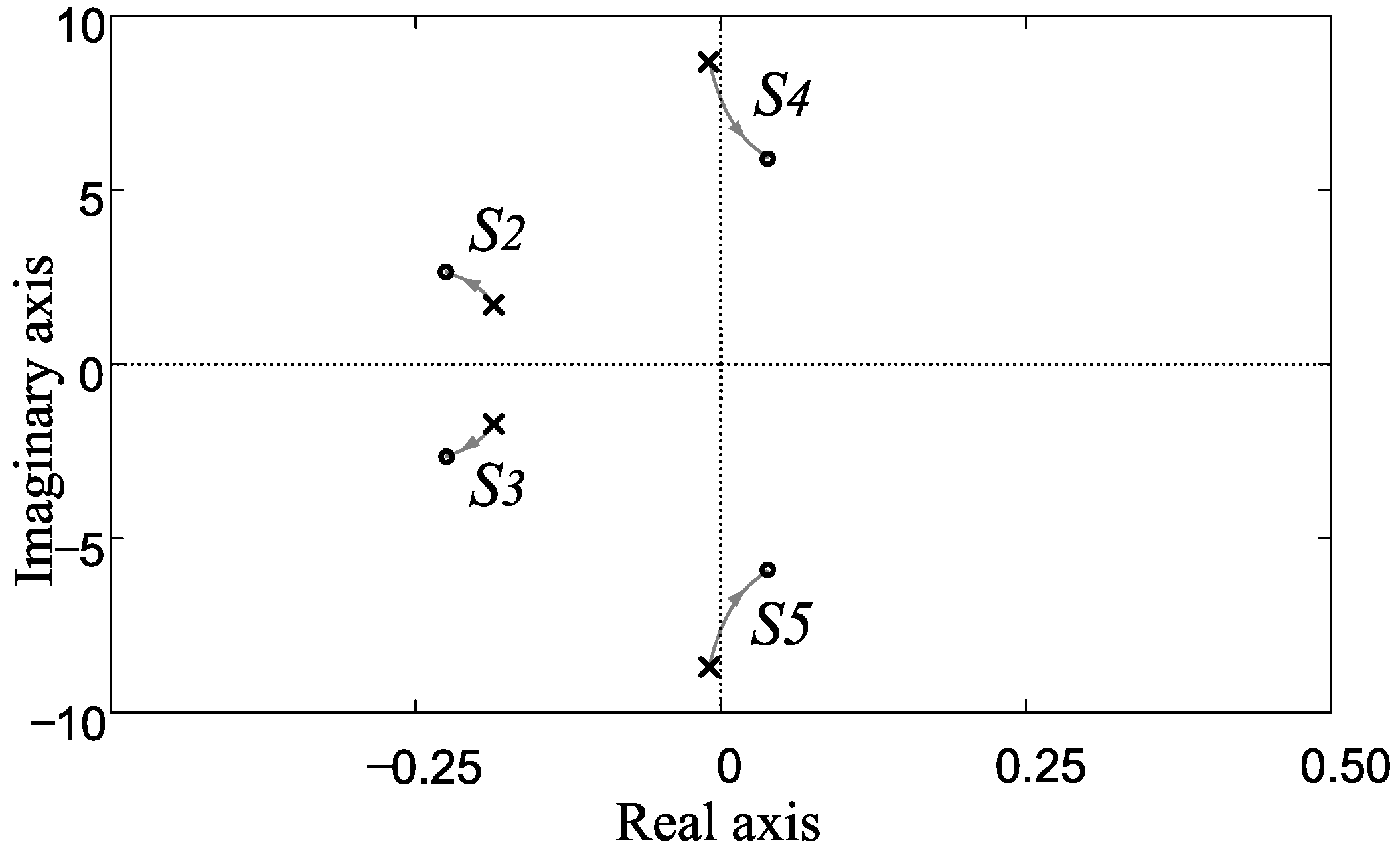
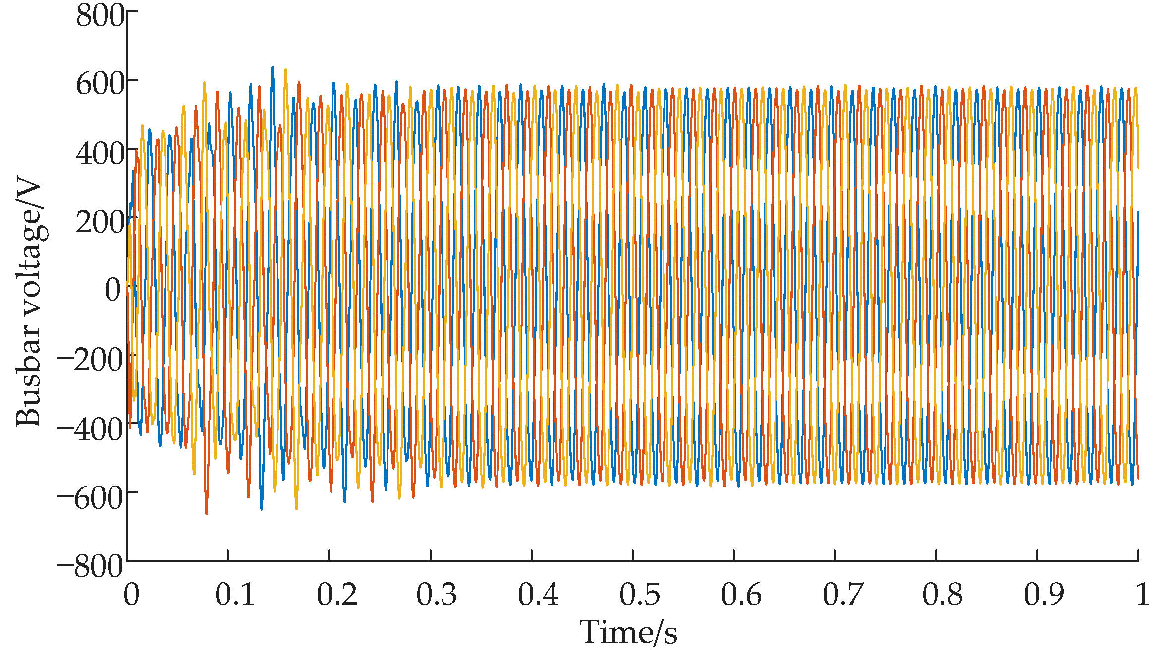
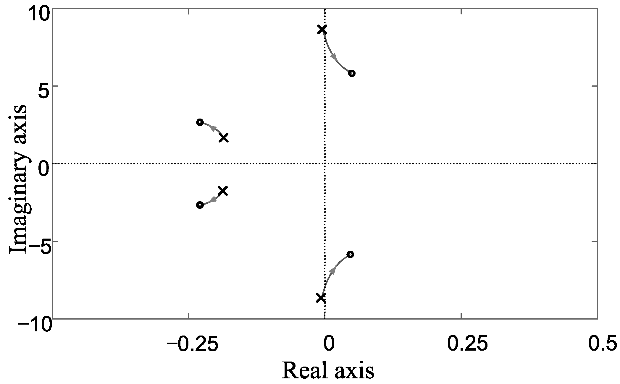
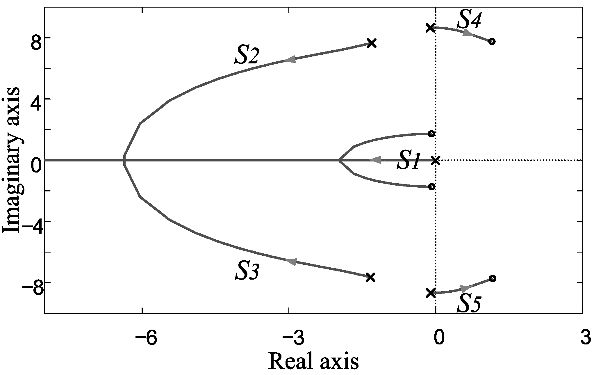
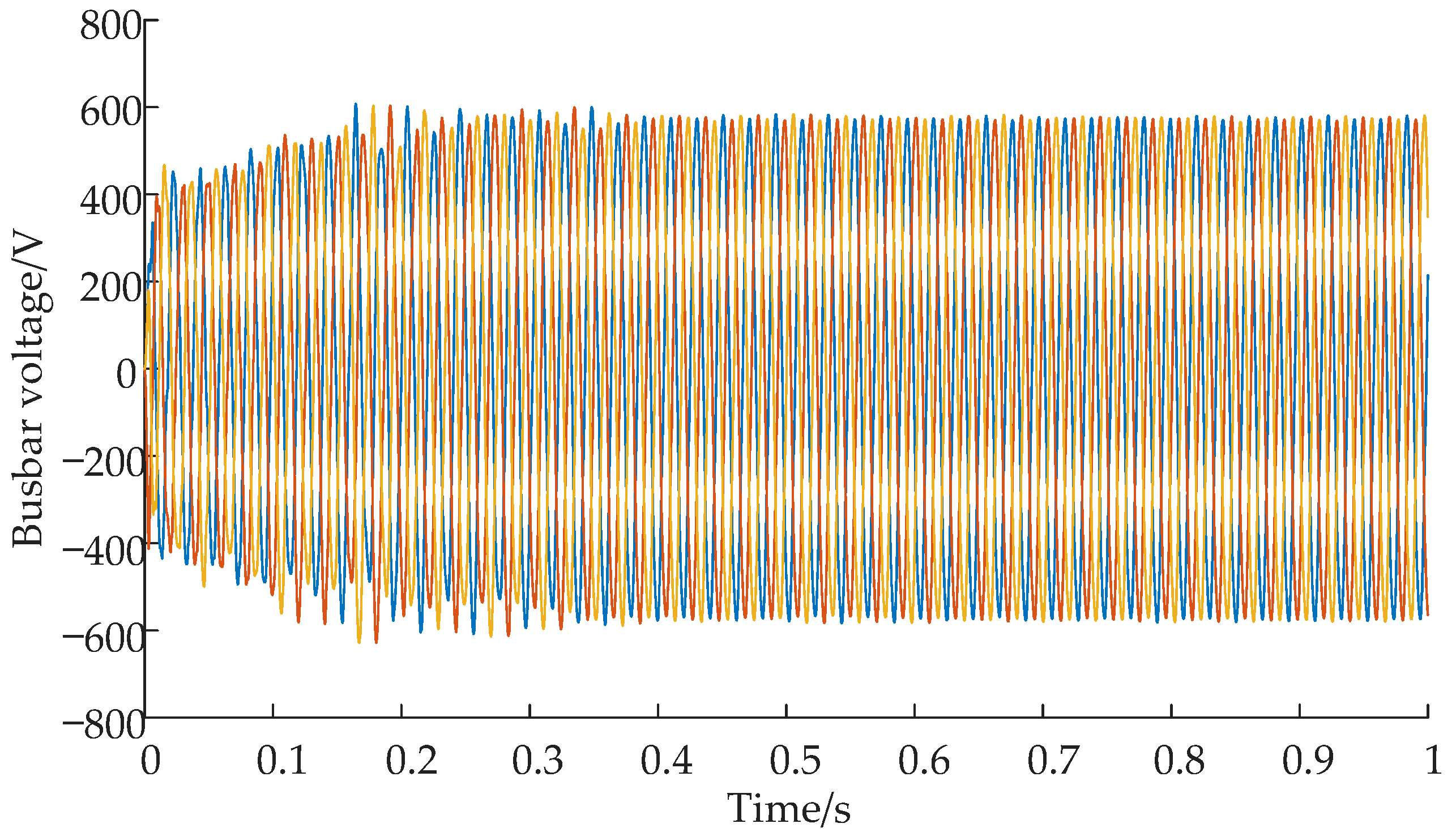
5.2. Influence of Active Droop Coefficient m1 and m2 on Stability

To explore the impact of single variable m1 on system stability, a priority assignment is first implemented: n1 = n2 = 0.001 V/var, KPp = KQp = 0.0005, KPi = KQi = 0.5.
(1) When m2 = 5 × 10⁻⁵ Hz/W, the characteristic equation D(s) = 0 is
( m 1 + 0.00242 ) s 5 + ( 234 m 1 + 0.542 ) s 4 + ( 125 m 1 + 0.392 ) s 3 + ( 9860 m 1 + 42.3 ) s 2 + ( 3790 m 1 + 15.7 ) s + ( 58,000 m 1 + 122 ) = 0 .
The root locus equation as Equation (20) whose gain is m1 can be acquired by processing Equation (21):
m 1 W 1 ( s ) + 1 = 0 ,
where W1(s) and the similar expressions hereafter in this paper can be found in Appendix B.
The root locus of D(s) when m1 varies from 0 to +∞ is shown in Figure 8.
There are five branches, S1 starts from (−233.8x, 0) to (−225.3, 0) and always stays in left half-plane and far away from the imaginary axis, so it is not shown in the picture; S2 and S3 locate in left half-plane and have no impact on stability; S4 and S5 move towards the positive direction with the change of m1, leading to the decline in stability, they finally cross the imaginary axis (m1 = 3.2 × 10⁻⁵) and enter the right half-plane indicating that the system is no longer stable. Therefore, the proper range of m1 to ensure system stability is [0, 3.2 × 10⁻⁵) in this condition.
Theoretically, the smaller m1 is, the weaker the impact of change in DG1’s output power on system’s frequency is, especially when m1 = 0, DG1 works in constant frequency control mode and has the strongest stability. At this point, DG1 has theoretically infinite power supply, which owns the absolute frequency stability and peak regulating ability. However, this assumption is not consistent with the energy attributes of MG. That is, MG’s output power is limited and relies on other MGs’ cooperation, so m1 cannot be too small. On the other hand, a large value of m1 also results in the fast oscillation of system frequency under small power fluctuation, which is harmful to system stability and this situation is shown in Figure 8 when m1 > 3.2 × 10⁻⁵.
When m1 = 2.5 × 10⁻⁵ Hz/W and m2 = 5 × 10⁻⁵ Hz/W, the bus voltage waveform is shown in Figure 9. Because 2.5 × 10⁻⁵ ∈ [0, 3.2 × 10⁻⁵) and the bus voltage is stable, it means that the m1 in this range ensures microgrid stable operation, which can verify the correctness of above analysis.
(2) When m2 = 10 × 10−5 Hz/W, the root locus equation whose gain is m1 is
m 1 W 2 ( s ) + 1 = 0 .
The root locus of D(s) when m1 varies from 0 to +∞ is shown in Figure 10.
The locus is so similar to Figure 8 that it won’t be described again. The proper range of m1 is [0, 2.9 × 10⁻⁵), and system stability declines with the increase of m1.
When m1 = 2 × 10⁻⁵ Hz/W and m2 = 10 × 10−5 Hz/W, the bus voltage waveform is shown in Figure 11. The waveform is similar to Figure 9, without more detailed analysis.
(3) When m2 = 2.5 × 10⁻⁵ Hz/W, the root locus equation whose gain is m1 is
m 1 W 3 ( s ) + 1 = 0 .
The root locus of D(s) when m1 varies from 0 to +∞ is shown in Figure 12.
The locus is so similar to Figure 8 that it won’t be described again. The proper range of m1 is [0, 7.21 × 10⁻⁵), and system stability declines with the increase of m1.
When m1 = 5 × 10⁻⁵ Hz/W and m2 = 2.5 × 10⁻⁵ Hz/W, the bus voltage waveform is shown in Figure 13. The waveform is similar to Figure 9, without more detailed analysis.
In summary, the comparison of range for m1 when m2 is different is shown in Table 1. In Table 1, m1 is less than 2.9 × 10⁻⁵ when m2 is 10 × 10−5. It is the reason why bus voltage is unstable in Section 1.2. The allowable range of m1 narrows with the increase of m2. From the perspective of system stability, the active droop coefficients of two DGs are supposed to be coordinated and restricted in a lower range so that the unit power loss won’t cause large change in frequency and system frequency collapse.

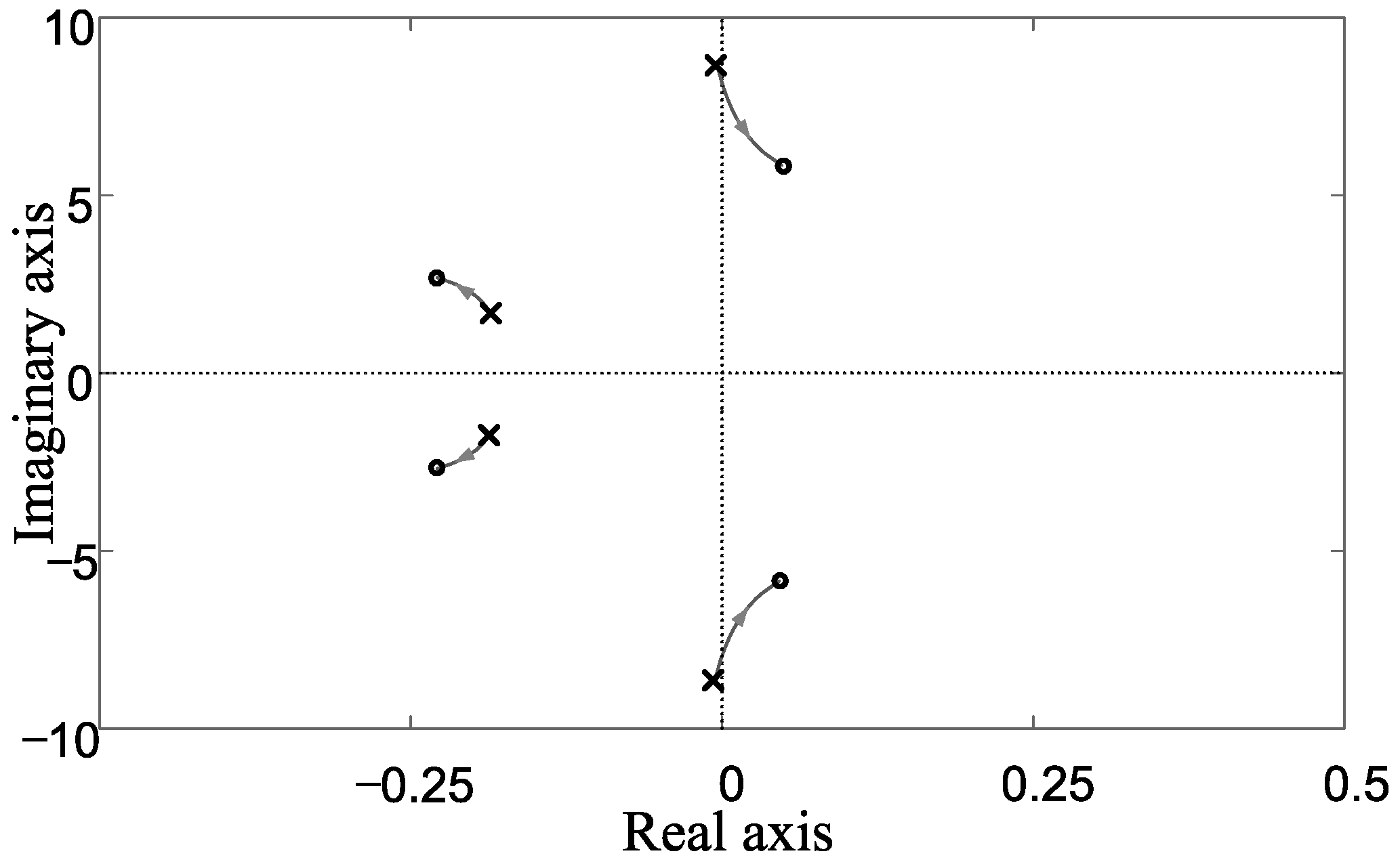
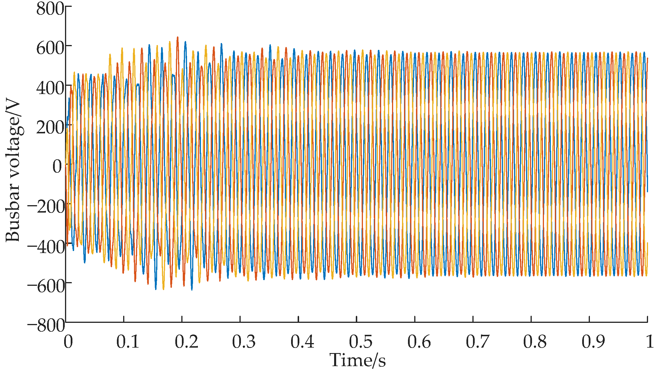
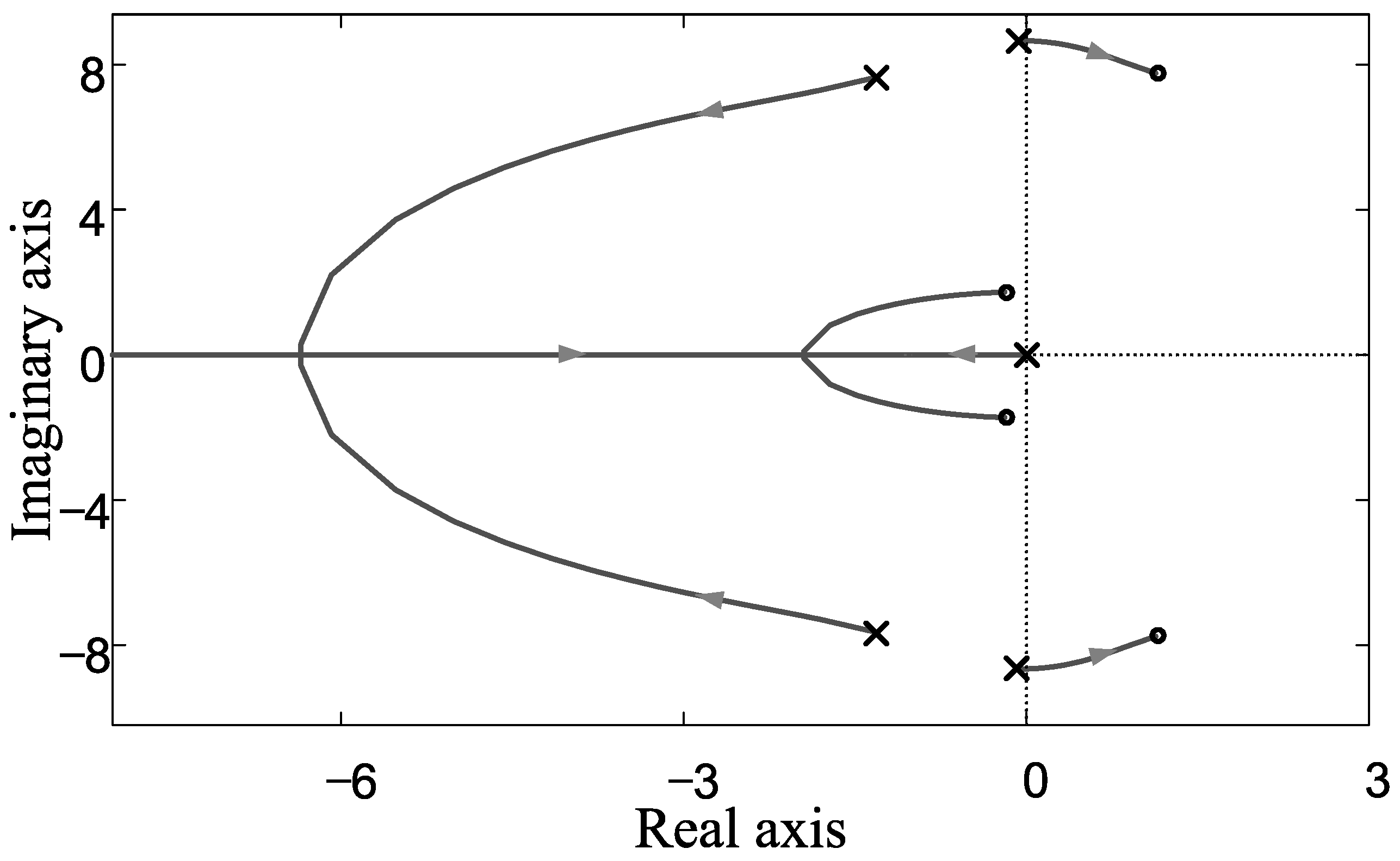
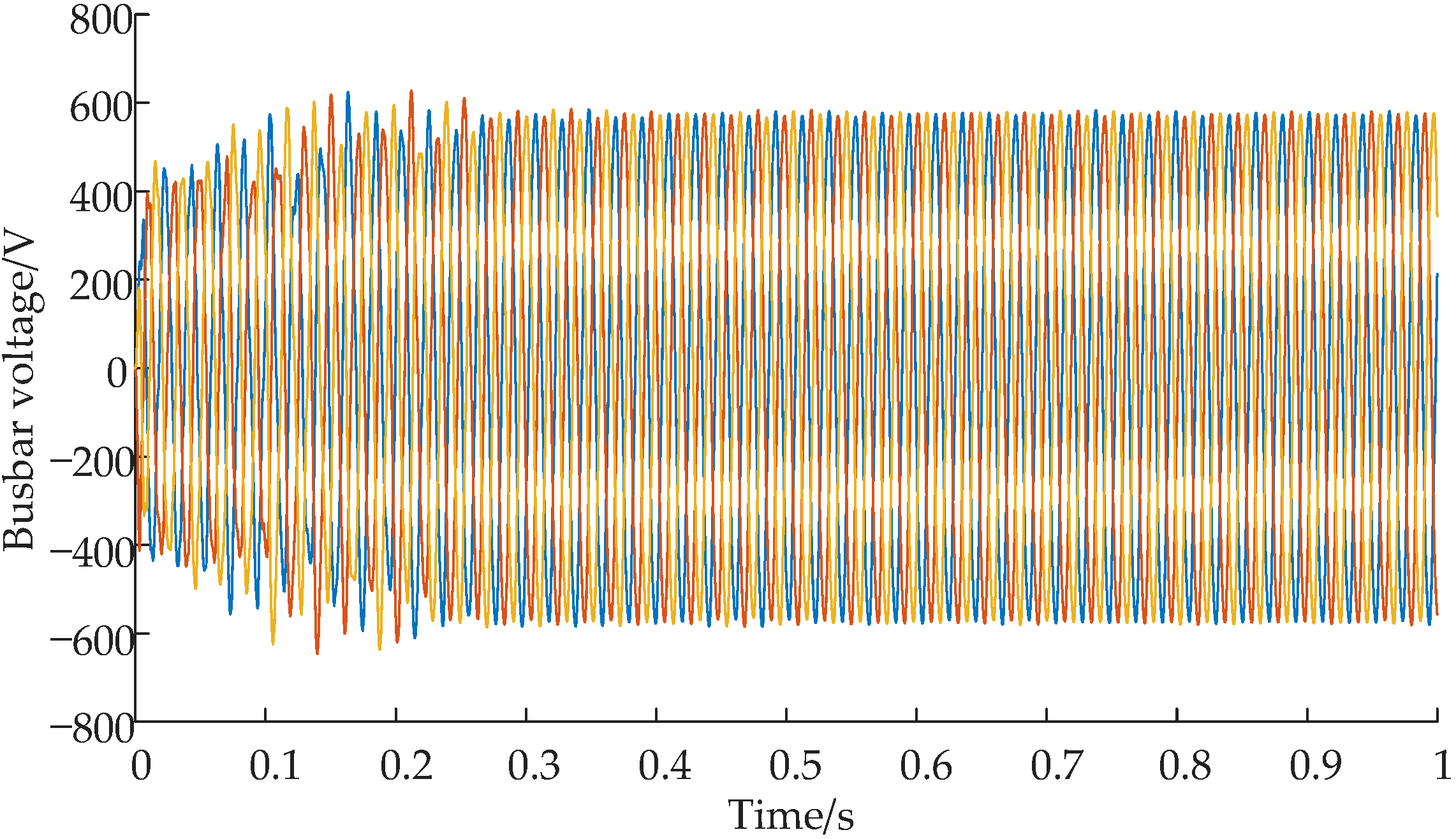
5.3. Influence of Reactive Droop Coefficient n1 and n2 on Stability

To explore the impact of single variable n1 on system stability, a priority assignment is first implemented: m1 = m2 = 2.5 × 10⁻⁵ Hz/W, KPp = KQp = 0.0005, KPi = KQi = 0.5.
(1) When n2 = 0.002 V/var, the root locus of the equation D(s) = 0 whose gain is n1 is
n 1 W 4 ( s ) + 1 = 0 .
The root locus when n1 varies from 0 to +∞ is shown in Figure 14.
There are six branches, S1 first moves towards left and then turns right and always stays in the left half-plane, indicating that the system stability first enhances and then degrades; S2 and S3 are located in the left half-plane and have no impact on stability; S4 and S5 move towards the positive direction with the change of n1, leading to the decline in stability, they finally cross the imaginary axis (n1 = 0.00147) and enter the right half-plane indicating that the system is no longer stable. Therefore, the proper range of n1 to ensure system stability is [0, 0.00147) in this condition.
Theoretically, the smaller n1 is, the weaker the impact of change in DG1’s output reactive power on system’s voltage is. Especially when n1 = 0, DG1 works in constant voltage control mode and has the strongest stability. At this point, DG1 has theoretically infinite reactive power supply, which owns the absolute voltage stability and reactive power compensation ability. However, this assumption is not consistent with the energy attributes of MG. That is, MG’s output reactive power is limited and relies on other MGs’ cooperation, so n1 cannot be too small. On the other hand, a large value of n1 also results in voltage collapse under small reactive power fluctuation, and this instable situation is shown in picture when n1 > 0.00147.
When n1 = 0.001 V/var and n2 = 0.002 V/var, the bus voltage waveform is shown in Figure 15. Because 0.001 ∈ [0, 0.00147) and the bus voltage is stable, it means that the n1 in this range ensures microgrid stable operation, which can verify the correctness of the above analysis.
(2) When n2 = 0.001 V/var, the root locus equation is
n 1 W 5 ( s ) + 1 = 0 .
The root locus of D(s) when n1 varies from 0 to +∞ is shown in Figure 16.
Because this locus is similar to Figure 14, it won’t be described again. The proper range of n1 is [0, 0.00169), and system stability declines with the increase of n1.
When n1 = 0.001 V/var and n2 = 0.001 V/var, the bus voltage waveform is shown in Figure 17. The waveform is similar to Figure 15, without more detailed analysis.
(3) When n2 = 0.004 V/var, the root locus equation is
n 1 W 6 ( s ) + 1 = 0 .
The root locus of D(s) when n1 varies from 0 to +∞ is shown in Figure 18.
Because this locus is similar to Figure 14, it won’t be described again. The proper range of n1 is [0, 0.00133), and system stability declines with the increase of n1.
When n1 = 0.001 V/var and n2 = 0.004 V/var, the bus voltage waveform is shown in Figure 19. The waveform is similar to Figure 15, without more detailed analysis.
In summary, the comparison of range of n1 when n2 is different is shown in Table 2. The allowable range of n1 narrows with the increase of n2. From the perspective of system stability, the reactive droop coefficients of two DGs are supposed to be coordinated because it is restricted in such a low value range that the unit reactive power loss won’t cause large change in voltage—thus avoiding the vicious cycle: “change in voltage-reactive power loss-enlargement change in voltage—larger reactive power loss”.

6. Conclusions

In this paper, research on influence of the wide application of electronic devices on system stability is done by a three-source MG with a multiple master-slave control method.
Different from the traditional master–slave control model, this paper established a model where several master controllers coordinate and control the system in islanded mode. Then, the “virtual impedance” was introduced to satisfy the decoupling condition and the small-signal decoupling control model, which contains two main control sources and subordinate one, was also developed on the basis of theory. Finally, the interaction between various DGs with droop control from the perspective of control parameters was explored with the aid of the root locus method. The results show that the value range of the droop coefficient for the two main DGs has mutual influence and the coordinated allocation of parameters also affects the stability of microgrid operation. This research could serve as a reference for parameter setting and contributed to study on stability of multi-source MG.

Author Contributions

All of the authors contributed to this work. H.L. and P.L. provided important comments on the modeling and designed the experiments; Y.D. and C.Z. performed the experiments and analyzed the data; Y.D. and Y.H. wrote the whole paper.

Funding

This research was funded by the National Natural Science Foundation of China (No. 51577068) and the National High Technology Research and Development Program of China (No. 2015AA050101). And the APC was funded by North China Electric Power University.

Acknowledgments

The authors gratefully acknowledge the support from the National Natural Science Foundation of China (No. 51577068) and the National High Technology Research and Development Program of China (No. 2015AA050101).

Conflicts of Interest

The authors declare no conflict of interest.

Appendix A

Table A1. System basic parameter value.
Meaning of ParameterSymbol of ParameterValue of Parameter
Voltage Level/VE*311
Reference value of active power/kWP3*10
Reference value of reactive power/kVarQ3*−10
System switching frequency/kHzfs20
System sampling period/msTs0.05
Filter inductors/mHLf1 = Lf2 = Lf31.5
Filter capacitors/μFCf1 = Cf2 = Cf320
Line resistance of DG1 and DG2/ΩR1, R20
Line resistance of DG3/ΩR30.2
Load resistance/ΩR43
Line inductance of DG1 and DG2/ΩX1 = X21.0
Line inductance of DG3/ΩX30.1
Load inductance/ΩX40
Proportional coefficient of voltage loopKvp0.1
Integral coefficient of voltage loopKvi400
Proportional coefficient of current loopKip0.065

Appendix B

The expressions of coefficients W1(s)–W6(s) in Equations (21)–(26) are shown in (A1)–(A6).
W 1 ( s ) = 412.78 s 5 + 96,596 s 4 + 51,663 s 3 + 4,069,653 s 2 + 1,562,487 s + 23,925,000 s 5 + 223.78 s 4 + 161.64 s 3 + 17,462 s 2 + 6492 s + 50,574 ,
W 2 ( s ) = 413.2 s 5 + 96,818 s 4 + 51,322 s 3 + 3,997,107 s 2 + 1,536,776 s + 24,028,925 s 5 + 224.3 s 4 + 161.2 s 3 + 17,340 s 2 + 6450 s + 50,785 ,
W 3 ( s ) = 412.7 s 5 + 96,558 s 4 + 51,863 s 3 + 4,110,238 s 2 + 1,576,956 s + 23,890,375 s 5 + 223.67 s 4 + 162 s 3 + 17,538 s 2 + 6519 s + 50,501 ,
W 4 ( s ) = 128,449 s 5 + 32,460,140 s 4 + 17,352,828 s 3 + 2,532,328,040 s 2 + 490,885,015 s + 7,337,660,287 s 6 + 257.04 s 5 + 173.83 s 4 + 29,655.7 s 3 + 8295 s 2 + 952,419 s ,
W 5 ( s ) = 128,449 s 5 + 16,237,480 s 4 + 16,087,143 s 3 + 1,266,640,229 s 2 + 483,547,355 s + 3,668,830,143 s 6 + 128.6 s 5 + 159 s 4 + 14,834 s 3 + 7342 s 2 + 476,209 s ,
W 6 ( s ) = 128,449 s 5 + 64,905,460 s 4 + 19,884,196 s 3 + 5,063,703,661 s 2 + 505,560,336 s + 14,675,320,574 s 6 + 513.9 s 5 + 203.5 s 4 + 59,299 s 3 + 10,200 s 2 + 1,904,839 s .

References

  1. Marzband, M.; Javadi, M.; Pourmousavi, S.A.; Lightbody, G. An advanced retail electricity market for active distribution systems and home microgrid interoperability based on game theory. Electr. Power Syst. Res. 2018, 157, 187–199. [Google Scholar] [CrossRef]
  2. Chendan, L.; Savaghebi, M.; Guerrero, J.M.; Coelho, E.A.; Vasquez, J.C. Operation cost minimization of droop-controlled AC microgrids using multiagent-based distributed control. Energies 2016, 9, 717. [Google Scholar] [CrossRef]
  3. Amoateng, D.O.; Hosani, M.A.; Moursi, M.S.E.; Turitsyn, K.; Kirtley, J.L. Adaptive voltage and frequency control of islanded multi-microgrids. IEEE Trans. Power Syst. 2017, 33, 4454–4465. [Google Scholar] [CrossRef]
  4. Kosari, M.; Hosseinian, S.H. Decentralized reactive power sharing and frequency restoration in islanded microgrid. IEEE Trans. Power Syst. 2017, 32, 2901–2912. [Google Scholar] [CrossRef]
  5. Divshali, P.H.; Hosseinian, S.H.; Abedi, M. A novel multi-stage fuel cost minimization in a VSC-based microgrid considering stability, frequency, and voltage constraints. IEEE Trans. Power Syst. 2013, 28, 931–939. [Google Scholar] [CrossRef]
  6. Bonfiglio, A.; Brignone, M.; Invernizzi, M.; Labella, A.; Mestriner, D.; Procopio, R. A simplified microgrid model for the validation of islanded control logics. Energies 2017, 10, 1141. [Google Scholar] [CrossRef]
  7. Guo, Q.; Cai, H.; Wang, Y.; Chen, W. Distributed secondary voltage control of islanded microgrids with event-triggered scheme. J. Power Electron. 2017, 17, 1650–1657. [Google Scholar]
  8. Farrokhabadi, M.; Cañizares, C.A.; Bhattacharya, K. Frequency control in isolated/islanded microgrids through voltage regulation. IEEE Trans. Smart Grid 2017, 8, 1185–1194. [Google Scholar] [CrossRef]
  9. Serban, I. A control strategy for microgrids: Seamless transfer based on a leading inverter with supercapacitor energy storage system. Appl. Energy 2018, 221, 490–507. [Google Scholar] [CrossRef]
  10. Lin, P.; Wang, P.; Xiao, J.; Wang, J.; Jin, C.; Tang, Y. An integral droop for transient power allocation and output impedance shaping of hybrid energy storage system in DC microgrid. IEEE Trans. Power Electron. 2017, 33, 6262–6277. [Google Scholar] [CrossRef]
  11. Etemadi, A.H.; Davison, E.J.; Iravani, R. A generalized decentralized robust control of islanded microgrids. IEEE Trans. Power Syst. 2014, 29, 3102–3113. [Google Scholar] [CrossRef]
  12. Pogaku, N.; Prodanovic, M.; Green, T.C. Modeling, analysis and testing of autonomous operation of an inverter-based microgrid. IEEE Trans. Power Electron. 2007, 22, 613–625. [Google Scholar] [CrossRef]
  13. Herrera, L.; Inoa, E.; Guo, F.; Wang, J.; Tang, H. Small-signal modeling and networked control of a PHEV charging facility. IEEE Trans. Ind. Appl. 2014, 50, 1121–1130. [Google Scholar] [CrossRef]
  14. Zhu, M.; Li, H.; Li, X. Improved state-space model and analysis of islanding inverter-based microgrid. In Proceedings of the 2013 IEEE International Symposium on Industrial Electronics, Taipei, Taiwan, 28–31 May 2013; pp. 1–5. [Google Scholar]
  15. Makrygiorgou, D.I.; Alexandridis, A.T. Distributed stabilizing modular control for stand-alone microgrids. Appl. Energy 2018, 210, 925–935. [Google Scholar] [CrossRef]
  16. Wu, T.; Liu, Z.; Liu, J.; Liu, B.; Wang, S. Modeling and stability analysis of the small-AC-signal droop based secondary control for islanded microgrids. In Proceedings of the 2016 IEEE Energy Conversion Congress and Exposition (ECCE), Milwaukee, WI, USA, 18–22 September 2016. [Google Scholar]
  17. Cao, W.; Ma, Y.; Yang, L.; Wang, F.; Tolbert, L.M. D-Q impedance based stability analysis and parameter design of three-phase inverter-based ac power systems. IEEE Trans. Ind. Electron. 2017, 64, 6017–6028. [Google Scholar] [CrossRef]
  18. Yu, Z.; Ai, Q.; He, X.; Piao, L. Adaptive droop control for microgrids based on the synergetic control of multi-agent systems. Energies 2016, 9, 1057. [Google Scholar] [CrossRef]
  19. Ghalebani, P.; Niasati, M. A distributed control strategy based on droop control and low-bandwidth communication in DC microgrids with increased accuracy of load sharing. Sustain. Cities Soc. 2018, 40, 155–164. [Google Scholar] [CrossRef]
  20. Khayamy, M.; Ojo, O. A power regulation and droop mode control method for a stand-alone load fed from a PV-current solurce inverter. Int. J. Emerg. Electr. Power Syst. 2015, 16, 83–91. [Google Scholar]
  21. Shuai, Z.; Shen, C.; Yin, X.; Liu, X.; Shen, Z.J. Fault analysis of inverter-interfaced distributed generators with different control schemes. IEEE Trans. Power Deliv. 2017, 33, 1223–1235. [Google Scholar] [CrossRef]
  22. Meng, X.; Liu, Z.; Liu, J.; Wu, T.; Wang, S.; Liu, B. A seamless transfer strategy based on special master and slave DGs. In Proceedings of the 2017 IEEE Future Energy Electronics Conference and Ecce Asia, Kaohsiung, Taiwan, 3–7 June 2017. [Google Scholar]
  23. Chen, H.; Xu, Z.; Zang, F. Nonlinear control for VSC based HVDC system. In Proceedings of the 2006 IEEE Power Engineering Society General Meeting, Montreal, QC, Canada, 18–22 June 2006. [Google Scholar]
  24. Lang, H.; Yue, D.; Cao, D. Research on VSC-HVDC double closed loop controller based on variable universe fuzzy PID control. In Proceedings of the 2017 IEEE China International Electrical and Energy Conference, Beijing, China, 25–27 October 2017. [Google Scholar]
  25. Dou, C.; Zhang, Z.; Yue, D.; Song, M. Improved droop control based on virtual impedance and virtual power source in low-voltage microgrid. Iet Gener. Transm. Distrib. 2017, 11, 1046–1054. [Google Scholar] [CrossRef]
  26. Wu, X.; Shen, C.; Iravani, R. Feasible range and optimal value of the virtual impedance for droop-based control of microgrids. IEEE Trans. Smart Grid 2017, 8, 1242–1251. [Google Scholar] [CrossRef]
  27. Ramos-Fuentes, G.A.; Melo-Lagos, I.D.; Regino-Ubarnes, F.J. Odd harmonic high order repetitive control of single-phase PWM rectifiers: Varying frequency operation. Techno Lógicas 2016, 19, 63–76. [Google Scholar]
  28. Tripathi, R.N.; Singh, A.; Hanamoto, T. Design and control of LCL filter interfaced grid connected solar photovoltaic (SPV) system using power balance theory. Int. J. Electr. Power Energy Syst. 2015, 69, 264–272. [Google Scholar] [CrossRef]
  29. Shuai, Z.; Sun, Y.; Shen, Z.J.; Tian, W.; Tu, C.; Li, Y.; Yin, X. Microgrid stability: Classification and a review. Renew. Sustain. Energy Rev. 2016, 58, 167–179. [Google Scholar] [CrossRef]
  30. Coelho, E.A.A.; Cortizo, P.C.; Garcia, P.F.D. Small-signal stability for parallel-connected inverters in stand-alone AC supply systems. IEEE Trans. Ind. Appl. 2002, 38, 533–542. [Google Scholar] [CrossRef]
  31. Rasheduzzaman, M.; Mueller, J.A.; Kimball, J.W. An accurate small-signal model of inverter-dominated islanded microgrids using dq reference frame. IEEE J. Emerg. Sel. Top. Power Electron. 2017, 2, 1070–1080. [Google Scholar] [CrossRef]
  32. Ellabban, O.; Mierlo, J.V.; Lataire, P. A DSP-based dual-loop peak DC-link voltage control strategy of the Z-source inverter. IEEE Trans. Power Electron. 2012, 27, 4088–4097. [Google Scholar] [CrossRef]
Figure 1. System model of microgrid (MG) with multiple master–slave control method.
Energies 11 02223 g001
Figure 2. Waveforms of bus voltage under different working conditions in case of (a) DG1 and DG3 running; (b) DG2 and DG3 running; (c) DG1, DG2 and DG3 running together.
Energies 11 02223 g002
Figure 3. Structure of inner current loop.
Energies 11 02223 g003
Figure 4. Control structure diagram of the inner current loop.
Energies 11 02223 g004
Figure 5. Block diagram for PQ (real and reactive power) control.
Energies 11 02223 g005
Figure 6. Structure diagram of voltage loop control.
Energies 11 02223 g006
Figure 7. Droop control structure diagram in low-voltage MG.
Energies 11 02223 g007
Figure 8. The root locus of D(s) following m1 changes when m2 = 5 × 10⁻⁵ Hz/W.
Energies 11 02223 g008
Figure 9. The bus voltage waveform when m1 = 2.5 × 10⁻⁵ Hz/W and m2 = 5 × 10⁻⁵ Hz/W.
Energies 11 02223 g009
Figure 10. The root locus of D(s) following m1 changes when m2 = 10 × 10−5 Hz/W.
Energies 11 02223 g010
Figure 11. The bus voltage waveform when m1 = 2 × 10⁻⁵ Hz/W and m2 = 10 × 10−5 Hz/W.
Energies 11 02223 g011
Figure 12. The root locus of D(s) following m1 changes when m2 = 2.5 × 10⁻⁵ Hz/W.
Energies 11 02223 g012
Figure 13. The bus voltage waveform when m1 = 5 × 10⁻⁵ Hz/W and m2 = 2.5 × 10⁻⁵ Hz/W.
Energies 11 02223 g013
Figure 14. The root locus of D(s) following n1 changes when n2 = 0.002 V/var.
Energies 11 02223 g014
Figure 15. The bus voltage waveform when n1 = 0.001 V/var and n2 = 0.002 V/var.
Energies 11 02223 g015
Figure 16. The root locus of D(s) following n1 changes when n2 = 0.001 V/var.
Energies 11 02223 g016
Figure 17. The bus voltage waveform when n1 = 0.001 V/var and n2 = 0.001 V/var.
Energies 11 02223 g017
Figure 18. The root locus of D(s) following n1 changes when n2 = 0.004 V/var.
Energies 11 02223 g018
Figure 19. The bus voltage waveform when n1 = 0.001 V/var and n2 = 0.004 V/var.
Energies 11 02223 g019
Table 1. The influence of active droop coefficients between DG1 and DG2.
m2 (Hz/W)Range of m1 (Hz/W)
2.5 × 10⁻⁵[0, 7.21 × 10⁻⁵)
5 × 10⁻⁵[0, 3.2 × 10⁻⁵)
10 × 10−5[0, 2.9 × 10⁻⁵)
Table 2. The influence of reactive droop coefficients between DG1 and DG2.
n2 (V/var)Range of n1 (V/var)
0.001[0, 0.00169)
0.002[0, 0.00147)
0.004[0, 0.00133)

