Probabilistic Hourly Load Forecasting Using Additive Quantile Regression Models

Abstract

Short-term hourly load forecasting in South Africa using additive quantile regression (AQR) models is discussed in this study. The modelling approach allows for easy interpretability and accounting for residual autocorrelation in the joint modelling of hourly electricity data. A comparative analysis is done using generalised additive models (GAMs). In both modelling frameworks, variable selection is done using least absolute shrinkage and selection operator (Lasso) via hierarchical interactions. Four models considered are GAMs and AQR models with and without interactions, respectively. The AQR model with pairwise interactions was found to be the best fitting model. The forecasts from the four models were then combined using an algorithm based on the pinball loss (convex combination model) and also using quantile regression averaging (QRA). The AQR model with interactions was then compared with the convex combination and QRA models and the QRA model gave the most accurate forecasts. Except for the AQR model with interactions, the other two models (convex combination model and QRA model) gave prediction interval coverage probabilities that were valid for the $90\%$, $95\%$ and the $99\%$ prediction intervals. The QRA model had the smallest prediction interval normalised average width and prediction interval normalised average deviation. The modelling framework discussed in this paper has established that going beyond summary performance statistics in forecasting has merit as it gives more insight into the developed forecasting models.

1. Introduction

1.1. Context

In the literature, several modelling approaches are discussed in which hourly or half-hourly electricity demand data is modelled jointly and also modelling of hourly data separately [1,2]. Pros and cons of these different approaches are discussed in the literature. Modelling hourly data jointly helps in exploring the correlation structure of the intra-day relationships and can improve the accuracy of forecasts [1]. Wood et al. [2] argue that there are practical disadvantages of modelling hourly data individually which are the failure to capture the correlation between the hourly periods, the problem of interpretation due to lack of model continuity between the hourly periods and that the developed models will lack statistical stability. The authors further argue that over-fitting and the burden of model checking are significantly reduced if one model is fitted to the data. However, this modelling approach leads to the problem of the dimensional curse. Proponents of this modelling approach argue that the use of factor analysis can help in identifying a few factors that can account for most of the variation in the covariance matrix of the data [3]. Dordonnat et al. [4] develop a regression model which takes the intra-day correlation structure to forecast electricity demand.

1.2. Literature Review on Related Problems

It is argued in the literature that electricity demand patterns change throughout the day. Soares and Medeiros [5] argue that modelling of hourly demand data separately avoids the intra-day correlations which are common with time series data. Ramanathan et al. [6] develop flexible multiple regression models for each hour of the day to forecast electricity demand. The authors included a dynamic error structure together with adaptive adjustments which allow for the correction of forecast errors of previous hours. The modelling approach by Ramanathan et al. [6] is extended by Fan and Hyndman [7] who use a semi-parametric additive modelling framework to forecast short-term half-hourly Australian electricity demand. Using regression splines to model temperature and lagged demand effects, Fan and Hyndman [7] model each half-hourly period separately. These authors argue that modelling hourly or half-hourly electricity demand data results in more accurate forecasts.

Work on short-term load forecasting in which hourly data is modelled separately is discussed in literature. Goude et al. [8] developed generalised additive models for forecasting electricity demand. The authors used hourly load data from 2260 substations across France. Individual models for each of the 24 h of the day were developed.The developed models produced accurate forecasts for the the short- and medium-term horizons. Additive quantile regression models for forecasting probabilistic load and electricity prices are developed by Gaillard et al. [9]. The work done by Gaillard et al. [9] is extended by Fasiolo et al. [10] who developed fast calibrated additive quantile regression models. An online load forecasting system for very-short-term load forecasts is proposed by Laouafi et al. [11]. The proposed system is based on a forecast combination methodology which gives accurate forecasts in both normal and anomalous conditions. Zhang et al. [12] developed a hybrid model to short-term load forecasting based on singular spectrum analysis and support vector machine, which is optimized by the heuristic method they refer to as the Cuckoo search algorithm. The new proposed model outperformed the other heuristic models used in the study.

Boroojeni et al. [13] proposed a model which captures the complex seasonalities of electricity demand including the non-seasonal cycles. The developed model was then used for both short-term and medium-term forecasting. A boosted artificial neural network technique was presented in Khwaja et al. [14]. The developed model was compared with other artificial neural networks based models. Results showed that the new proposed model produces the lowest forecast errors. Ekonomou et al. [15] propose a methodology for short-term load forecasting. In their paper, wavelets and neural networks are used. The developed models were then applied to real and simulated data sets. In a study by Pappas et al. [16], autoregressive integrated moving average (ARIMA) models were used in short-term load forecasting. The authors showed in their study that the ARIMA model was appropriate for modelling load data with periodic variations and performed poorly during blackouts or when unexpected peaks in load demand were experienced.

A two-stage approach which is presented as a pattern recognition problem is discussed in Gajowniczek and Zabkowski [17]. The stages involve forecasting and peak detection through the use of machine learning algorithms. It is found that the proposed modelling approach produces accurate forecasts and is capable of detecting about 96.3% of the peak loads. Chapagain and Kittipiyakul [18] present a modelling approach which includes atmospheric covariates in the modelling and forecasting of short-term electricity demand. The atmospheric covariates used are cloud cover, wind speed, rainfall, relative humidity, and solar radiation including snow fall. Empirical results from this study showed a significant improvement in the forecast accuracy compared to models without atmospheric variables. Divina et al. [19] show that the use of a stacking ensemble learning scheme results in combined forecasts which are more accurate compared to the forecasts from individual models. Nagbe et al. [20] developed a functional vector autoregressive state space model for short-term electricity demand. The developed model was tested on real-life data sets and results showed that the modelling approach is adequate in forecasting electricity demand.

Short-term load forecasting using South African data is discussed in the literature. A regression-seasonal autoregressive integrated moving average (RegSARIMA) model for predicting short-term daily peak electricity demand is discussed in Chikobvu and Sigauke [21]. A comparative analysis is done with SARIMA and Holt–Winter’s triple exponential smoothing models. Empirical results from this study show that the RegSARIMA model is capable of capturing important drivers of electricity demand. In another study, an additive regression model for forecasting daily winter peak electricity demand is presented in Sigauke and Chikobvu [22]. The authors show that electricity demand in South Africa is highly sensitive to cold temperatures compared to hot temperatures. A more recent study by Sigauke and Chikobvu [23] compares the performance of time series regression models in forecasting short-term daily peak electricity demand in South Africa. Temperature effects are smoothed using regression splines and linear splines. The model in which regression splines are used produced better forecasting results.

Joint modelling of hourly electricity demand using additive quantile regression with pairwise interactions including an application of quantile regression averaging (QRA) is not discussed in detail in the literature. The current study intends to bridge this gap. The study focuses on an application of additive quantile regression (AQR) models. A comparative analysis is then done with the generalised additive models (GAMs) which are used as benchmark models. In this study, we discuss an application of pairwise hierarchical interactions discussed in Bien et al. [24] and Laurinec [25] who showed that the inclusion of interactions improves forecast accuracy.

1.3. Contributions

From the literature discussed in Section 1.2, the contributions of the present study are as follows: this study has established that going beyond summary performance statistics has merit as it gives more insight into the forecasting models. QRA forecasts result in valid prediction interval coverage probabilities and narrow prediction interval widths. The inclusion of hierarchical pairwise interactions and a nonlinear trend variable improves forecast accuracy and that the modelling framework allows for residual autocorrelation in the joint modelling of hourly electricity data.

A discussion of the models is presented in Section 2, with Section 3 discussing the results of the study. The conclusions are given in Section 4.

2. Theoretical Background

2.1. Quantile Regression

Developed by Koenker and Basset [26], quantile regression (QR) was introduced as a modelling framework for estimating conditional quantiles of the response variable. If Y denotes a random variable representing the response variable with corresponding covariates X, then the conditional quantile $q_{Y|X}\left(\tau \right)$, where $\tau \in (0,1)$ is defined as $q_{Y|X}\left(\tau \right)=inf\{y\in \mathrm{I}\mathrm{R},F_{Y|X}\left(y\right)\ge \tau \}$, where $F_{Y|X}$ represents the conditional distribution of Y given X. The conditional quantile $q_{Y|X}\left(\tau \right)$ is a solution to

$$q_{Y|X}\left(\tau \right)=\arg \underset{g}{min}E\left[{\rho }_{\tau }(Y-g\left(x\right))|X\right],$$

(1)

where ${\rho }_{\tau }$ is the quantile loss also known as the pinball loss defined as ${\rho }_{\tau \left(s\right)}=s(\tau -\mathbf{I}(s<0))$ and I(.) is an indicator function. Now, let $Y_t=X_t^T\beta +{\epsilon }_t$ be a linear quantile regression where $Y_t$ denotes hourly electricity demand, $X_t$ the design matrix, $\beta$ a vector of parameters and ${\epsilon }_t$ the error term; then, the estimates of $\beta$ are given as

$${\widehat{\beta }}_{\tau }=\arg \underset{\beta \in \mathrm{I}{\mathrm{R}}^{\rho }}{min}\sum _{i=1}^n{\rho }_{\tau }\left(Y_t-X_t^T\beta \right).$$

(2)

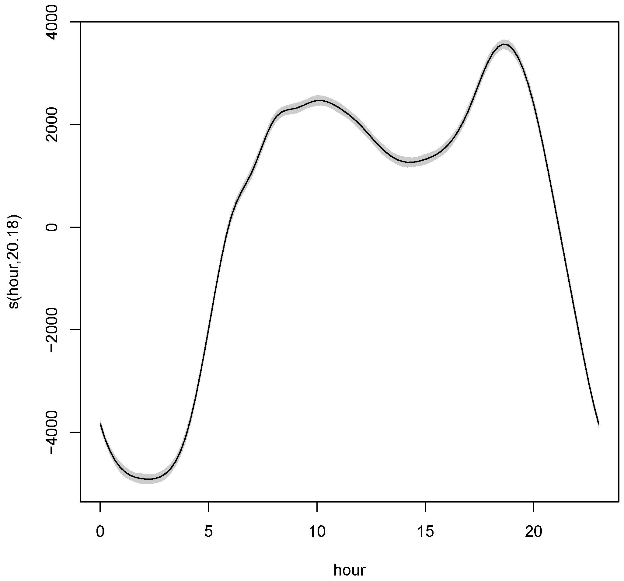
2.2. Generalised Additive Models

Generalised additive models (GAMs) which were developed by Hastie and Tibshirani [27,28] are used in modelling predictors in regression-based models as a sum of smooth functions. The generalised additive model (GAM) is then written as [28,29,30]:

$$g\left(E\left(y_t\right)\right)={\beta }_{0t}+\sum _{i=1}^p{s}_i\left(x_{ti}\right)+{\epsilon }_t.$$

(3)

$y_t$ follows some exponential family distribution, where g denotes a link function and usually the Gaussian link function is used, $s_i$ are smooth functions and ${\epsilon }_t$ is the error term. The smooth function, s is written as

$$s\left(x\right)=\sum _{j=1}^k{\beta }_j{b}_j\left(x\right),$$

(4)

where ${\beta }_j$ denotes the $j^{th}$ parameter, and $b_j\left(x\right)$ represents the $j^{th}$ basis function with the dimension of the basis denoted by k. There are several smoothing spline bases ranging from P-splines, thin plate regression splines, B-splines, cubic regression splines to cyclic cubic regression splines. In this study, we use P-splines and adaptive splines. We seek to find an optimal solution to the optimisation problem given in Equation (5):

$$min\sum _{t=1}^n{\left(y_t-\sum _{i=1}^p{s}_i\left(x_{ti}\right)\right)}^2+\sum _{i=1}^p{\lambda }_i\int {\left(f^{″}\left(x\right)\right)}^{2}dx,$$

(5)

where ${\lambda }_i$ is the $i^{th}$ smoothing parameter.

2.3. The Proposed Models

2.3.1. Additive Quantile Regression Model

An additive quantile regression (AQR) model is a hybrid model that is a combination of GAM and QR models. AQR models were first applied to short-term load forecasting by Gaillard et al. [9] and extended by Fasiolo et al. [10]. Let $y_t$ denote hourly electricity demand where $t=1,\dots ,n$, n is the number of observations and let the number of days be denoted by $n_d$. Then, $n=24n_d$, where 24 is the number of hours in a day and the corresponding p covariates, $x_{t1},x_{t2},\dots ,x_{tp}$. The AQR model is given in Equation (6) [9,10]:

$$y_{t,\tau }=\sum _{j=1}^p{s}_{j,\tau }\left(x_{tj}\right)+{\epsilon }_{t,\tau };\tau \in (0,1),$$

(6)

where $s_{j,\tau }$ are smooth functions and ${\epsilon }_{t,\tau }$ is the error term. The smooth function, s, is written as

$$s_j\left(x\right)=\sum _{k=1}^q{\beta }_{kj}{b}_{kj}\left(x_{tj}\right),$$

(7)

where ${\beta }_j$ denotes the $j^{th}$ parameter, and $b_j\left(x\right)$ represents the $j^{th}$ basis function with the dimension of the basis being denoted by q. The parameter estimates of Equation (6) are obtained by minimising the function given in Equation (8):

$$q_{Y|X}\left(\tau \right)=\sum _{t=1}^n{\rho }_{\tau }\left(y_{t,\tau }-\sum _{j=1}^p{s}_{j,\tau }\left(x_{tj}\right)\right),$$

(8)

where ${\rho }_{\tau }$ is the pinball loss function that is defined in Section 2.1. The AQR models are given in Equations (9) and (10):

$$y_{t,\tau }=\sum _{j=1}^p{s}_{j,\tau }\left(x_{tj}\right)+\sum _{k=1}^K\sum _{j=1}^j{\alpha }_{jk}{s}_j\left(x_{tj}\right)s_k\left(x_{tk}\right)+{\epsilon }_{t,\tau },$$

$$\varphi \left(B\right)\mathsf{\Phi }\left(B^s\right){\epsilon }_{t,\tau }=\theta \left(B\right)\mathsf{\Theta }\left(B^s\right)v_{t,\tau },$$

(9)

$$\Rightarrow \varphi \left(B\right)\mathsf{\Phi }\left(B^s\right)\left[y_{t,\tau }-\left\{\sum _{j=1}^p{s}_{j,\tau }\left(x_{tj}\right)+\sum _{k=1}^K\sum _{j=1}^J{\alpha }_{jk}{s}_j\left(x_{tj}\right)s_k\left(x_{tk}\right)\right\}\right]=\theta \left(B\right)\mathsf{\Theta }\left(B^s\right)v_{t,\tau }.$$

(10)

A comparative analysis will be done with the GAM given in Equation (11) and discussed in Sigauke [31]:

$$y_t={\beta }_{0t}+\sum _{i=1}^p{s}_i\left(x_{ti}\right)+\sum _{k=1}^K\sum _{j=1}^J{\alpha }_{jk}{s}_j\left(x_{tj}\right)s_k\left(x_{tk}\right)+{\epsilon }_t,$$

$$\varphi \left(B\right)\mathsf{\Phi }\left(B^s\right){\epsilon }_t=\theta \left(B\right)\mathsf{\Theta }\left(B^s\right)v_t,$$

(11)

$$\Rightarrow \varphi \left(B\right)\mathsf{\Phi }\left(B^s\right)\left[y_t-\left\{B_{0t}+\sum _{i=1}^p{s}_i\left(x_{ti}\right)+\sum _{k=1}^K\sum _{j=1}^J{\alpha }_{jk}{s}_j\left(x_{tj}\right)s_k\left(x_{tk}\right)\right\}\right]=\theta \left(B\right)\mathsf{\Theta }\left(B^s\right)v_t,$$

(12)

where $y_t$ denotes hourly electricity demand, $s_i$ denotes the smoothing function, $x_{ti}$ represents the covariates, and ${\epsilon }_t$ denotes error terms which are assumed to be autocorrelated. Selection of variables is done using the least absolute shrinkage and selection operator (Lasso) for the hierarchical interactions method developed by Bien et al. [24] and implemented in the R package “hierNet” [32]. The objective is to include an interaction where both variables are included in the model. The restriction known as the strong hierarchy constraint is discussed in detail in Ben and Tibshirani [24] and Lim and Hastie [33].

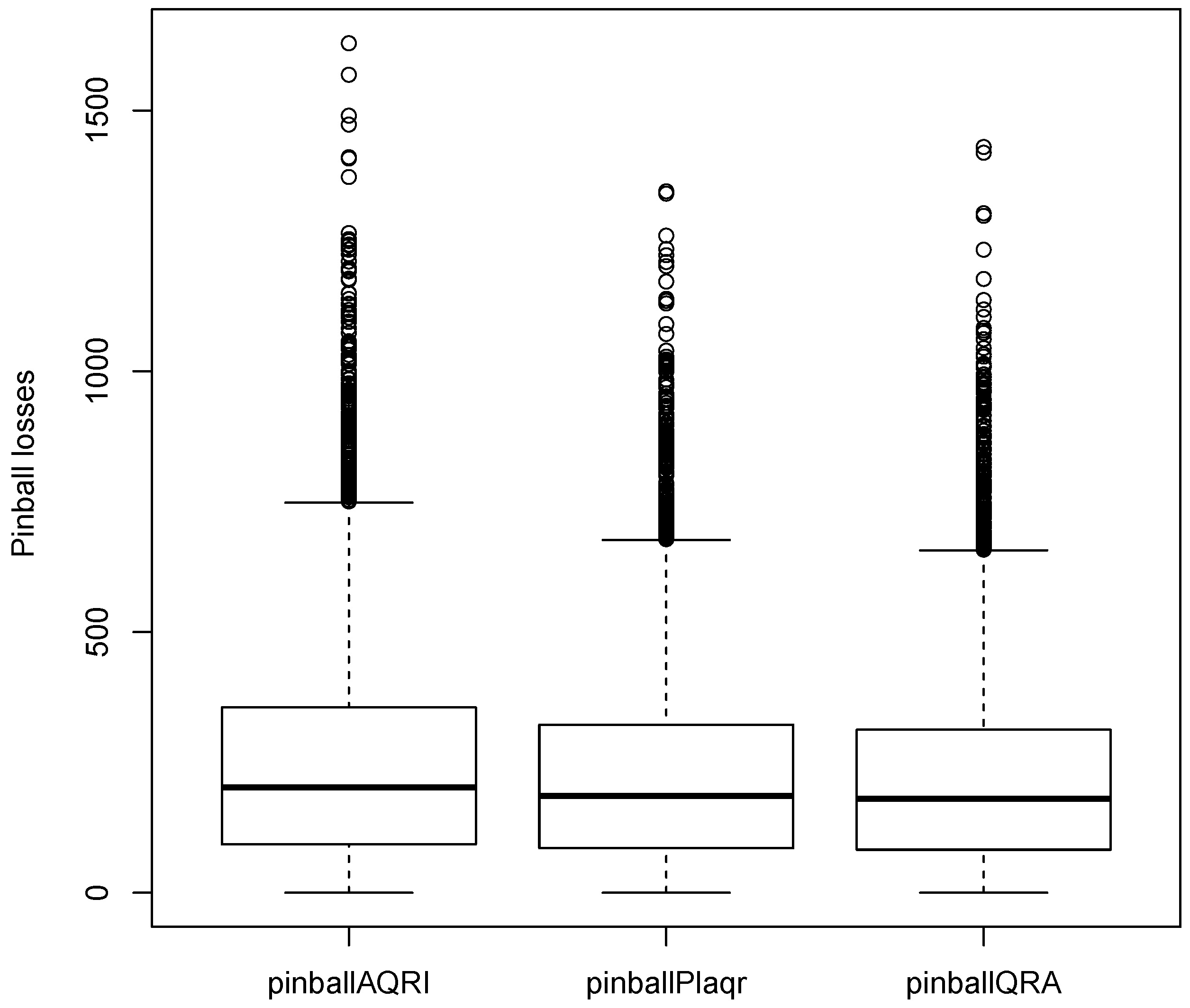
2.3.2. Forecast Error Measures

There are several error measures for probabilistic forecasting which include among others the continuous rank probability score, the logarithmic score and the quantile loss that is also known as the pinball loss. In this paper, we use the pinball loss function which is relatively easy to compute and interpret [34]. The pinball loss function is given as

$$L(q_{\tau },y_t)=\left\{\begin{array}{cc}\tau (y_t-q_t),\hfill & \mathrm{if}{y}_t>q_{\tau },\hfill \\ (1-\tau )(q_{\tau }-y_t),\hfill & \mathrm{if}{y}_t\le q_{\tau },\hfill \end{array}\right.$$

(13)

where $q_{\tau }$ is the quantile forecast and $y_t$ is the observed value of hourly electricity demand.

2.3.3. Percentage Improvement

The percentage improvement between the best model $M_{j\mathrm{best}},j=1,\dots ,k$ with the other models is computed as follows ([35]):

$$\mathrm{Improvement}(\%)=\left(1-\frac{\mathrm{Pinball}\left(\mathrm{best}\mathrm{model}\right)}{\mathrm{Pinball}\left(\mathrm{other}\mathrm{model}\right)}\right)\times 100.$$

(14)

Equation (14) is used to compute the percentage improvements of the best model developed from the other models.

2.3.4. Prediction Intervals

For each of the models, $M_j,j=1,\dots ,k$, we compute the prediction interval widths (PIWs), which we shall abbreviate as ${\mathrm{PIW}}_{ij},i=1,\dots ,n,j=1,\dots ,k$ as follows:

$${\mathrm{PIW}}_{ij}={\mathrm{UL}}_{ij}-{\mathrm{LL}}_{ij},$$

(15)

where ${\mathrm{UL}}_{ij}$ and ${\mathrm{LL}}_{ij}$ are the upper and lower limits of the prediction interval, respectively. The analysis for determining the model which yields narrower PIW is done in this study using box and whisker plots, together with the probability density plots. A comparative analysis is done using the prediction intervals based on QRA [36].

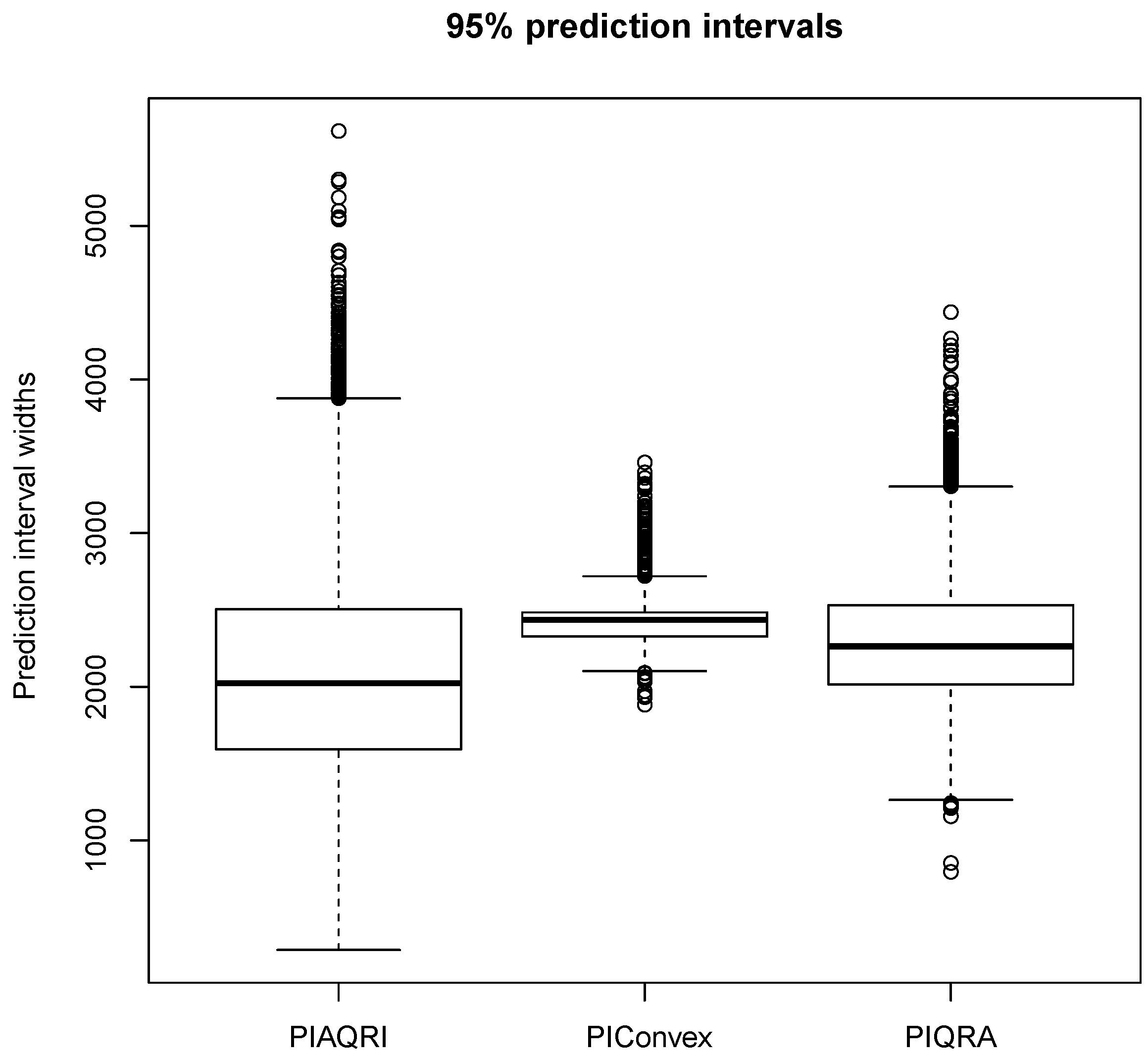
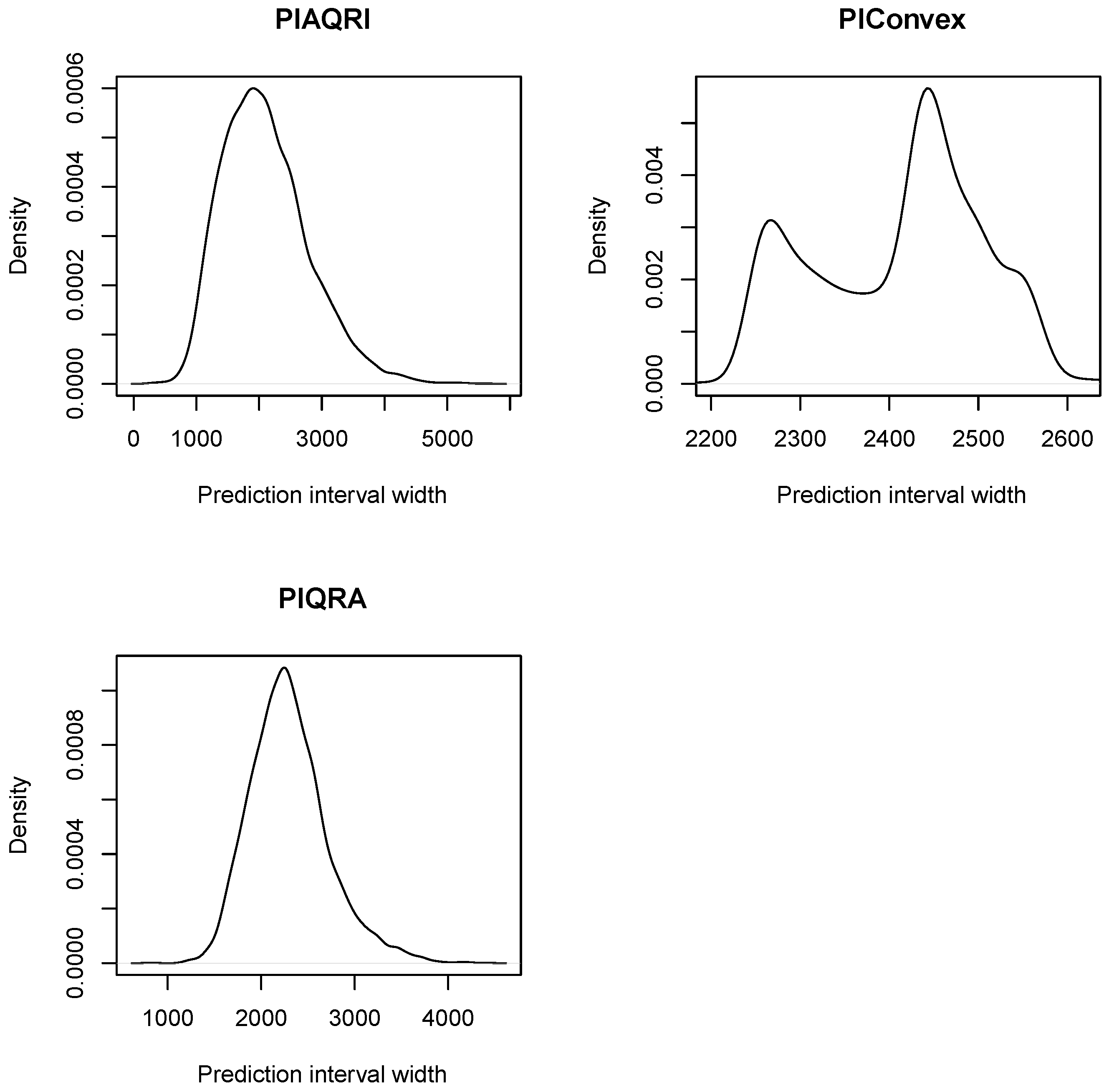
2.3.5. Evaluation of Prediction Intervals

A prediction interval with nominal confidence (PINC) of $100(1-\alpha )\%$ is defined as the probability that the forecast ${\widehat{y}}_{t,\tau }$ lies in the prediction interval $({\mathrm{LL}}_{ij},{\mathrm{UL}}_{ij})$. PINC is given in Equation (16) [37]:

$$\mathrm{PINC}=P\left({\widehat{y}}_{t,\tau }\in ({\mathrm{LL}}_{ij},{\mathrm{UL}}_{ij})\right)=100(1-\alpha )\%.$$

(16)

Various indices are used to evaluate the reliability of prediction intervals (PIs). In this paper, we use the prediction interval coverage probability (PICP), the prediction interval normalised average width (PINAW) and the prediction interval normalised average deviation (PINAD) that are discussed in Sun et al. [37] and Shen et al. [38]. The PICP is given in Equation (17):

$$\mathrm{PICP}=\frac{1}{m}\sum _{i=1}^m{\mathrm{l}}_{ij},$$

(17)

where m is the number of forecasts and I is a binary variable that is defined as

$$I_{ij}=\left\{\begin{array}{cc}1,\hfill & \mathrm{if}{y}_i\in \left({\mathrm{LL}}_{ij},{\mathrm{UL}}_{ij}\right),\hfill \\ 0,\hfill & \mathrm{if}\mathrm{otherwise}.\hfill \end{array}\right.$$

(18)

The PICP is valid if it is greater than or equal to the predetermined level of confidence [37,38]. The PINAW is an index that is used to check if the required value is covered by the prediction interval and is given as follows [37,38]:

$$\mathrm{PINAW}=\frac{1}{m(max\left(y_{ij}\right)-min\left(y_{ij}\right))}\sum _{i=1}^m\left({\mathrm{UL}}_{ij}-{\mathrm{LL}}_{ij}\right),j=1,\dots ,k.$$

(19)

If the PICP is valid and accurate, then the PINAW is usually small [37,38]. However, PINAW can be used to compare different models and then determine the one that possesses the smallest percentage value. Another index which is used to assess the deviation of the target value from the prediction interval is the PINAD, which is given in Equation (20) [37,38]:

$$\mathrm{PINAD}=\frac{1}{m}\sum _{i=1}^m\frac{D_{ij}}{max\left(y_{ij}\right)-min\left(y_{ij}\right)},$$

(20)

where

$$D_{ij}=\left\{\begin{array}{cc}{\mathrm{LL}}_{ij}-y_{ji},\hfill & \mathrm{if}{y}_{ji}<{\mathrm{LL}}_{ij},\hfill \\ 0,\hfill & \mathrm{if}{\mathrm{LL}}_{ij}\le y_{ji}\le {\mathrm{UL}}_{ij},\hfill \\ y_{ji}-U{L}_{ij},\hfill & \mathrm{if}{y}_{ji}>{\mathrm{UL}}_{ij}.\hfill \end{array}\right.$$

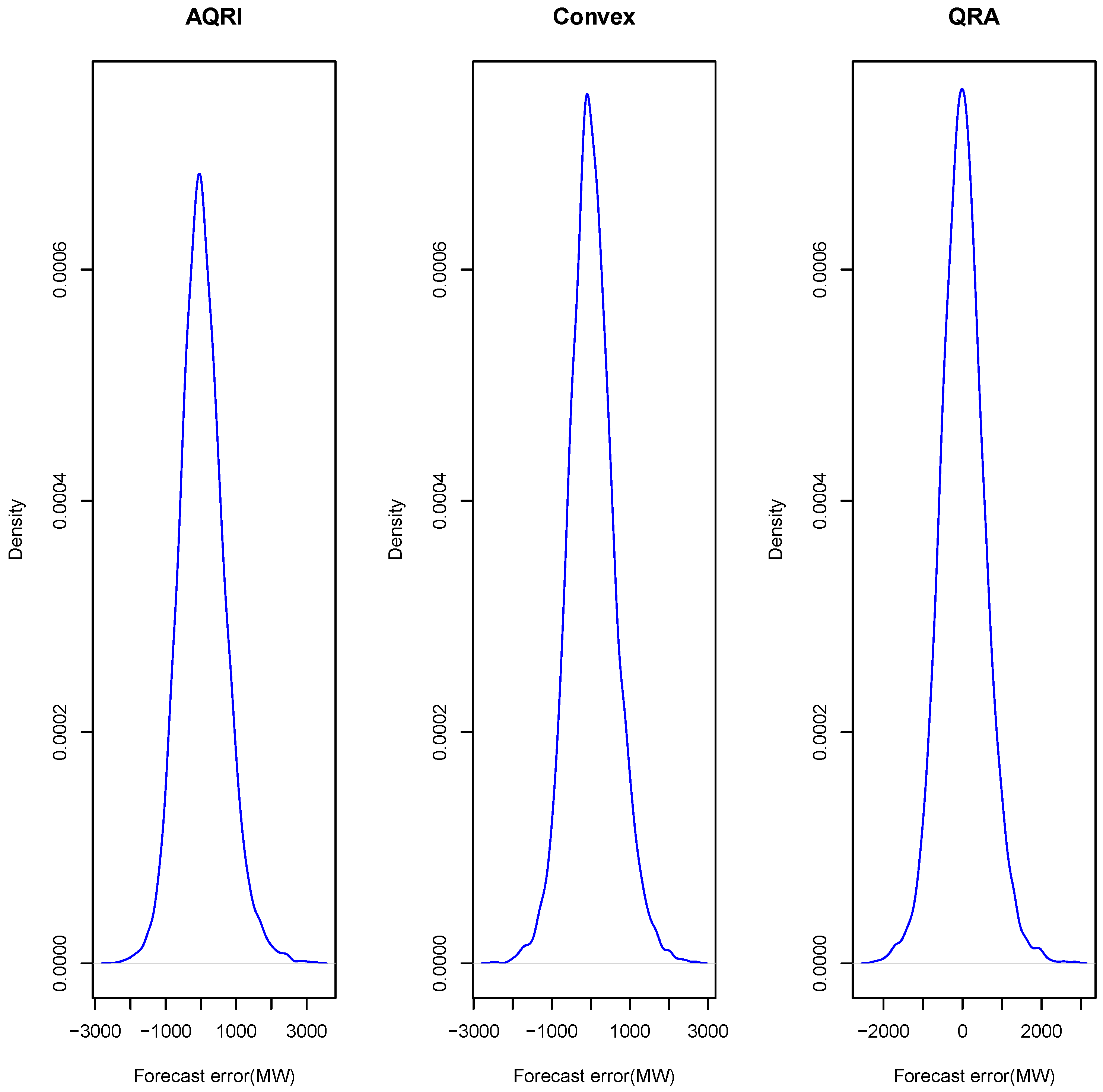
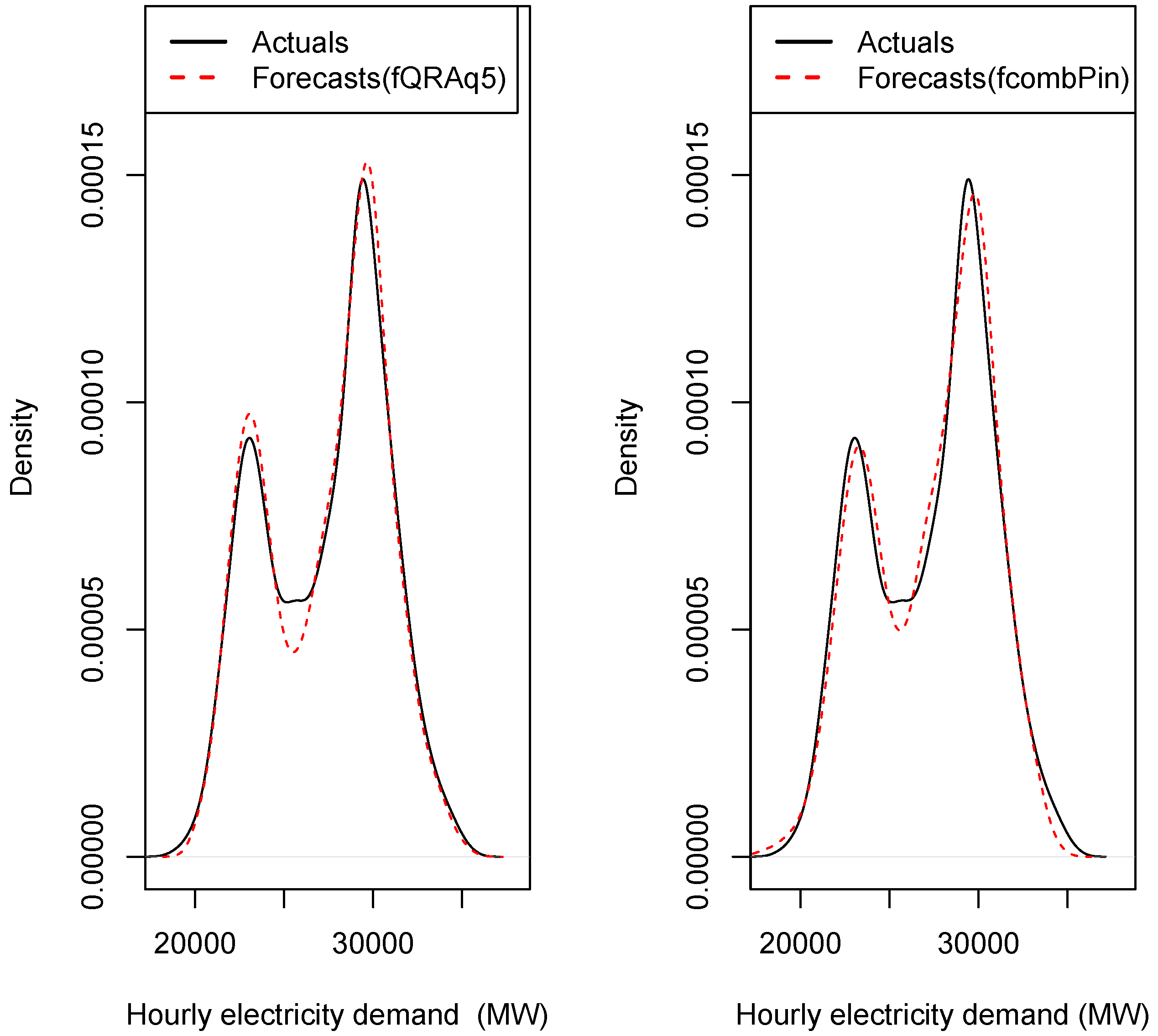
2.3.6. Forecast Error Distribution

For each of the models, $M_j,j=1,\dots ,k$, we extract the residuals ${\epsilon }_{tj}=y_{tj}-{\widehat{y}}_{tj}$ and then compute the under and over predictions. Probability density and box plots of forecast errors including summary statistics are used in the analysis of over and under predictions.

2.3.7. Forecast Combination

QRA is based on forecasting the response variable against the combined forecasts which are treated as independent variables. Let $y_{t,\tau }$ be hourly electricity demand as discussed in Section 2.3.1 and let there be M methods used to predict the next observations of $y_{t,\tau }$, which shall be denoted by $y_{t+1},y_{t+2},\dots ,y_{t+M}$. Using $m=1,\dots ,M$ methods, the combined forecasts will be given by

$${\widehat{y}}_{t,\tau }^{\mathrm{QRA}}={\beta }_0+\sum _{j=1}^k{\beta }_j{\widehat{y}}_{tj}+{\epsilon }_{t,\tau },$$

(21)

where ${\widehat{y}}_{tj}$ represents forecasts from method j, ${\widehat{y}}_{t,\tau }^{\mathrm{QRA}}$ is the combined forecasts and ${\epsilon }_{t,\tau }$ is the error term. We seek to minimise

$$\arg \underset{\beta }{min}\sum _{t=1}^n{\rho }_{\tau }\left({\widehat{y}}_t^{\mathrm{QRA}}-{\beta }_0-\sum _{j=1}^k{\beta }_j{\widehat{y}}_{tj}\right).$$

(22)

In matrix form, we have

$$\arg \underset{\beta \in \mathrm{I}\mathrm{R}}{min}\sum _{t=1}^n{\rho }_{\tau }\left({\widehat{y}}_t^{\mathrm{QRA}}-x_t^T\beta \right),$$

which reduces to

$$\arg \underset{\beta \in {\mathrm{I}\mathrm{R}}^{\rho }}{min}\sum _{t:{\widehat{y}}_t^{\mathrm{QRA}}>x_t^T\beta }\tau \left({\widehat{y}}_t^{QRA}-x_t^T\beta \right)+\sum _{t:{\widehat{y}}_t^{\mathrm{QRA}}<x_t^T\beta }(1-\tau )({\widehat{y}}_t^{\mathrm{QRA}}-x_t^T\beta ).$$

The QRA forecasts will be compared with forecasts based on weighted average of the forecasts given in Equation (23)

$${\widehat{y}}_{t,\tau }^c=\sum _{m=1}^M{\omega }_{mt}{\widehat{y}}_{mt,\tau },$$

(23)

where ${\omega }_{mt}$ is weight assigned to the forecast m.

3. Description of the Case Study

The modelling framework discussed in Section 2 is then applied to a real-life data set. Hourly load data from Eskom, South Africa’s power utility company is used. The data is from all the sectors of the South African economy, i.e., industrial, commercial, agricultural including the residential sectors. In this study, hourly temperature data from the South African Weather Services is used. The temperature data is from 28 meteorological stations. Other variables (predictors) used are lagged demand at lags 1, 12 and 24; including factor variables, hour = 1, hour = 2, ..., hour = 24; month which takes values, month = 1 for January, month = 2 for February, ..., month = 12 for December; daytype taking values daytype = 1 for Monday, daytype = 2 for Tuesday, ..., daytype = 7 for Sunday, variable holiday which takes value 1 if a day is a holiday and also value 1 for a day before and after a holiday. In addition, a nonlinear trend variable is also used.

4. Empirical Results

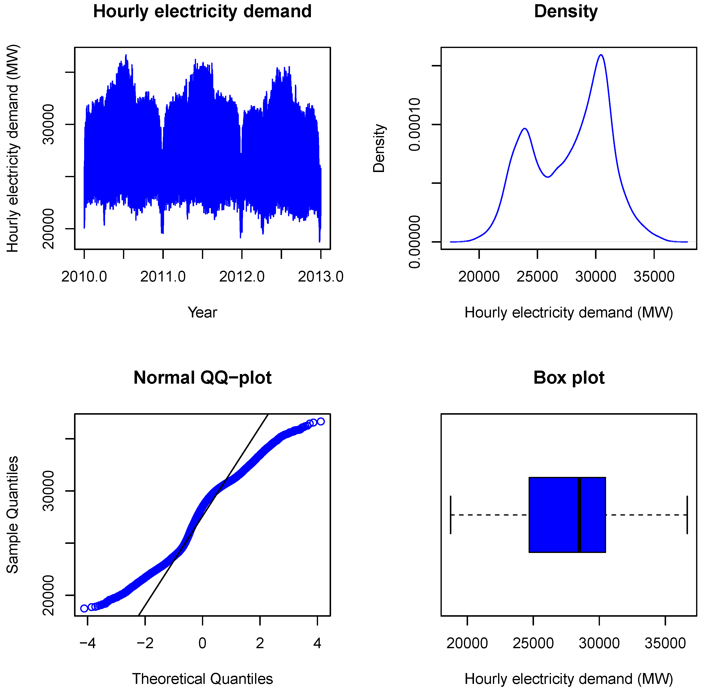
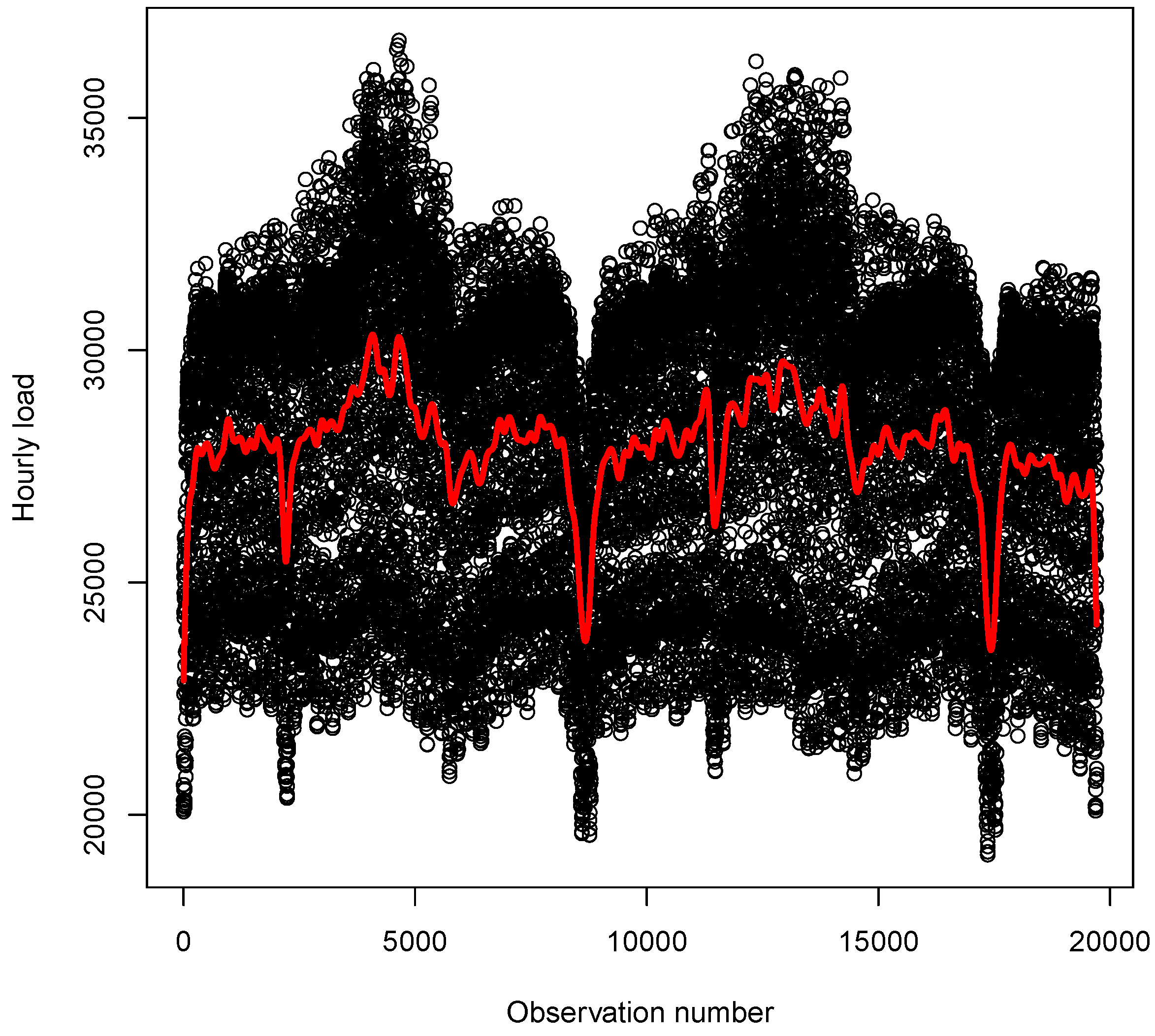
4.1. Exploratory Data Analysis

The summary statistics of hourly electricity demand for the sampling period January 2010 to December 2012 is given in

Table 1. Summary statistics for hourly electricity demand (MW).

Descriptive Statistics	Mean	Median	Max	Min	St. Dev.	Skewness	Kurtosis
Load	27,798	28,496	36,664	18,739	3337	−0.2433	2.050

. The distribution of hourly load is non-normal since it is skewed to the left and platykurtic as shown by the skewness value of −0.243 and a kurtosis value of 2.05 given in Table 1.

Figure 1 shows the time series plot of hourly electricity demand together with density, normal quantile to quantile (Q–Q) and box plots that all show departure from normality of the data. The distribution of the sampling data is bimodal.

A plot of hourly electricity demand with a superimposed nonlinear trend is shown in Figure 2. A penalised cubic regression spline $\pi \left(t\right)={\sum }_{t=1}^n{\left(y_t-f\left(x_t\right)\right)}^2+\lambda \int {\left(f^{″}\left(x\right)\right)}^{2}dx$ is used as the nonlinear trend function, with $\lambda$ as the smoothing parameter and is estimated by generalised cross-validation (GCV) approach. The fitted values are extracted and used as input values for the nonlinear trend variable in the GAM and AQR models.

4.2. Forecasting Electricity Demand When Covariates Are Known in Advance

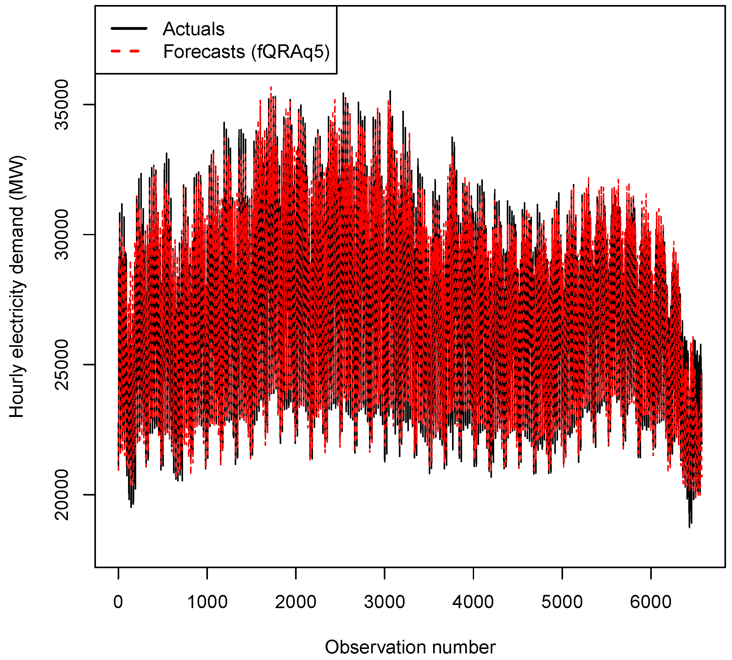
4.2.1. Forecasting Results

The data used is hourly electricity demand from 1 January 2010 to 31 December 2012 giving us $n=$ 26,281 observations. The data is split into training data, 1 January 2010 to 2 April 2012, i.e., $n_1=$ 19,708 and testing data, from 2 April 2012 to 31 December 2012, i.e., $n_2=6573$, which is $25\%$ of the total number of observations. The smoothed effect of the variable “hour” which is given in Figure 3 shows that daily peak electricity demand occurs around 7:00 p.m. The period 5:00 p.m. to 9:00 p.m. is then considered as the peak period in which electricity demand is expected to exceed a certain high threshold, which is likely to cause problems for the system operators due to grid instability and severe stress on the system.

The models considered are $M_1$ (GAM), $M_2$ (GAMI), which are GAM models without and with interactions, respectively, and $M_3$ (AQR), $M_4$ (AQRI) which are additive quantile regression models without and with interactions, respectively. The four models $M_1$ to $M_4$ are then combined based on the pinball losses, resulting in $M_5$ and also combined using QRA, resulting in $M_6$.

4.2.2. Out of Sample Forecasts

After correcting for residual autocorrelation, we then use the model for out of sample forecasting (testing). A comparative analysis of the models given in

Table 2. Model comparisons.

	${\mathit{M}}_1$	${\mathit{M}}_2$	${\mathit{M}}_3$	${\mathit{M}}_4$	${\mathit{M}}_5$	${\mathit{M}}_6$
RMSE	736.2	662.4	731.5	648.8	596.1	577.7
MAE (NW)	568.7	516.2	549.5	499.7	459.4	445.2
MAPE (%)	2.15	1.93	2.04	1.86	1.70	1.65
Under predictions				3319	3279	3280
Over predictions				3251	3291	3286

shows that $M_4$ is the best model out of the four models, $M_1$ to $M_4$, based on the root mean square error (RMSE), mean absolute error (MAE) and mean absolute percentage error (MAPE). The forecasts from the four models are then combined based on the pinball losses. The weights assigned to the forecasts from the models $M_1$ to $M_4$ are 0.0174, 0.0946, 0.326 and 0.562, respectively. The model for combining the forecasts based on the pinball losses is $M_5$. Model $M_6$, i.e., the model based on QRA has the lowest MAE and MAPE values as shown in Table 2. Model 4 has more under predictions compared to over predictions, and $M_5$ has more over predictions compared to under predictions, while, for model 6, the under and over-predictions are almost the same.

Using models $M_4$, $M_5$ and $M_6$, we then compute the average pinball losses. The average losses suffered by the models based on the pinball losses are given in

Table 3. Average pinball losses for $M_1$ to $M_6$ (2 April 2012 to 31 December 2012).

	${\mathit{M}}_1$	${\mathit{M}}_2$	${\mathit{M}}_3$	${\mathit{M}}_4$	${\mathit{M}}_5$	${\mathit{M}}_6$
Average Pinball loss	284.363	258.087	274.768	249.842	229.723	222.584

with model $M_6$ having the smallest average pinball loss.

In order to test the effectiveness of the forecasting models $M_4$ to $M_6$, we present, in Figure 4, box plots of the pinball loses of the models.

4.2.3. Evaluation of Prediction Intervals

Empirical prediction intervals (PIs) are constructed using the forecasts from the models $M_4$ to $M_6$. The constructed PIs are then used to find PIWs, PINAWs, PINADs and calculation of the number of forecasts below and above the PIs from each model. Summary statistics of the PIWs for the models $M_4$ to $M_6$ for PINC value of $95\%$ are given in

Table 4. Model comparisons.

	Mean	Median	Minimum	Maximum	Standard Deviation	Skewness	Kurtosis	Range
$M_4$	2100.9	2023	287	5617	686.98	0.7256	3.7217	5330
$M_5$	2419.1	2435	1883	3560	117.72	1.4898	12.3368	1667
$M_6$	2300.0	2263	795	4438	418.11	0.6776	4.0304	3643

. The distributions of the PIWs for the three models are all leptokurtic since they are greater than 3. They are all skewed to the right since the values of their skewness are all positive. This shows that heavy-tailed distributions would be appropriate to fit the distributions of the PIWs of the three models. Model $M_5$ has the smallest standard deviation, which indicates narrower PIW compared to $M_4$ and $M_6$.

Boxplots of widths of the PIs for the forecasting models $M_4$, $M_5$ and $M_6$ are given in Figure 5. The figure shows that the PI from model M5 are narrower compared to those from M4 and M6.

Figure 6 shows the density plots of the PIWs of $M_4$, $M_5$ and $M_6$. The distribution of the PIWs of $M_5$ is bimodal and all the densities show that the distributions are skewed to the right.

In order to choose the best model based on the analysis of the PIWs, we need to calculate the PICPs, PINAWs and PINADs including a count of the number of forecasts below and above the PIs. This is done for various PINC values, which are $90\%$, $95\%$ and $99\%$, respectively. A comparative evaluation of the models using PI indices for PINC values of $90\%$, $95\%$ and $99\%$ are given in

Table 5. Comparative evaluation of models using prediction interval (PI) indices. Below LL = number of forecasts below the lower prediction limit, Above UL = number of forecasts above the upper prediction limit.

PINC	Model	PICP (%)	PINAW (%)	PINAD (%)	Below LL	Above UL
$90\%$	$M_4$	84.41	10.63	0.2353	462	563
	$M_5$	90.46	11.73	0.1671	310	317
	$M_6$	90.80	11.07	0.1347	301	304
$95\%$	$M_4$	91.19	12.52	0.1186	236	343
	$M_5$	95.16	14.41	0.0756	156	162
	$M_6$	95.31	13.70	0.0573	151	157
$99\%$	$M_4$	97.35	16.43	0.03127	36	138
	$M_5$	99.1	19.87	0.0110	30	31
	$M_6$	99.22	17.75	0.005986	31	20

. Models $M_5$ and $M_6$ have valid PICPs for the three PINC values, with $M_6$ having the highest PICP. Model $M_6$ has the smallest PINAD values and fewer number of forecasts falling below and above the PIs. Model $M_4$ has the smallest PINAW value for all three of the PINC values. All three of the models could be used in the construction of PIs. Although $M_4$ does not give a valid PICP, the PINAW and PINAD are reasonably small. The performance of model $M_6$ seems to be the best amongst these three models. However, this analysis is not enough and, as a result, we need further analysis using residuals of the three models.

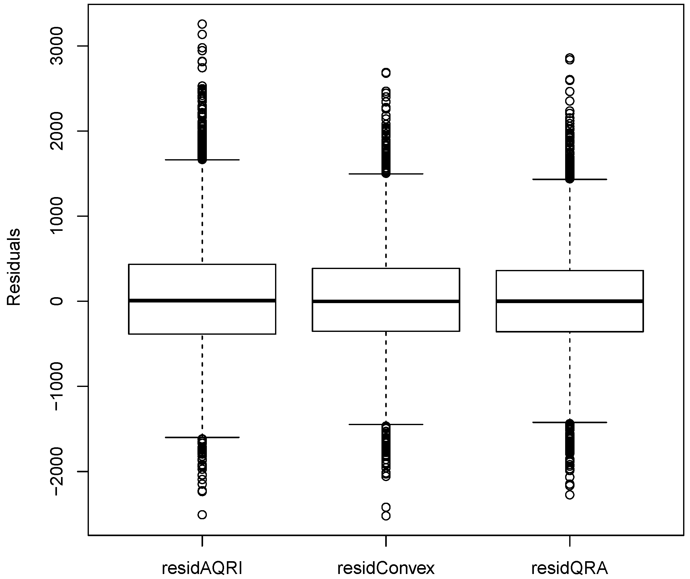
4.2.4. Residual Analysis

Table 6. Model comparisons.

	Mean	Median	Minimum	Maximum	Standard Deviation	Skewness	Kurtosis
$M_4$	44.16	7	−2507	3258	647.36	0.3761	3.9266
$M_5$	28.55	−1	−2520	2690	595.49	0.2442	3.7702
$M_6$	14.98	0	−2273	2860	577.56	0.1997	3.9223

gives summary statistics of the residuals from the models $M_4$, $M_5$ and $M_6$. Model $M_6$ has the smallest standard deviation with a median of zero, showing that it is the best model for predicting hourly electricity demand. All three of the models have positive skewness, an indication of a large number of positive errors, which is a reflection of underestimation of predicted hourly electricity demand. Model 6 has the smallest skewness value. A failure to predict high electricity demand is shown by high values of kurtosis [16]. The kurtosis values of all three of the models are greater than 3.

The error distributions of each of the forecasting models $M_4$, $M_5$ and $M_6$ are given in Figure 7, which shows that the number of positive errors dominates negative errors, an indication that the distribution of errors for each of the three models is positively skewed. Model $M_6$ is the best fitting model since it has the smallest distribution of errors.

Figure 8 shows the boxplots of the hourly errors from the three models. The range of the errors from M6 is narrower compared to the ones from M4 and M5.

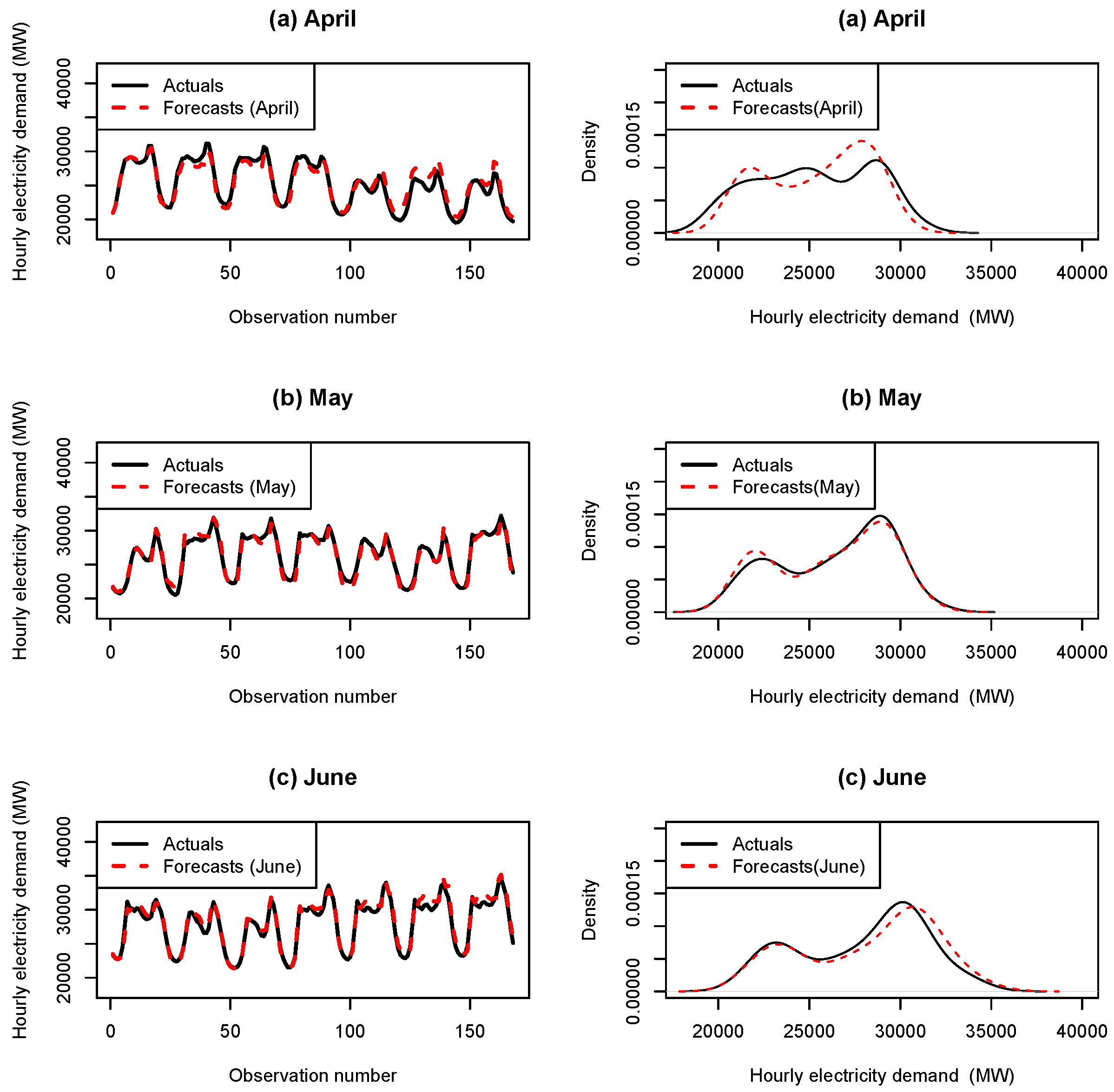
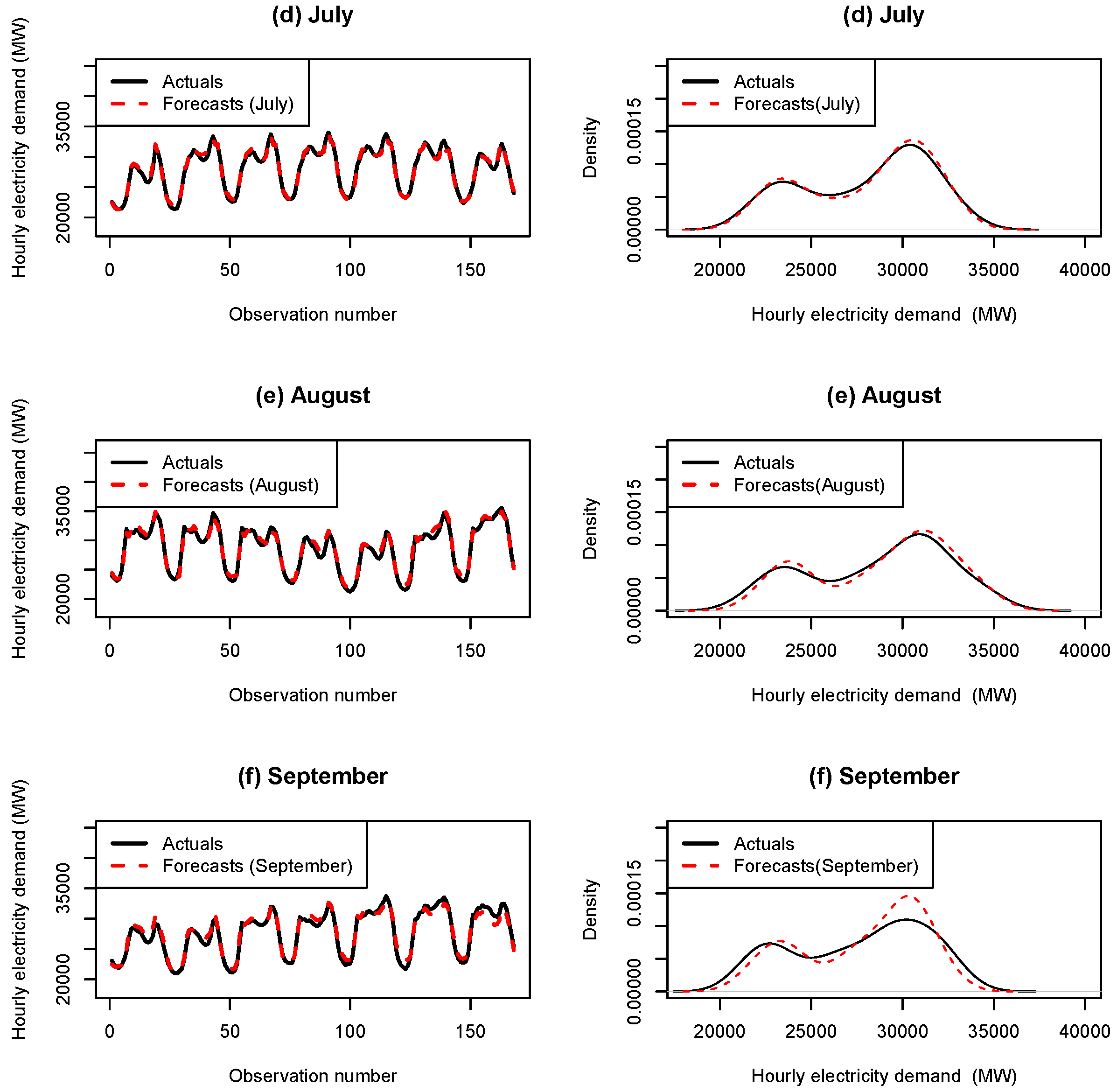
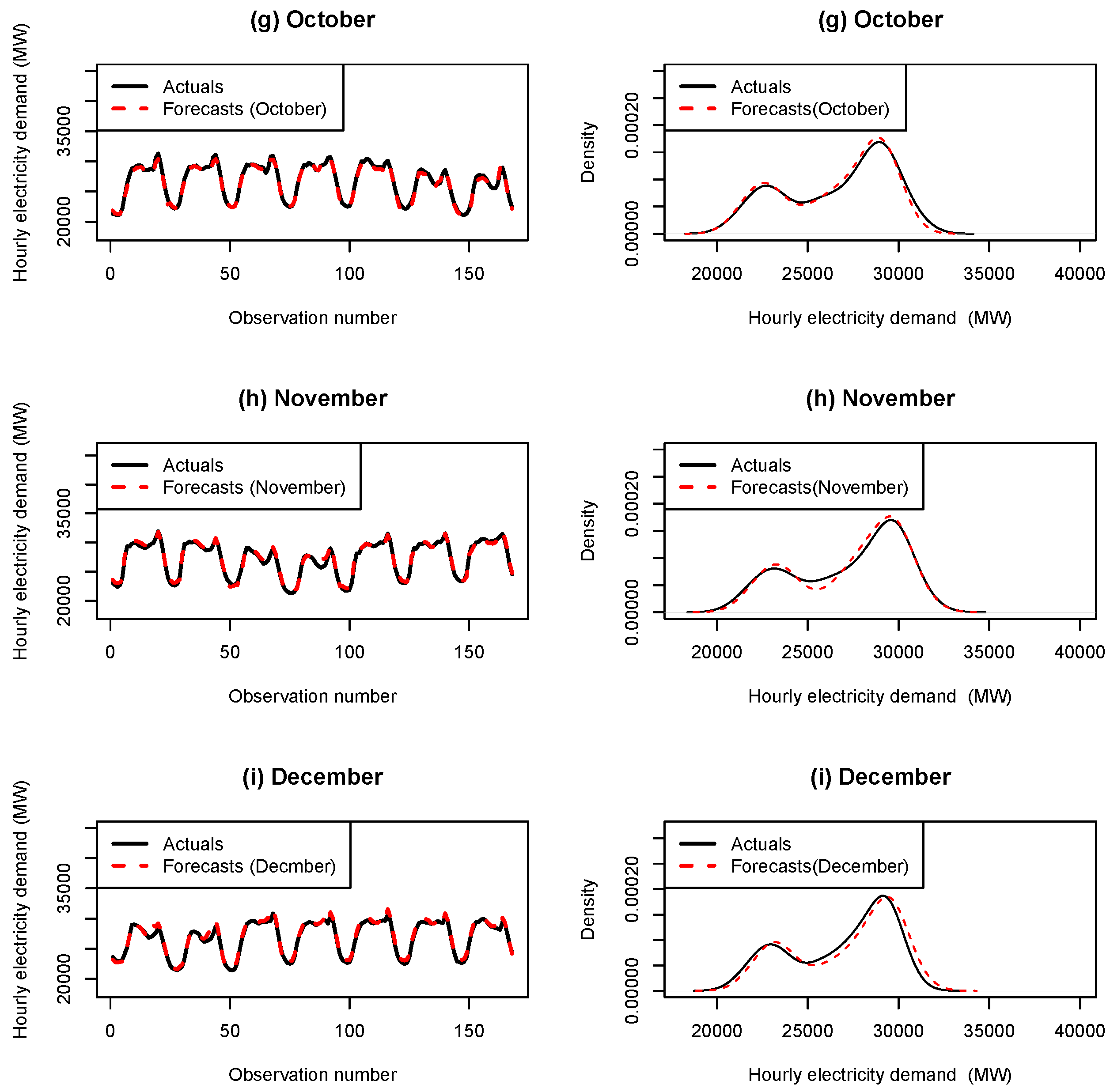
4.2.5. Plots of out of Sample Forecasts

From the analysis of the PIWs and residual analysis, $M_6$ is the best fitting model and can be used for predicting hourly electricity demand. The plot of actual demand superimposed with forecasted demand from model $M_6$ (2 April to 31 December 2012) given in Figure 9 shows that the forecasts follow hourly electricity demand very well.

The density plots from $M_6$ (QRA forecasts) and $M_5$ (convex combination forecasts) models superimposed with actual hourly electricity demand are given in Figure 10. In both plots, the fit of the densities is fairly good.

A summary of the accuracy measures for the months April to December 2012 for each of the first 168 forecasts of each month is given in

Table A1. Forecast accuracy measures root mean square error (RMSE), mean absolute error (MAE) and mean absolute percentage error (MAPE) for the forecasts of April to December 2012.

	RMSE	MAE (MW)	MAPE (%)
April	945.5214	781.6429	3.151406
May	620.7605	488.6548	1.891559
June	665.0797	537.5238	1.898156
July	392.0611	329.3393	1.181808
August	642.6158	538.2321	1.903814
September	750.3948	618.5476	2.264714
October	345.0181	271.0595	1.010533
November	394.3301	302.9048	1.146244
December	468.6219	369.5595	1.395704

in Appendix A while Appendix B shows in Figure A1, Figure A2 and Figure A3 hourly load superimposed with forecasts together with their respective densities.

5. Discussion

The modelling approach discussed in this study allows for easy interpretability and accounting for residual autocorrelation in the joint modelling of hourly electricity data. A comparative analysis was then done with the generalised additive models (GAMs). In both modelling frameworks, variable selection was done using Lasso via hierarchical interactions. Four models considered were GAMs and AQR models with and without interactions. The AQR model with pairwise interactions was found to be the best fitting model. The forecasts from the four models were then combined using an algorithm based on the pinball loss (convex combination model) and also using quantile regression averaging (QRA). The AQR model with interactions was then compared with the convex combination and QRA models and the QRA model gave the most accurate forecasts. Except for the AQR model with interactions, the other two models’ convex combination model and the QRA model gave prediction interval coverage probabilities which were valid for the $90\%$, $95\%$ and the $99\%$ prediction intervals. The QRA model had the smallest prediction interval normalised average width and prediction interval normalised average deviation.

6. Conclusions

This study discussed an application of short-term hourly electricity demand forecasting in South Africa using additive quantile regression (AQR) models without and with pairwise interactions which satisfy the strong hierarchy in Lasso via hierarchical interactions. This modelling approach allows for a detailed analysis which goes beyond the performance statistics in forecasting. This approach has merit in that it gives more insight in the developed models.

References

1. Maciejowska, K.; Weron, R. Forecasting of daily electricity prices with factor models: Utilizing intra-day and inter-zone relationships. Comput. Stat. 2017, 30, 805–819. [Google Scholar] [CrossRef]
2. Wood, S.N.; Goude, Y.; Shaw, S. Generalized additive models for large datasets. J. R. Stat. Soc. 2015, 64, 139–155. [Google Scholar] [CrossRef] [Green Version]
3. Tsay, R.S. Analysis of Financial Time Series, 2nd ed.; Wiley Series in Probability and Statistics; Wiley Online Library: Hoboken, NJ, USA, 2005. [Google Scholar]
4. Dordonnat, V.; Koopman, S.J.; Ooms, M. Dynamic factors in periodic time-varying regressions with an application to hourly electricity load modelling. Comput. Stat. Data Anal. 2012, 56, 3134–3152. [Google Scholar] [CrossRef]
5. Soares, L.J.; Medeiros, M.C. Modeling and Forecasting Short-term Electric Load Demand: A Two-Step Methodology. 2016. Available online: https://pdfs.semanticscholar.org/734b/3f6565243912784ad7b1a7421acb7188c9ca.pdf (accessed on 28 December 2016).
6. Ramanathan, R.; Engle, R.; Granger, C.W.J.; Vahid-Araghi, F.; Brace, C. Short-run forecasts of electricity loads and peaks. Int. J. Forecast. 1997, 13, 161–174. [Google Scholar] [CrossRef]
7. Fan, S.; Hyndman, R.J. Short-term load forecasting based on a semi-parametric additive model. IEEE Trans. Power Syst. 2012, 27, 134–141. [Google Scholar] [CrossRef]
8. Goude, Y.; Nedellec, R.; Kong, N. Local short and middle term electricity load forecasting with semi-parametric additive models. IEEE Trans. Smart Grid 2014, 5, 440–446. [Google Scholar] [CrossRef]
9. Gaillard, P.; Goude, Y.; Nedellec, R. Additive models and robust aggregation for GEFcom2014 probabilistic electric load and electricity price forecasting. Int. J. Forecast. 2016, 32, 1038–1050. [Google Scholar] [CrossRef]
10. Fasiolo, M.; Goude, Y.; Nedellec, R.; Wood, S.N. Fast Calibrated Additive Quantile Regression. 2017. Available online: https://github.com/mfasiolo/qgam/blob/master/draftqgam.pdf (accessed on 13 March 2017).
11. Laouafi, A.; Mordjaoui, M.; Haddad, S.; Boukelia, T.E.; Ganouche, A. Online electricity demand forecasting based on effective forecast combination methodology. Electr. Power Syst. Res. 2017, 148, 35–47. [Google Scholar] [CrossRef]
12. Zhang, X.; Wang, J.; Zhang, K. Short-term electric load forecasting based on singular spectrum analysis and support vector machine optimized by Cuckoo search algorithm. Electr. Power Syst. Res. 2017, 146, 270–285. [Google Scholar] [CrossRef]
13. Boroojeni, K.G.; Amini, M.H.; Bahrami, S.; Iyengar, S.S.; Sarwat, A.I.; Karabasoglu, O. A novel multi-time-scale modelling for electric power demand forecasting: From short-term to medium-term horizon. Electr. Power Syst. Res. 2017, 142, 58–73. [Google Scholar] [CrossRef]
14. Khwaja, A.S.; Zhang, X.; Anpalagan, A.; Venkatesh, B. Boosted neural networks for improved short-term electric load forecasting. Electr. Power Syst. Res. 2017, 143, 431–437. [Google Scholar] [CrossRef]
15. Ekonomou, L.; Christodoulou, C.A.; Mladenov, V. A short-term load forecasting method using artificial neural networks and wavelet analysis. Int. J. Power Syst. 2016, 1, 64–68. [Google Scholar]
16. Pappas, S.S.; Ekonomou, L.; Moussas, V.C.; Karampelas, P.; Katsikas, S.K. Adaptive load forecasting of the Hellenic electric grid. J. Zhejiang Univ. Sci. A 2008, 9, 1724–1730. [Google Scholar] [CrossRef]
17. Gajowwniczek, K.; Zabkowski, T. Two-stage electricity demand modeling using machine learning algorithms. Energies 2017, 10, 1547. [Google Scholar] [CrossRef]
18. Chapgain, K.; Kittipiyakul, S. Performance analysis of short-term electricity demand with atmospheric variables. Energies 2018, 11, 818. [Google Scholar] [CrossRef]
19. Divina, F.; Gilson, A.; Goméz-Vela, F.; Torres, M.G.; Torres, J.F. Stacking ensemble learning for short-term electricity consumption forecasting. Energies 2018, 11, 949. [Google Scholar] [CrossRef]
20. Nagbe, K.; Cugliari, J.; Jacques, J. Short-term electricity demand forecasting using a functional state space model. Energies 2018, 11, 1120. [Google Scholar] [CrossRef]
21. Chikobvu, D.; Sigauke, C. Regression-SARIMA modelling of daily peak electricity demand in South Africa. J. Energy S. Afr. 2012, 23, 23–30. [Google Scholar]
22. Sigauke, C.; Chikobvu, D. Short-term peak electricity demand in South Africa. Afr. J. Bus. Manag. 2012, 6, 9243–9249. [Google Scholar] [CrossRef]
23. Sigauke, C.; Chikobvu, D. Peak electricity demand forecasting using time series regression models: An application to South African data. J. Stat. Manag. Syst. 2016, 19, 567–586. [Google Scholar] [CrossRef]
24. Bien, J.; Taylor, J.; Tibshirani, R. A lasso for hierarchical interactions. Ann. Stat. 2013, 41, 1111–1141. [Google Scholar] [CrossRef] [PubMed]
25. Laurinec, P. Doing Magic and Analyzing Seasonal Time Series with GAM, (Generalized Additive Model) in R. 2017. Available online: https://petolau.github.io/Analyzing-double-seasonal-time-series-with-GAM-in-R/ (accessed on 23 February 2017).
26. Koenker, R.; Bassett, G. Regression quantiles. Econ. J. Econ. Soc. 1978, 46, 33–50. [Google Scholar] [CrossRef]
27. Hastie, T.; Tibshirani, R. Generalized additive models (with discussion). Stat. Sci. 1986, 1, 297–318. [Google Scholar] [CrossRef]
28. Hastie, T.; Tibshirani, R. Generalized Additive Models; Chapman & Hall: London, UK, 1990. [Google Scholar]
29. Wood, S.N. Generalized Additive Models: An Introduction with R; Chapman & Hall: London, UK, 2006. [Google Scholar]
30. Wood, S.N. Generalized Additive Models: An Introduction with R; Chapman & Hall: London, UK, 2017. [Google Scholar]
31. Sigauke, C. Forecasting medium-term electricity demand in a South African electric power supply system. J. Energy S. Afr. 2017, 28, 54–67. [Google Scholar] [CrossRef]
32. Bien, J.; Tibshirani, R. R Package “HierNet”, Version 1.6. 2015. Available online: https://cran.r-project.org/web/packages/hierNet/hierNet.pdf (accessed on 22 May 2017).
33. Lim, M.; Hastie, T. Learning interactions via hierarchical group-lasso regularization. J. Comput. Graph. Stat. 2015, 24, 627–654. [Google Scholar] [CrossRef] [PubMed] [Green Version]
34. Hong, T.; Pinson, P.; Fan, S.; Zareipour, H.; Troccoli, A.; Hyndman, R.J. Probabilistic energy forecasting: Global Energy Forecasting Competition 2014 and beyond. Int. J. Forecast. 2016, 32, 896–913. [Google Scholar] [CrossRef] [Green Version]
35. Abuella, M.; Chowdhury, B. Hourly probabilistic forecasting of solar power. In Proceedings of the 49th North American Power Symposium, Morgantown, WV, USA, 17–19 September 2017. [Google Scholar]
36. Liu, B.; Nowotarski, J.; Hong, T.; Weron, R. Probabilistic load forecasting via quantile regression averaging of sister forecasts. IEEE Trans. Smart Grid 2017, 8, 730–737. [Google Scholar] [CrossRef]
37. Sun, X.; Wang, Z.; Hu, J. Prediction interval construction for byproduct gas flow forecasting using optimized twin extreme learning machine. Math. Probl. Eng. 2017. [Google Scholar] [CrossRef]
38. Shen, Y.; Wang, X.; Chen, J. Wind power forecasting using multi-objective evolutionary algorithms for wavelet neural network-optimized prediction intervals. Appl. Sci. 2018, 8, 185. [Google Scholar] [CrossRef]
Figure 1. Hourly electricity demand from January 2010 to 31 December 2012.
Energies 11 02208 g001
Figure 2. Plot of hourly electricity demand from 1 January 2010 to 31 December 2012 superimposed with a nonlinear trend.
Energies 11 02208 g002
Figure 3. Smoothed effects of variable “hour”.
Energies 11 02208 g003
Figure 4. Plot of pinball losses for models M 4 (pinballAQRI), M 5 (pinballPlaqr) and M 6 (pinballQRA) (2 April 2012 to 31 December 2012).
Energies 11 02208 g004
Figure 5. Prediction interval widths for models M 4 (PIAQRI), M 5 (PIConvex) and M 6 (PIQRA).
Energies 11 02208 g005
Figure 6. Density plots of the prediction interval widths for models M 4 (PIAQRI), M 5 (PIConvex) and M 6 (PIQRA).
Energies 11 02208 g006
Figure 7. The error distribution of forecasting techniques for M4(AQRI), M5(convex) and M6(QRA).
Energies 11 02208 g007
Figure 8. Box plots of residuals from models M 4 (residAQRI), M 5 (residConvex) and M 6 (residQRA).
Energies 11 02208 g008
Figure 9. Plot of actual demand superimposed with forecasted demand from M 6 (2 April to 31 December 2012).
Energies 11 02208 g009
Figure 10. Density plots of actual demand superimposed with density plots from M 6 and M 5 models (2 April to 31 December 2012).
Energies 11 02208 g010