Abstract
A city bus with hybrid drive system was studied for its performance. The driveline under consideration consists of two alternative energy sources—an internal combustion engine (ICE) and kinetic energy storage (KES)—a hydrostatic transmission (HST), a drive axle and corresponding gears. A generalized law for HST control is obtained that satisfies kinematic and torque requirements for the alternative energy sources and the different modes of operation of the bus. A test stand was developed for validation of the chosen control strategy and for the energy flow simulations through the HST. The estimated maximum energy recovery potential is around 20–25%.
1. Introduction
Efficient energy use is a problem of current interest. Operation of heavy-duty vehicles in non-steady moving modes, such as a city bus, for example, is connected to proven inefficient energy use. The energy for vehicle acceleration and the kinetic energy of the moving vehicle are lost as heat in the conventional brake system. If a recuperation device is built into the vehicle driveline, it would allow the accumulation of a significant part of the kinetic energy during brake modes.
Different types of recuperation devices are known [1], but the most competitive ones are electro-chemical storage (electric batteries), kinetic energy storage or flywheels (KES), and potential energy storage (hydro-accumulators). All of them have their pros and cons, but because of the necessity of high peaks of power density for heavy-duty applications, the most attractive storage devices are KES. The idea of KES usage as an energy buffer for vehicular application has almost 70 years of history, starting with the Gyrobus manufactured by Oerlikon [2], and the review in [3] gives its evolution over years. KES utilization has gained popularity with the systems in Formula (1) [4] and is evolving from prototypes [5] to mass production [6] in cars. A comparative analysis of several types of energy storage devices, presented in [7], indicates that higher fuel economy can be achieved by KES on heavy duty modes of vehicle operation. According to [8], KES technology has reached its maturity, with 500 flywheel power buffer systems being deployed for London buses. Battery utilization for heavy vehicles has been reported recently by Tesla and Volvo [9,10], which means that the technology already exists, but comes at the expense of higher cost and increased overall mass, because of the battery’s own weight, relative to the necessary energy capacity.
The main challenge of KES usage is the necessity of power transmission across a continuous range of speed ratios [11]. Different types of continuously variable transmissions (CVT) are available, but the choice of energy device type is inevitably coupled with the choice of the transmission type according to the requirements for less or no energy conversion. The most appropriate and simplest CVT types of KES utilization are mechanical ones, such as the V-belt drive [12,13], combined automated manual transmission (AMT) with belt variators as CVT [14], and AMT transmission with toroidal CVT [15], where the latter is the basis of London buses [16]. The weak point of such transmission configurations is the power flow limit through the CVT part, and as a consequence, the inability to use KES in its optimal efficiency range [17]. Based on the achievement of the popular Toyota Prius hybrid drive line [18], power-split continuous variable transmissions (PSCVTs) of various types are considered to be a promising variant in future for KES coupling [19]. Mechanical CVT used in parallel with planetary gear sets and KES was considered for a Zero Inertia powertrain in [20], in which a sophisticated control algorithm was proposed for KES utilization in transient modes. A dual planetary set with appropriate brake and clutch control or with V-belt CVT as a closed loop was proposed in [21], and the authors predicted a 27.5% fuel economy improvement. A two-mode power transmission with hydrostatic and hydromechanical branches and KES has been used in a MAN (Maschinenfabrik Augsburg-Nürnberg) bus prototype [22], but because of the increased complexity such transmissions are abandoned.
The electric drive, consisting of electric machines capable of transferring power in both motor and generator modes, has its place in CVT transmissions with KES [23]. The necessity of double energy conversion from mechanical to electrical and from electrical to mechanical form reduces the overall efficiency when KES is used as an energy storage device, and such electric transmissions take place in hybrid vehicles with battery storage systems, or in hybrid electric drives with KES as an energy buffer [17].
Hydrostatic transmission (HST) with variable displacement pumps and motors is the next candidate for infinite CVT for hybrid vehicles with KES. The similarity with electric transmission is evident with regard to the necessity for double energy conversion, and hydro-accumulators are usually used as storage devices. A big advantage of such transmissions is their mass producibility [24,25]. Hydraulic hybrids incorporating hydro-accumulator have an established position nowadays [26], but the author claims there is still a great need for improved component performance and improvement of the control systems. Moreover, the control of HST is still much more complex than the control of electric hybrids. However, according to [27], HSTs with secondary control systems using a constant pressure system (CPS) combined with KES, secondary control systems using impressed pressure with a hydro-accumulator, and electro-hydraulic actuators have been considered as energy-saving systems. One approach to overriding the low energy density of the hydro-accumulator is to integrate the hydro-accumulator and KES by allowing the hydro-accumulator to rotate, which leads to the so-called “Flywheel-Accumulator” [28]. The author states that despite the numerous challenges for this technology, none of them appear insurmountable, and such an approach is a promising technology.
The constant pressure system (CPS) for HST was firstly mentioned in [29] by using fluid force couple (FFC) pump/motor developed by the Shimadzu Corporation. A flywheel pump/motor was added to an open loop HST, operating in such a manner as to keep the HST system pressure at constant levels. Two CPS models were considered with regard to the control of the variable displacement FFC hydromachine—a proportional controller and an “On-Off” pressure compensator controller—and simulations were performed in order to evaluate the potential for fuel saving.
Different approaches have been used for HST modeling and control, including nonlinear modeling and “black-box” modeling plus identification as described in [30], on-line simulator for swash-plate of a variable displacement pump [31], by applying the engine-in-loop (EIL) technique combined with simulations [32], model predictive controller [33], or by using the bond graph approach [34].
This study investigates a hybrid HST driveline with KES and CPS control, intended for a heavy vehicle with non-steady modes of operation. Section 2 gives a brief description of the components of the hybrid driveline. Based on the equations of power flows and mathematical description of the components, a global solution for the HST ratio is obtained in Section 3 as a function of vehicle modes of operation and driver requests. By using an appropriate choice of control variables, all partial solutions are depicted, and numerical simulations are presented. Section 3 ends up with an estimation of the effect of the proposed HST control algorithm by evaluation of energy recuperation over a simple trip with constant mileage using simulations. The considered control algorithm is validated on test stand, the components of which and their mathematical descriptions are presented in Section 4. More details of the mathematical model of the test setup are given in Appendix A. Available test stand modes of operation are discussed in Section 5 by analogy to the equivalent modes of the hybrid driveline, and the experimental results are compared with the theoretical ones obtained by numerical simulation.
2. Description of the Considered Hybrid Driveline
The main object of the present paper is a city bus with a hybrid drive system. The principal scheme of the considered driveline is shown in Figure 1. An internal combustion engine (ICE), labelled as 1, is used as the main energy source, and covers all energy demands for transport work, but works at its optimal working point. A kinetic energy storage device (KES), labelled as 3, is an alternative energy source, which stores energy during braking modes or accepts energy from the ICE when the latter has reserve energy content. KES gives the stored energy back at periods of high energy consumption (bus acceleration) determined by the driver requests and by the movement conditions. A coupling among ICE, KES, and a bus drive axle, labelled as 2, is realized by three variable displacement hydraulic units: a primary unit, consisting of two hydromachines PD, labelled as 7; a final hydraulic unit, consisting of two hydromachines D, labelled as 8; and an auxiliary hydraulic unit, consisting of two hydromachines PF, labelled as 9. The hydromachines PD and PF are variable displacement axial-piston pumps A4V125, but the hydromachines D are variable displacement axial-piston motors A6V160; all of them were manufactured by Bosch-Rexroth Gmbh. Those hydraulic units are mechanically coupled to ICE, KES and to the drive axle by mechanical gears, labelled as 4, 5 and 6, respectively. An additional mechanical coupling by means of a cardan shaft, labelled as 11, is used between ICE and the bus drive axle. The hydraulic units, coupled hydraulically by directional valves, labelled as 10, form the bus hydrostatic transmission (HST). Friction clutches, labelled as , , and are used for maximum flexibility of the whole drive system. The considered hybrid system specification, used for simulation purposes, is shown in Table 1.
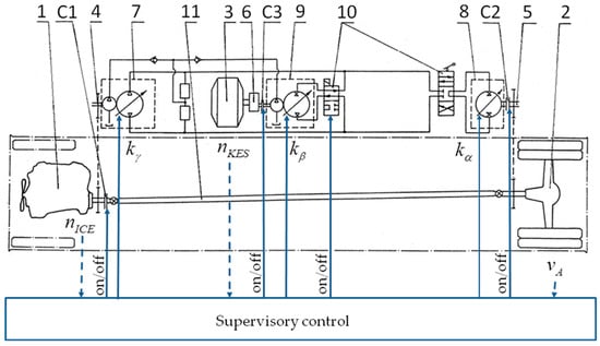
Figure 1.
A simplified scheme of the considered hybrid driveline.

Table 1.
Vehicle specification data used for simulation.
The considered structure permits following operation modes:
- -
- Primary KES charge by ICE with bus at rest, mode I;
- -
- Bus acceleration only by KES, usually used in close areas at the bus stops, mode II;
- -
- Bus deceleration by KES (recuperation mode), mode III;
- -
- KES charging by ICE during bus movement, mode IV;
- -
- Bus acceleration by ICE and KES (maximum bus dynamics), mode V;
- -
- Bus acceleration only by ICE (conventional mode);
- -
- ICE starting by KES.
3. Theoretical Model for HST Control
The main controlled object in the considered hybrid system is the HST itself, which ensures continuously variable ratios among alternative energy sources (ICE and KES) and bus drive wheels. HST control is accomplished by appropriate changes of the working displacement of the variable axial-piston hydromachines PF, PD and D according to driver requests at different modes of bus operation. A control law for HST ratio alteration must satisfy the kinematic and torque compatibility of the energy sources. The working hypothesis treats the HST inertial loads (the bus and KES) as energy sources with ‘infinitely’ large instant power. It is assumed that the HST is able to work in CPS mode at a constant pressure [29], which is influenced by the varying displacements of separate hydraulic units. The following assumptions are made: (a) HST works at a constant high pressure, except for the conventional mode; (b) ICE works at its optimum operation point and , which corresponds to the minimum specific fuel consumption; if ICE is not in use, it is switched off; (c) KES losses are modeled by KES efficiency as shown in [17]; (d) volumetric and mechanical efficiencies of the separate hydraulic units are functions of current displacement and speed of the units, as shown in Figure 2, but they are not influenced by the direction of the energy flow through the units.
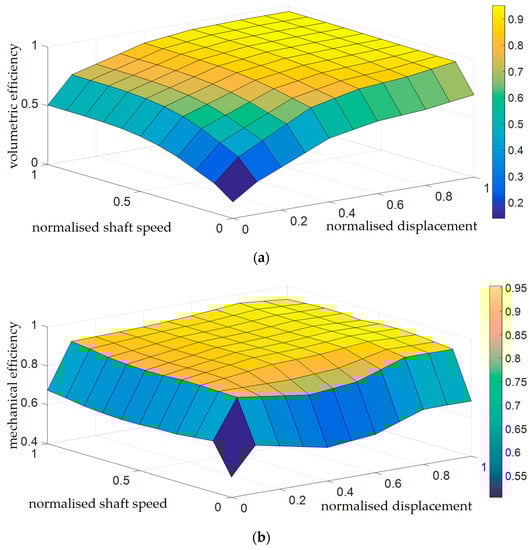
Figure 2.
Experimental data of hydromachines at : (a) Volumetric efficiency ; (b) Mechanical efficiency .
3.1. Torque Compatibility
This condition describes the relations among torques and the fluid pressure in the HST closed contour. If a working pressure value is preset, the current displacement of hydromachines D can be presented in dimensionless form as:
where depicts bus mass characteristics, describes driver requests for movement alteration, , depict air and rolling resistances acting on the bus during movement, but is the maximum tractive force, generated by the hydromachines D at the given pressure .
The torque, generated by hydromachines PF and applied to KES as a drive or load torque depending on the direction of the energy flow, is expressed by [35]
where means maximum torque, applied to KES rotor, and is the dimensionless current displacement of the hydromachines PF.
3.2. Kinematic Compatibility
The accepted working hypothesis for maintaining constant working pressure requires precise balance of flow rates, passed through the hydromachines. Taking into account the direction of flow at the aforementioned different modes of bus operation, the flow rate balance determines the flow rate, generated by the hydromachines PF, as
The flow rates are functions of current working displacement of the hydromachines, their shaft speeds and their volumetric efficiency [35], and after substituting in flow rate balance Equation (3), a kinematic relationship among kinematic parameters is obtained in the following form:
where signs “+” are related to the braking process, and signs “−“ to the acceleration process. The parameters shown in brackets indicate the corresponding speeds of the hydromachines’ shafts, taking into account the kinematic ratios of the mechanical gears. By analogy to Equations (1) and (2), the dimensionless form of the current displacement of the hydromachines PD is also included as .
From Equation (4), the KES rotor speed can be obtained as
where and are the local kinematic ratios between KES and the drive wheels and between KES and ICE, respectively, at maximum working displacements of the separate hydromachines.
3.3. Dynamic Balance and HST Control Equation
KES internal losses are the result of its own rotor motion. Two main loss contributions are usually considered: bearing losses (rolling, sliding, sealing) and air resistance (significantly reduced in vacuum), including rotor shape resistance. It is shown in [17] that the unmodeled losses can be depicted by KES efficiency, which depends on KES state of charge and applied power. If the KES angular velocity is known, usually by measurements, the KES efficiency is easily transformed as a function of its angular velocity and applied torque, as shown in Figure 3. Applying the idea for the KES efficiency the KES rotor dynamics is depicted as
where describes the internal KES losses, which for a given KES design is a function of KES angular velocity and applied torque [17].
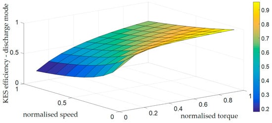
Figure 3.
KES efficiency as a function of its rotor speed and applied torque in normalized form.
The volumetric efficiency of the used hydromachines are functions of their current displacement and current speed rate, which changes over time depending on the specific bus mode of operation. If volumetric efficiency is considered as a function of time, the KES rotor acceleration can be derived from Equation (5) as
Substituting Equations (2) and (7) into Equation (6), a common HST control is obtained as
where is a maximum angular acceleration/deceleration of the KES rotor, which corresponds to the maximum torque at a given KES state of charge.
3.4. Overall Solution for HST Control Equation
It is assumed that the necessary variable ratios in the control of HST are achieved by consequent and independent alteration of working displacements of the included hydromachines. Based on this assumption, the control laws for displacement alteration in dimensionless form, i.e., , , and , are obtained for the mentioned modes of operation of the hybrid system.
The obtained form of the control Equation (8) shows that it is possible to work out the partial solutions for displacement alternation corresponding to the different modes by a linear differential equation of first order with variable coefficients in the following form
the solution of which is
where is a constant which depends on the initial conditions.
The different meanings of the coefficients and , the corresponding unknown variable and the admissible ranges of variation of the dimensionless displacements of the separate hydromachines , , and are presented in Table 2 for the different HST modes of operation. A determined value of for hydromachines PD displacement is introduced, which describes driver requests for maintaining constant acceleration or deceleration, if achievable. When ICE is used in parallel with KES modes IV and V, two values of are included. The first one describes ICE reserve of power under given conditions of bus movement. The second value corresponds to the total ICE power.
Table 2.
HST control equation coefficients and unknown variable meanings at different modes of operation of the hybrid system.
The obtained analytical solutions are used for simulations of the ICE–KES–HST system behavior when the bus follows a predefined single cycle. The cycle itself consists of an initial period of KES charge by ICE, bus fixed acceleration by using the energy stored in KES, KES charge by ICE during bus movement at constant speed, recuperation brake with constant deceleration rate, followed by an additional fixed period for further KES charge by ICE when the bus is stationary. This cycle makes it possible to determine the number of used hydromachines and the working pressure value at given acceptable durations of different modes. Kinematic parameters , , and the additive for the driver requests for acceleration or deceleration form the supervisory control inputs, and the outputs are control signals for clutches and the required displacements of the separate hydromachines, as depicted in Figure 1. The working pressure is estimated by using the Takagi-Sugeno fuzzy observer, as proposed in [36].
Assuming negligible losses in KES compared to active power applied from HST, i.e., magnetic bearings and vacuum surroundings, an illustrative example of the proposed control of the considered hybrid propulsion system and KES energy content is shown in Figure 4, where, using a quasistatic (QSS) approach [37], the hybrid bus strictly follows a typical transport cycle [38]. In the described assumptions, dimensionless displacement represents energy demands in absolute values for covering the desired bus speed profile. The dimensionless displacement represents ICE usage for keeping the overall energy level of the proposed hybrid system, if a strategy of maximum ICE usage for KES charging is adopted when the bus is at rest.
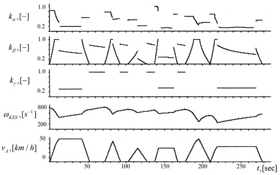
Figure 4.
Simulation results of the considered hybrid driveline: dimensionless displacements of the separate hydromachines , , and , KES energy content, described by its rotor speed , over a defined speed profile .
The energy recovery potential of the considered hybrid system is evaluated over a sequence of simple drive cycles with a speed profile consisting of acceleration and deceleration with the same intensity but with different achievable maximum speeds, as shown in Figure 5a [39]. The basic limitation here is covered mileage over the cycle, which is kept constant. The simulation process is fulfilled under the following assumptions: the acceleration process is realized on the basis of the kinetic energy stored in KES, and the ICE covers energy demands at constant speed. The ratio between recovered energy in KES during the acceleration and energy demands for acceleration, as shown in Figure 5b, describes the energy recovery potential of the proposed system. At low values of deceleration, recuperative braking is not possible, and the conventional brake system is used. The maximum value of acceleration is limited by the accepted maximum pressure in the HST and the maximum displacement of the hydromachines D. The energy recovery potential increases with increasing values of and increased intensity, i.e., higher values of acceleration/deceleration, because of more effective working ranges of the separate hydromachines at higher KES efficiency [17]. The most effective modes of operation of the considered hybrid system are and , where of the used KES energy is recuperated by KES. These results confirm the statement that the most efficient KES utilization is in the area of the most intensive vehicle dynamics, as predicted in [39].
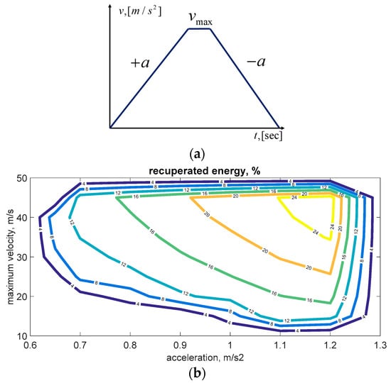
Figure 5.
Energy recovery potential over a simple drive cycle: (a) speed profile; and (b) energy recovery values. Color lines represent isolines with constant recovery potential
4. Experimental Validation of the Proposed HST Control
4.1. Test Stand Description
The idea behind the proposed control of HST and the described assumptions has to be proved in practice. A structural scheme of the created stand is shown on Figure 6a, where the components are as follows: EM-induction electric motor; A7V-variable displacement axial-piston pump A7V28LV, manufactured by Bosch-Rexroth GMBH; GM-gear motor ZM44, manufactured by Hydraulics, Bulgaria; iEM, iGM-mechanical coupling, which is the simplest variant; iKES-V-belt transmission chosen for safety reasons; KES1, KES2-two identical kinetic energy storages (Figure 6c), designed in the Department of Theory of Mechanisms and Machines, at the Technical University of Sofia. The pump A7V28LV and the motor ZM44 create the stand HST, which allows bidirectional energy transfer at a reasonable simplicity and price. The considered structural scheme is very similar to the diagram proposed in [40], but the attention here is directed at the control of the variable displacement of axial-piston pump A7V28LV. The component parameters are listed in Table 3.
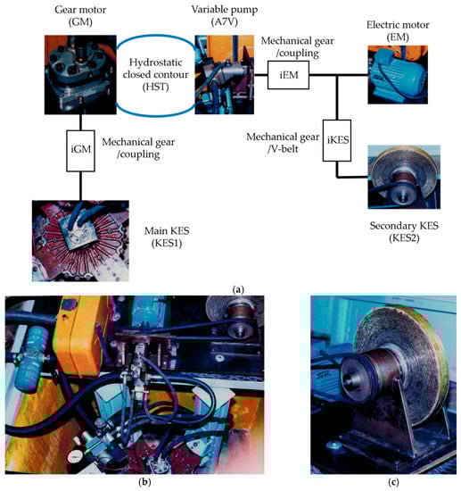
Figure 6.
Test stand for HST control validation. (a) Structural scheme: straight lines represent mechanical links; curved lines, hydraulic links; (b) test stand view; and (c) winded KES rotor technology.
Table 3.
Test stand components characteristics.
Two operational modes are available. In regime A, which corresponds to the KES charging mode of the hybrid system, the electric motor EM charges the main KES through stand HST, where the variable displacement pump A7V ensures the necessary variable ratio between the electric motor and KES1. During the second regime B, the energy, stored in the main KES1, is transferred back to the electric motor. The electric motor is switched off and it is used as an inertia load of the HST. The pump A7V, which works as a motor, realizes the necessary variable ratio between both inertia loads. The second KES2 is used as an additional inertia load for HST, and corresponds to the vehicle inertial load. This regime corresponds to bus acceleration only by KES.
4.2. Mathematical Model of Stand HST Control System
For the purposes of this investigation, the control system of the variable displacement pump A7M is redesigned. The hydraulic scheme of the suggested test stand and the hydro-mechanical scheme of the new control system of the variable pump A7V are shown in Figure 7. The elements labelled on Figure 7 are: 1—variable pump A7V28LV; 2—constant gear motor ZM44; 3—main kinetic energy storage KES1; 4—secondary kinetic energy storage KES2; 5—electric motor; 6—V-belt mechanical couplings; 7—control valve; 8—directional valve, type PX06; 9—directional valve, type PX10; 10—control cylinder of the pump A7V; 11—restrictor; 12—restrictor; 13—relief valve, type A3A3; 14—oil filter; 15—control piston of the pump A7V; 16—control valve spool; 17—the spool of the directional valve PX06.

Figure 7.
Proposed schemes of the test stand. (a) Hydraulic scheme of the stand; and (b) hydro-mechanical scheme of the A7V pump control system.
4.3. Working Hypothesis and Assumptions
The following assumptions are made for solving the investigation problem of the study of the considered control system: (a) the working fluid is compressible; (b) the fluid friction forces are proportional to the velocities of the moving spool and the piston; (c) the restrictor, labelled as 12 on Figure 7, affects the control system by nonlinear resistance force on the spool 16; (d) impact effects are considered because of the limited spool and piston displacements; (e) energy losses in KES1 and in the electric motor EM are neglected; (f) electric motor characteristic is modelled as a 4th order polynomial of its rotor speed; (g) average constant efficiencies of the separate hydromachines are accepted; (h) all friction forces, except the aforesaid, are neglected, their influence is partially described by hydro-mechanical efficiency of the hydromachines.
4.4. Mathematical Model
Interactions between the inertia loads at the given control system, taking into account the assumptions mentioned above, is depicted by the following system
Different coefficients are used for description of the stand modes of operation and corresponding conditions of separate hydromachines:
- regime A: : : ;
- regime B: : : ; .
The dynamic equivalence method between the hybrid driveline parameters and the test stand ones is used to evaluate the equivalent working pressure in the stand HST, the EM nominal power, and the KES1 and KES2 moments of inertia. As some of the parameters above are given in advance, for example, time scale factors for both regimes are evaluated. Detailed description of the used parameters and the model derivation are given in Appendix A.
5. Results from Mathematical Modelling Compared with Experimental Results
5.1. Experiment Description
Just one sequence of available modes is considered here. Initially the electric motor EM (5) is used to accelerate the secondary KES2 (4) via V-belt coupling (6) till stable speeds are achieved. During this period the pressure relief valve (13) is kept fully open, thus separating the pump A7V (1) from the EM as the whole pump flow passes to the tank (T). The first main mode of the test stand operation, considered as regime A and shown in Figure 8, coincides with mode I (KES charge by ICE) of the bus hybrid system, and this mode starts on when the relief valve (13) is activated remotely to its preset. The pump A7V (1) works as a pump and through the gear motor ZM44 (2) accelerates the main KES1 (3). The duration of the process is defined in advance by the operator until stable speeds are achieved. There are almost no variations of the EM and the A7V common shaft speed because of the additional inertial mass of the secondary KES2 (4).
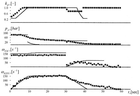
Figure 8.
Comparative analysis results: approximate theoretical model—solid line; experimental data—“*”.
The test stand design requires KES2 (4) deceleration with EM (5) switched off, as the used pump A7V (1) is intended for open hydrostatic contour. The pressure relief valve (13) is kept fully open during this mode. This defines the zero speed of at the beginning of the second main mode as it is shown on Figure 8. The directional valve (9) is switched accordingly to reverse the fluid flow, and the second main stand mode starts with remote activation of the relief valve (13). The energy now flows from the main KES (3), the gear motor ZM44, which works in pump mode, the pump A7V, which works in motor mode, and the secondary KES2 (4) accelerates on the account of the energy stored in KES1 (3). If the main KES1 (3) is considered to be equivalent to inertial bus mass and the secondary KES2 (4) is equivalent to the KES from the bus hybrid system, this main mode, designated as regime B, coincides with mode III (bus deceleration by KES, as it is described in Section 2) with a constant bus acceleration, determined by the constant volume of the motor ZM44 (2). The duration of the process is determined by the dissipation of the entire energy, stored in the KES.
5.2. Results Comparison
Obtained experimental data are compared in Figure 8 with the results of a simplified theoretical model. This model consists of the last two equations of the system (11), which describe the inertial loads behavior. The first regime (regime A) has a duration of 30 s until the KES1 reaches its stable speed, which is defined by EM speed and HST ratio at maximum displacement of the pump A7V (1). Three stages of the process are clearly distinguished. The first stage, with duration of approximately 4 s, corresponds to HST mode of maximum pressure with open relief valve. The pump A7V (1) works with minimum displacement, and as the ZM44 displacement is constant, this leads to almost constant maximum acceleration of KES1 (3). The second stage corresponds to the considered strategy of HST control at a constant working pressure. This constant pressure is achieved by increasing of the variable displacement of the pump A7V (1), increasing values of the coefficient . Over those two stages, the EM speed is almost a constant. The third stage describes the energy transfer at constant displacements of both hydromachines A7V (1) and ZM44 (2), but with increased EM speed. In fact, the real process proceeds more quickly due to the unmodeled mechanical and hydraulic losses. The constant value of the working pressure gives an idea of the level of those losses.
The second regime starts at 30 s and has a duration of another 30 s until the HST working pressure drops to zero. The beginning of the process is connected to preliminary increasing of the working pressure, which is determined by the inertia load of the masses, KES2 (4), connected to the EM shaft. This pressure, according to the control algorithm and the designed control scheme of A7V (1), specifies the balanced working displacement of the pump A7V (1). The used dynamic equivalence method determines very low equivalent working pressure, just around 25 bars, which corresponds to lower limit of stable working mode of the stand HST. The working pressure in HST is defined by the resistances on EM shaft and on the KES2 (4) respectively. The summarized inertia load defines the duration of the process of energy transfer. The HST control process lasts 12 s at almost constant displacements of both hydromachines.
6. Conclusions
The generalized control law for the HST ratio for a hybrid drive line including KES with CPS is obtained. Choosing appropriate control variables, partial solutions of the HST control law are depicted, depending on different driving modes and driver requests. The energy recovery maximum potential is estimated around 20–25% over a simple drive cycle. A simple experimental scenario is carried out which confirms the basic idea for controlling the HST in the bus hybrid system when KES is used as an energy storage. The presented theoretical model is suitable for modelling the energy transfer process in such hybrid drive lines over different speed profiles and different vehicle modes of operation. The KES losses, simulated by KES efficiency coefficient, can be compensated by using KES speed data. The whole process of energy transfer in different modes of operation will be fulfilled, if variable displacement hydromachines with Solenoid Control Electronic Swashplate with Position Sensor, available from Bosch-Rexroth GMBH or Eaton Corp., are used to form HST contour.
Author Contributions
Conceptualization by V.J. and V.D.; experiment design and experimental data collection by V.D.; data analysis by V.J. and V.D.
Funding
The APC was funded by project BG05M2OP001-1.001-0008 “National Center for Mechatronics and Clean Technologies” Operational Programme Executive Agency, Ministry of Education and Science, Bulgaria.
Conflicts of Interest
The authors declare no conflict of interest.
Appendix A
Mathematical model of the test stand—a detailed description.
Table A1.
The list of variables, describing the test stand dynamic behavior, Equation (11) in the main text.
Table A1.
The list of variables, describing the test stand dynamic behavior, Equation (11) in the main text.
| Nomenclature | |
|---|---|
| angular speed of the shaft of the electric motor EM (5) | |
| angular speed of the rotor of the main KES1 (3) | |
| control fluid pressure in the chamber of the cylinder (10) | |
| dimensionless current displacement of the pump A7V (1) * | |
| position of the spool plunger (16) | |
| position of the piston (16) * | |
| working fluid pressure in HST contour |
* There is a known linear dependency between the two variables.
Table A2.
The list of used parameters.
Table A2.
The list of used parameters.
| Parameter | Value or Range |
|---|---|
| coefficient of linear resistance spool plunger (16) * | |
| coefficient of non-linear resistance spool plunger (16) * | |
| coefficient of linear resistance control piston (15) * | |
| coefficient of the control valve flow | |
| coefficient of the restrictor (11) flow | |
| coefficient of pressure relief valve (13) * | |
| control cylinder stroke | |
| control spring constant | |
| control valve spool stroke | |
| cross-sectional areas of the piston | , |
| cross-sectional area of the spool plunger | |
| diameter of the flow section of the control valve | |
| electric motor empirical coefficients | |
| electric motor nominal torque/speed | / |
| equivalent mass moment of inertia at A7V | |
| equivalent mass moment of inertia at ZM44 | |
| flow section of the restrictor (11) * | |
| fluid density | |
| fluid elastic modulus | |
| kinematic viscosity of the fluid | |
| mass of the piston (15) | |
| mass of the spool plunger (16) | |
| maximum flow section of the control valve (7) * | |
| maximum fluid pressure | |
| maximum spring force | |
| spring constant | |
| volume of the HST contour |
* This parameter is considered to be a varying parameter in simulations.
The six variables, given in AA1, describe the test stand dynamic behavior, the principal scheme of which is shown in Figure 7. The position of the spool plunger (16) of the control valve (7) determines the control fluid pressure in the chamber of the control cylinder (10). The pressure balance over the control piston (15) specifies its position , which directly relates to the current displacement of the variable pump A7V (1), which, taking into account the mechanical gear ratios () determines the necessary variable ratio between angular speeds of the electric motor (5) shaft— and the main KES1 (3) rotor—. By analogy, this displacement is considered in dimensionless form as .
Two active forces, two hydraulic resistance ones, and geometric limitation are considered regarding to the motion of the spool plunger (16). The active forces are a hydraulic one caused by working fluid pressure in the hydrostatic transmission (HST) contour
and a linear spring force
where parameter defines mechanical connection between the spool plunger (16) and the spring (, or otherwise . This structural change happens at a specific spool plunger position , determined by the control system design.
According to the assumptions, the hydraulic resistances created during the movement of the spool plunger (16) can be presented as a function of the spool plunger velocity .
Coefficients of the resistance and are calculated by [41]:
where are the spool plunger diameter and guide length, , is the spool diameter clearance, , is a flow sectional area of the restrictor (12), , but is a coefficient of flow through the restrictor (12).
If the spool plunger (16) reaches its left end position with some velocity of , an impact occurs between the spool plunger (16) and the control valve housing. This impact is considered as reaction in the following form
where is the velocity restitution coefficient, is the impact duration, , and parameter describes the impact existence (), or otherwise .
Combining relations (A1) through (A5) into the equation of the spool plunger rectilinear motion, the following expression is obtained
The current position of control piston (15) is determined by the balance of three active forces, two opposite forces caused by pressures and one spring force, which by analogy with relations (A1) and (A2) can be presented as
where is the maximum possible spring force, , is the control piston (15), which corresponds to the minimum displacement of the pump A7V (1).
Only linear hydraulic resistance is considered here, which has two components related to the different guides of the control piston (7)
where equivalent coefficient of resistance is calculated by [41]
The piston movement is limited by the pump A7V design. If the control piston (7) reaches its final positions and , corresponding to the minimum and the maximum displacement of the pump A7V (1) impact effects occur between the piston and the pump housing. Taking into account the necessary conditions for impact existence, the respective impact reactions are
where, by analogy with (A5), the parameters describe the impact existence (), or otherwise , and ), or otherwise , respectively.
Substituting the relations (A8) through (A10) into the equation of rectilinear motion of the control piston (15) and considering the direction of the separate forces, the equation of the control piston movement is as follows:
Equation (A11) describes the control piston displacement, and by a coefficient of proportionality, this solution describes the current working displacement of the variable pump A7A (1).
The equilibrium of the active forces on the control piston (15), which defines the pump A7V displacement, is determined by a control pressure at the constant value of the working pressure in the HST contour. This control pressure depends on the flow rates to and from the chamber of the control cylinder (10), and on the momentary chamber volume. The differential equation for the control pressure variance is
where the expression in the denominator describes the current volume of the chamber at the piston position , , , and are the flow rates through the control valve (7), through the restrictor (11), and the flow rate caused by the piston movement, respectively.
The flow rate depends on the position of the spool (16) of the control valve (7) and on the position of the directional valve (8). The flow rate direction and value are determined by the difference between the pressure , and the working pressure or between the pressure and the low pressure in the tank (T). Combining these conditions leads to
where is the middle position of the spool (16) with no flow rates through the control valve (7), and parameters , which identify only positive flow rates, depending on the test stand regimes:
- regime A—energy transfer from the pump A7V (1) to the gear motor ZM44 (2):
- regime B—energy transfer from the gear motor ZM44 (2) to the pump A7V (1):
The flow rate is a flow rate through the restrictor (11) and its value can be calculated by [41]:
The last flow rate is caused from the displacement of the piston (15) and can be calculated by the relation (41):
Substituting separate flow rate relations (Equations (A13)–(A15)) into Equation (A12) and making some arrangements, the equation which describes the variance of the control pressure is
The working pressure depends on the balance of the flow rates in HST contour. As the volume of the HST contour is approximately constant the differential equation for the working pressure variance is
where parameter depends on the test stand regime. If the energy transfer is from the pump A7V (1) to the gear motor ZM44 (2), i.e., regime A, is positive, ; if the energy transfer is in the opposite direction, i.e., regime B, is negative, . Parameter describes the condition when the working pressure rises above the preset maximum pressure and switches from to .
The flow rates of the variable pump A7V (1) and the gear motor ZM44 (2), and respectively, can be expressed by
The flow rate through the pressure relief valve (13) is [41]
and this flow rate exists only if the working pressure , i.e., .
After substituting the relations (Equations (A18) and (A19)) into Equation (A17) and making some transformations, the final form of the working pressure equation is obtained as
where means the kinematic ratio between the electric motor (5) and the main KES1 (3) at maximum displacement of the pump A7V (1) with accuracy to the volumetric efficiencies of the pump A7V (1) and the motor ZM44 (2).
The equation of motion of the electric motor shaft can be presented as [42]
where the electric motor torque is approximated by [43]
and the torque generated by the pump A7V (1) is expressed by
The parameters and define the direction of the energy flow, i.e., the two regimes A and B of the test stand: during regime A, and during regime B, .
Substituting relations (Equations (A22) and (A23)) into Equation (A21), the equation of the shaft of the electric motor EM (5) becomes
By analogy with Equation (A21), the equation of the main KES1 (3) can be written in the following form [42]
where the parameter has already been defined and the torque of the gear motor ZM44 (2) has a similar form as presented by (Equation (A23)), i.e.,
After substituting relation (Equation (A26)) into Equation (A25), the equation of the main KES1 (3) is as follows
The system, combining Equations (A6), (A11), (A16), (A20), (A24) and (A27), represents the dynamic behavior of the test stand.
References
- Vazquez, S.; Lukic, S.; Galvan, E.; Franquelo, L.G.; Carrasco, J.M.; Leon, J.I. Recent advances on energy storage systems. In Proceedings of the IECON 2011—37th Annual Conference on IEEE Industrial Electronics Society, Melbourne, Australia, 7–10 November 2011. [Google Scholar]
- Copex, J.P. Le gyrobus d’Yverdon fête ses 50 ans. Tram. Mag. 2003, 76, 34–46. (In French) [Google Scholar]
- Dhand, A.; Pullen, K.R. Review of flywheel based internal combustion engine hybrid vehicles. Int. J. Automot. 2013, 14, 797–804. [Google Scholar] [CrossRef]
- Greenwood, C.; Brockbank, C. Formula 1 Mechanical Hybrid Applied to Mainstream Automotive. Available online: www.torotrak.com/Resources/Torotrak/VDI_2008.pdf (accessed on 17 August 2018).
- Jaguar’s Advanced XF ‘Flybrid’. 2010. Available online: https://www.autocar.co.uk/car-news/concept-cars/jaguars-advanced-xf-flybrid (accessed on 29 June 2018).
- Howard, B. Volvo Hybrid Drive: 60000 Rpm Flywheel, 25% Boost to Mpg. 2013. Available online: https://www.extremetech.com/extreme/154405–volvo–hybrid-drive-60000-rpm-flywheel-25-boost-to-mpg (accessed on 29 June 2018).
- Doucette, R.T.; McCulloch, M.D. A comparison of high-speed flywheels, batteries, and ultracapacitors on the bases of cost and fuel economy as the energy storage system in a fuel cell based hybrid electric vehicle. J. Power Sources 2011, 196, 1163–1170. [Google Scholar] [CrossRef]
- Hedlund, M.; Lundin, J.; Santiago, J.; Abrahamsson, J.; Bernhoff, H. Flywheel energy storage for automotive applications. Energies 2015, 8, 10636–10663. [Google Scholar] [CrossRef]
- Tupen, A. Tesla Semi Truck’s Battery Pack and Overall Weight Explored. 2018. Available online: https://www.teslarati.com/how-much-tesla-semi-truck-battery-pack-weigh (accessed on 29 June 2018).
- Klevenfield, F. Premiere for Volvo Trucks’ First All-Electric Truck. 2018. Available online: https://www.volvogroup.com/en-en/news/2018/apr/news-2879838.html (accessed on 29 June 2018).
- Read, M.G.; Smith, R.A.; Pullen, K.R. Optimisation of flywheel energy storage systems with geared transmission for hybrid vehicles. J. Mech. Mach. Theory 2015, 87, 191–209. [Google Scholar] [CrossRef]
- Beachley, N.H.; Frank, A.A. Continuously Variable Transmissions: Theory and Practice. 1979. Available online: https://www.osti.gov/servlets/purl/5529813 (accessed on 29 June 2018).
- Schilke, N.A.; DeHart, A.O.; Hewko, L.O.; Matthews, C.C.; Pozniak, D.J.; Rohde, S.M. The design of an engine-flywheel hybrid drive system for passenger cars. J. Automob. Eng. 1986, 200. [Google Scholar] [CrossRef]
- Igor, T. Comparative Analysis of Alternative Hybrid Systems for Automotive Applications. Ph.D. Thesis, University of Bologna, Bologna, Italy, 2012. [Google Scholar]
- Owano, N. “Flybus” Prototype May Be Hybrid Bus of Future. 2011. Available online: https://phys.org/news/2011-09-flybus-prototype-hybrid-bus-future.html (accessed on 29 June 2018).
- F1 Fuel-Saving Flywheel to Be Fitted to London’s Buses. 2012. Available online: https://www.theguardian.com/environment/2012/apr/18/f1-fuel-saving-flywheel-buses (accessed on 29 June 2018).
- Jivkov, V.; Draganov, V. The kinetic energy storage as an energy buffer for electric vehicles. Adv. Automob. Eng. 2017, 6. [Google Scholar] [CrossRef]
- Zeng, X.; Wang, J. Analysis and Design of the Power-Split Device for Hybrid Systems; Beijing Institute of Technology Press: Beijing, China; Springer Nature: Singapore, 2018. [Google Scholar]
- Dhand, A.; Pullen, K. Analysis of continuously variable transmission for flywheel energy storage systems in vehicular application. J. Mech. Eng. Sci. 2015, 229, 273–290. [Google Scholar] [CrossRef]
- Shen, S.; Veldpaus, F.E. Analysis and control of a flywheel hybrid vehicular powertrain. IEEE Trans. Control Syst. Technol. 2004, 12, 645–660. [Google Scholar] [CrossRef]
- Diego-Ayala, U.; Martinez-Gonzalez, P.; McGlashan, N.R.; Pullen, K.R. The mechanical hybrid vehicle: An investigation of a flywheel-based vehicular regenerative energy capture system. J. Automob. Eng. 2008, 222, 2087–2101. [Google Scholar] [CrossRef]
- Hagin, F.; Martin, S.; Zelinka, R. Use of hydrostatic braking and flywheels systems in buses (hydrobus and gyrobus): Their future applications in hybrid electric vehicle to reduce energy consumption, and to increase range and performance. In Proceedings of the Electric Vehicle Development Group (EVDG) 4th International Conference: Hybrid, Dual Mode and Tracked Systems, London, UK, 1981. Available online: https://trid.trb.org/view/218840 (accessed on 17 August 2018).
- Tripathy, S.C. Simulation of flywheel storage system for city bus. Energy Convers. Manag. 1992, 33, 243–250. [Google Scholar] [CrossRef]
- Lindzus, E. HRB-Hydrostatic Regenerative Braking System: The Hydraulic Hybrid Drive from Bosch Rexroth. 2008. Available online: https://www.iswa.org/uploads/tx_iswaknowledgebase/Lindzus.pdf (accessed on 30 June 2018).
- Hydraulic Launch Assists the Eaton HLA System. 2008. Available online: www.etopiamedia.net/mtw/pdfs/EatonHLA1.ppt (accessed on 30 June 2018).
- Rydberg, K. Energy Efficient Hydraulic Hybrid Drives. Available online: www.diva-portal.org/smash/get/diva2:373607/FULLTEXT01.pdf (accessed on 30 June 2018).
- Ho, T.; Ahn, K. Modeling and simulation of hydrostatic transmission system with energy regeneration using hydraulic accumulator. J. Mech. Sci. Technol. 2010, 24, 1163–1175. [Google Scholar] [CrossRef]
- Van de Ven, J.D. Increasing hydraulic energy storage capacity: Flywheel-accumulator. Int. Soc. Fluid Power 2009, 10, 41–50. [Google Scholar] [CrossRef]
- Nakazawa, H.; Yokota, S.; Kita, Y. A hydraulic constant pressure drive system for engine-flywheel hybrid vehicles. Proc. JFPS Int. Symp. Fluid Power 1996, 1996, 513–518. [Google Scholar] [CrossRef]
- Re, L. Nonlinear modeling and black-box identification of a hydrostatic transmission for control system design. Math. Comput. Model. 1990, 14, 219–224. [Google Scholar]
- Kugi, A.; Schlacher, K.; Aitzetmüller, H.; Hirmann, G. Modeling and simulation of a hydrostatic transmission with variable-displacement pump. Math. Comput. Simul. 2000, 53, 409–414. [Google Scholar] [CrossRef]
- Filipi, Z.; Kim, Y.J. Hydraulic hybrid propulsion for heavy vehicles: Combining the simulation and engine-in-the-loop techniques to maximize the fuel economy and emission benefits. Oil Gas Sci. Technol. 2010, 65, 155–178. [Google Scholar] [CrossRef]
- Deppen, T.O.; Alleyne, A.G.; Stelson, K.; Meyer, J. A model predictive control approach for a parallel hydraulic hybrid powertrain. In Proceedings of the 2011 American Control Conference, San Francisco, CA, USA, 29 June–1 July 2011. [Google Scholar]
- Ramakrishnan, R.; Hiremath, S.S.; Singaperumal, M. Dynamic analysis and design optimization of series hydraulic hybrid system through power bond graph approach. Int. J. Veh. Technol. 2014, 2014. [Google Scholar] [CrossRef]
- Costa, G.; Sepehri, N. Hydrostatic Transmissions and Actuators; John Wiley & Sons: Hoboken, NJ, USA, 2015. [Google Scholar]
- Schulte, H.; Gerland, P. Observer design using T-S fuzzy systems for pressure estimation in hydrostatic transmissions. In Proceedings of the 2009 Ninth International Conference on Intelligent Systems Design and Applications, Pisa, Italy, 30 November–2 December 2009. [Google Scholar]
- Guzzella, L.; Sciarretta, A. Vehicle Propulsion Systems, Introduction to Modelling and Optimization, 2nd ed.; Springer: Berlin, Germany, 2007. [Google Scholar]
- Regar, K.; Schneider, B. Systemanalyse und experiment—Die entwicklung eines hocheffizient antriebssytems mit brems-energie-ruckgewinnung. ATZ Automobiltechnische Zeitschrift 1985, 87, 351–358. (In German) [Google Scholar]
- Jivkov, V.; Draganov, V.; Stoyanova, Y. Energy recovery coefficient and its impact on achievable mileage of an electric vehicle with hybrid propulsion system with kinetic energy storage. Int. J. Mech. Eng. Autom. 2015, 2. [Google Scholar] [CrossRef]
- Yang, X. Experimental research of a flywheel hybrid vehicle, advanced materials research. Adv. Mater. Res. 2012, 479–481, 439–442. [Google Scholar]
- Grozev, G.; Obretenov, V.; Lazarov, M. Hydraulic Machines; Technika: Sofia, Bulgaria, 1994. (In Bulgarian) [Google Scholar]
- Minchev, N.; Jivkov, V.; Enchev, K.; Stoyanov, P. Theory of Mechanisms and Machines; Softtrade: Sofia, Bulgaria, 2011. (In Bulgarian) [Google Scholar]
- Andonov, A.; Jivkov, V.; Pavlov, S. Mechanical Elements and Mechanisms; Technical University of Sofia: Sofia, Bulgaria, 2004. (In Bulgarian) [Google Scholar]
© 2018 by the authors. Licensee MDPI, Basel, Switzerland. This article is an open access article distributed under the terms and conditions of the Creative Commons Attribution (CC BY) license (http://creativecommons.org/licenses/by/4.0/).