Design of a Ventilation System Coupled with a Horizontal Air-Ground Heat Exchanger (HAGHE) for a Residential Building in a Warm Climate


Abstract
Highlights
- -
- The ventilation system of a residential building is investigated in a warm climate.
- -
- The design of a Horizontal Air-Ground Heat Exchanger is optimized.
- -
- Different HAGHE configurations have been modelled and compared.
- -
- The operative air temperature (TOP) has been evaluated inside the building.
- -
- The optimized HAGHE system assures a proper indoor ventilation.
1. Introduction
1.1. Building Optimal Design in a Warm Climate
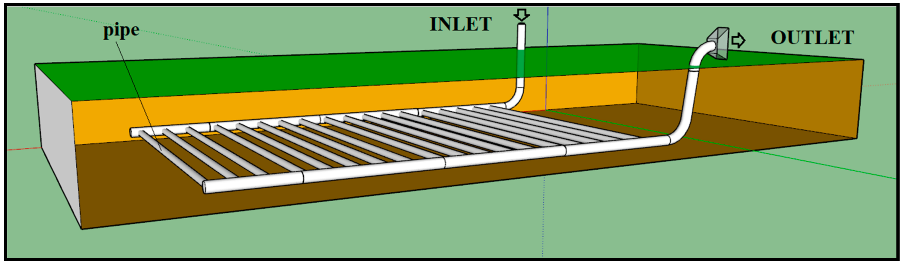
1.2. Horizontal Air-Ground Heat Exchangers (HAGHEs)
2. Methodology
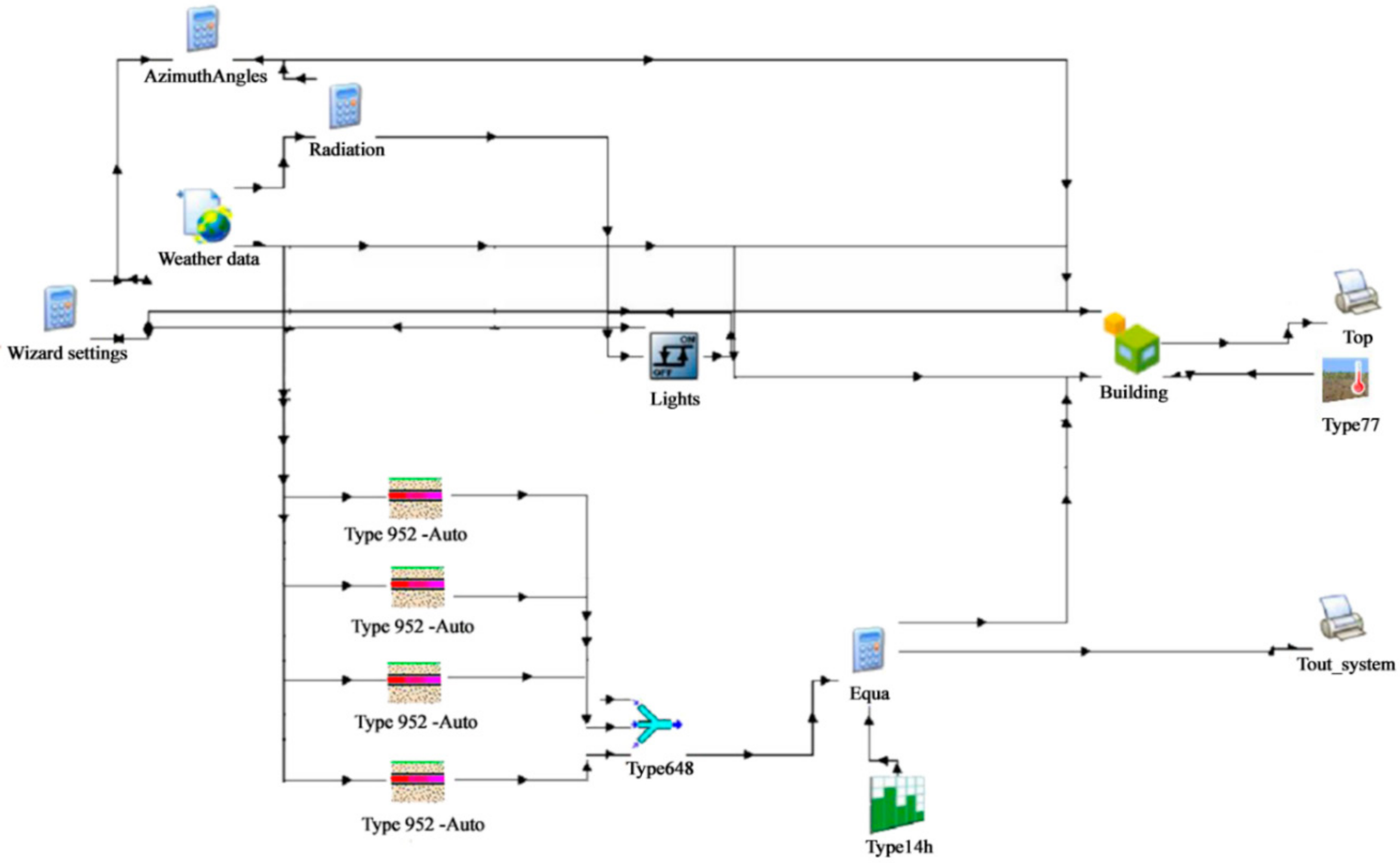
2.1. The Building Modeling
- Building information on envelope, walls, stratigraphy, materials, floor, roof, windows, and thermal loads (Type 56);
- Soil characteristics (Type 77);
- Weather data (Type 15) including the weather data of the location (data generated by Meteonorm);
- Single Pipe System in GHP (Geothermal Heat Pump) Library (Type 952);
- Time forcing function, varying from 0 (system turned off) to 1 (system turned on) (Type 14h).
- “Mean surface temperature” is the mean temperature of the air at zero altitude;
- “Amplitude of surface temperature” indicates the difference between the maximum temperature and the mean temperature (related to the temperature of the air at zero altitude);
- “Time shift” is the difference between the first day of the year and the day when there is the lowest annual temperature in a specific location.
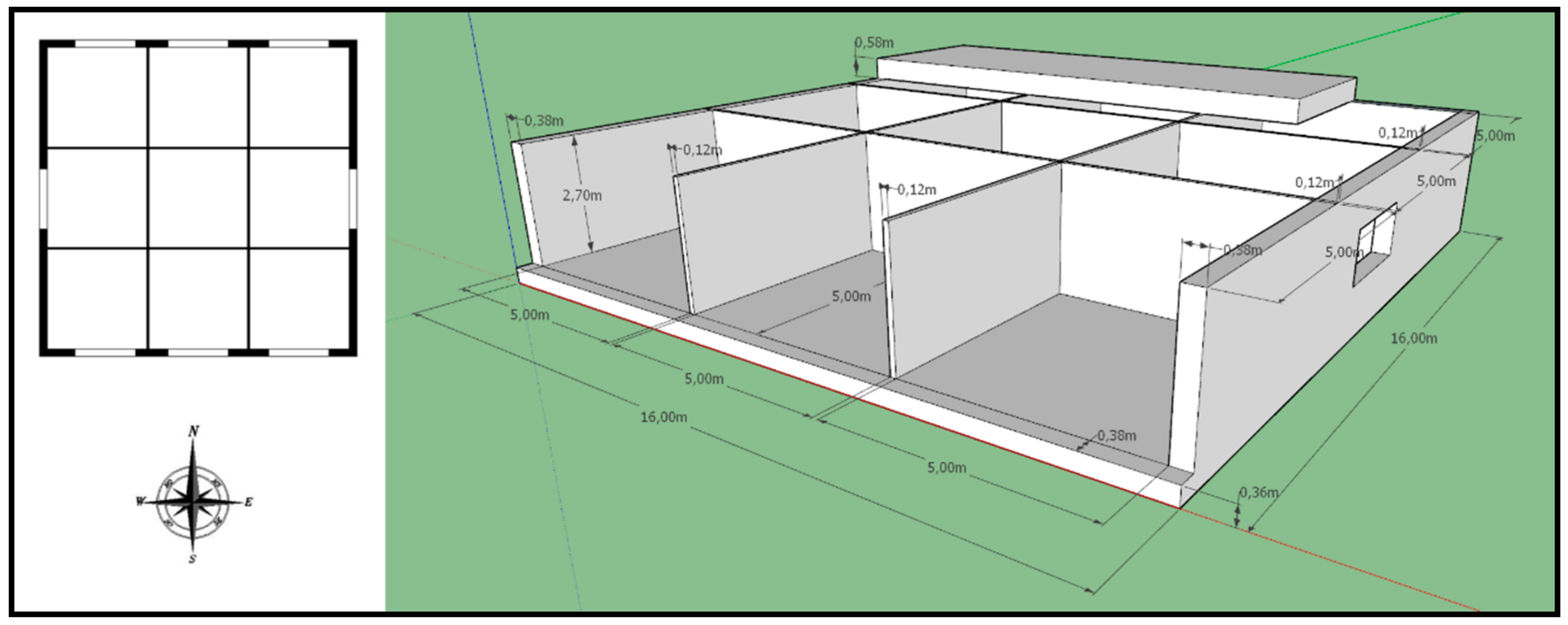
2.2. The Case Study
2.3. The Calculation Method
3. Results and Discussion
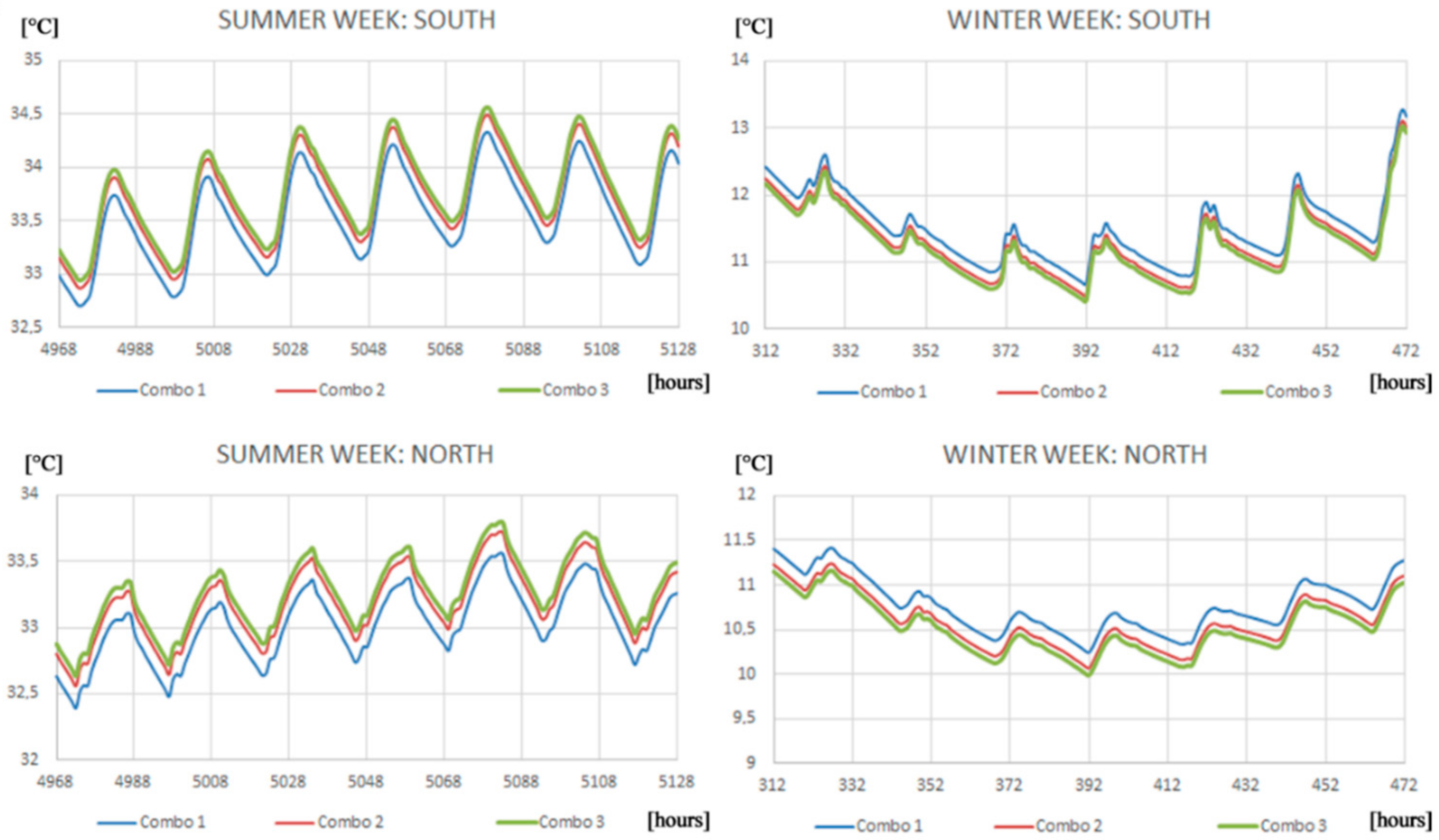
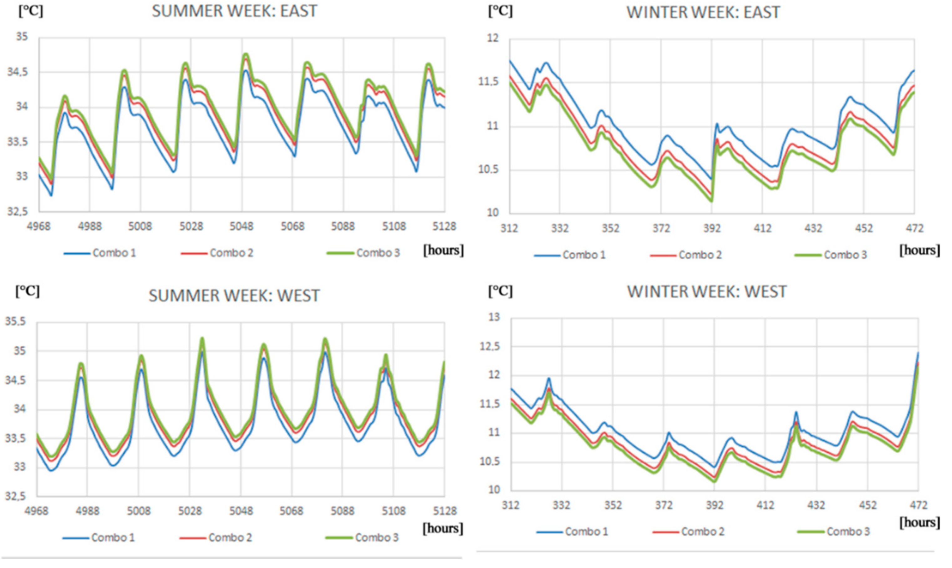
3.1. The First Step: Different Ground Thermal Conductivity Evaluation (No Geothermal System)
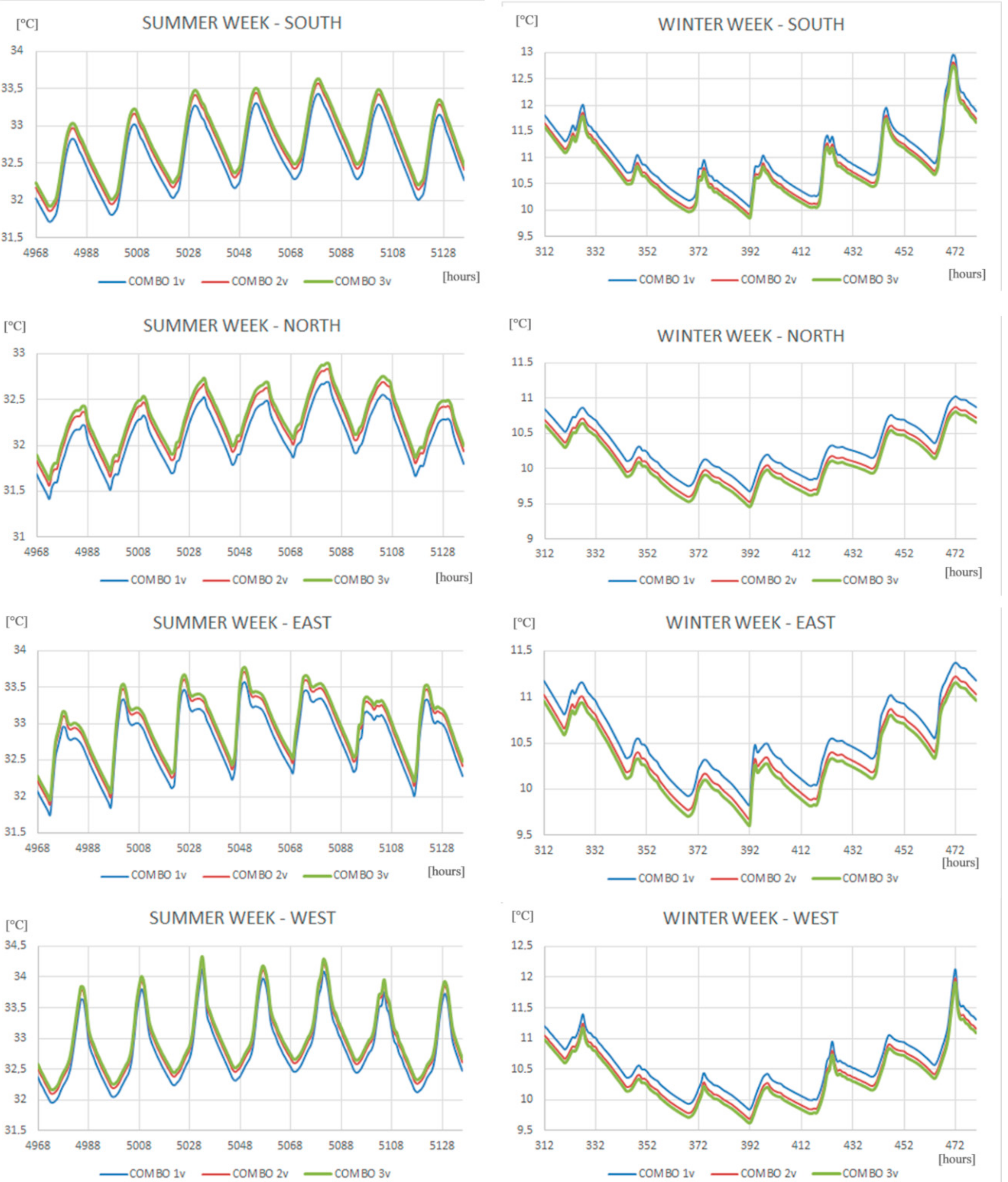
3.2. The Second Step: Natural Ventilation with Different Ground Thermal Conductivities (No Geothermal System)
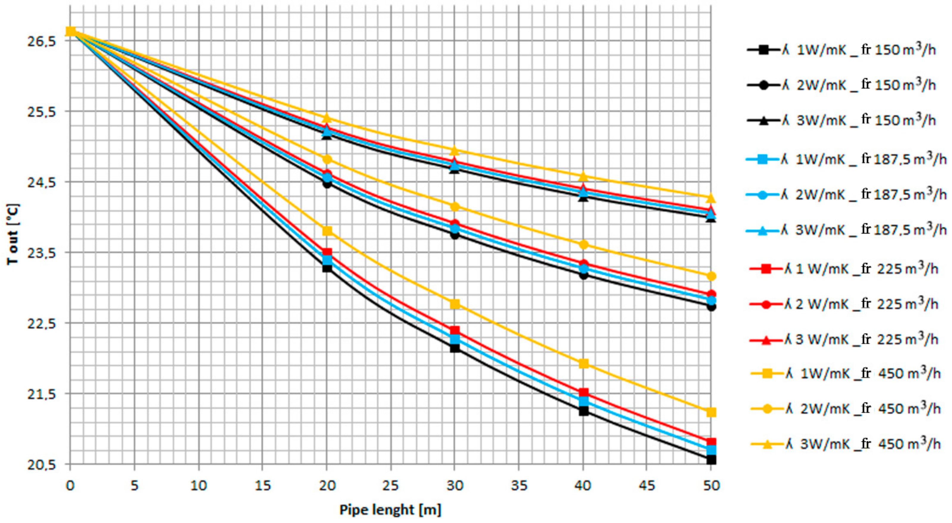
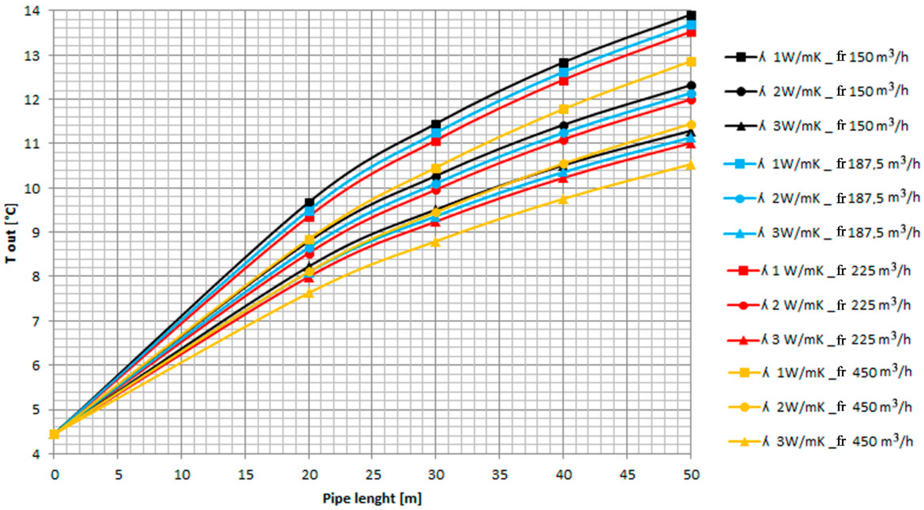
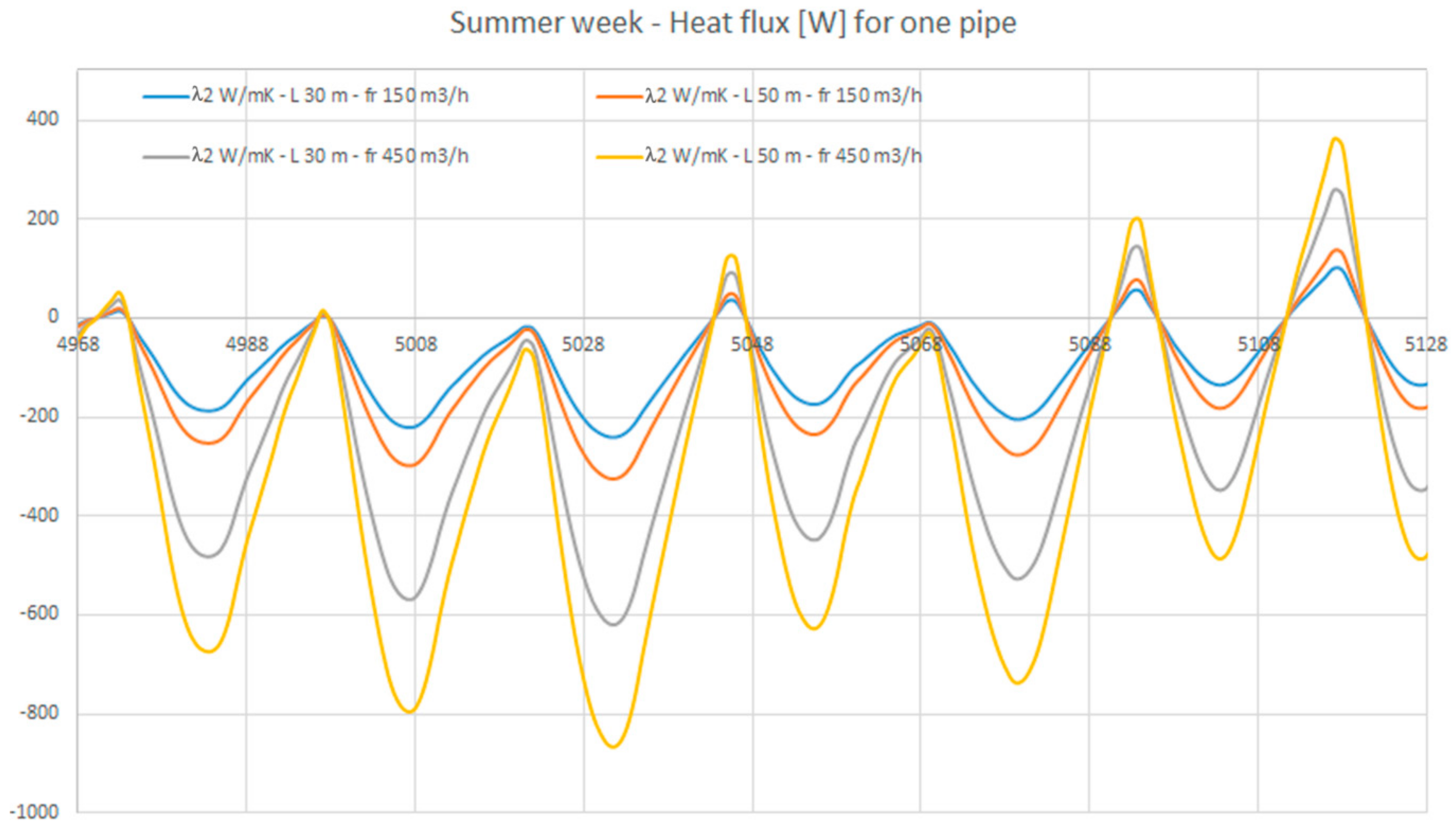
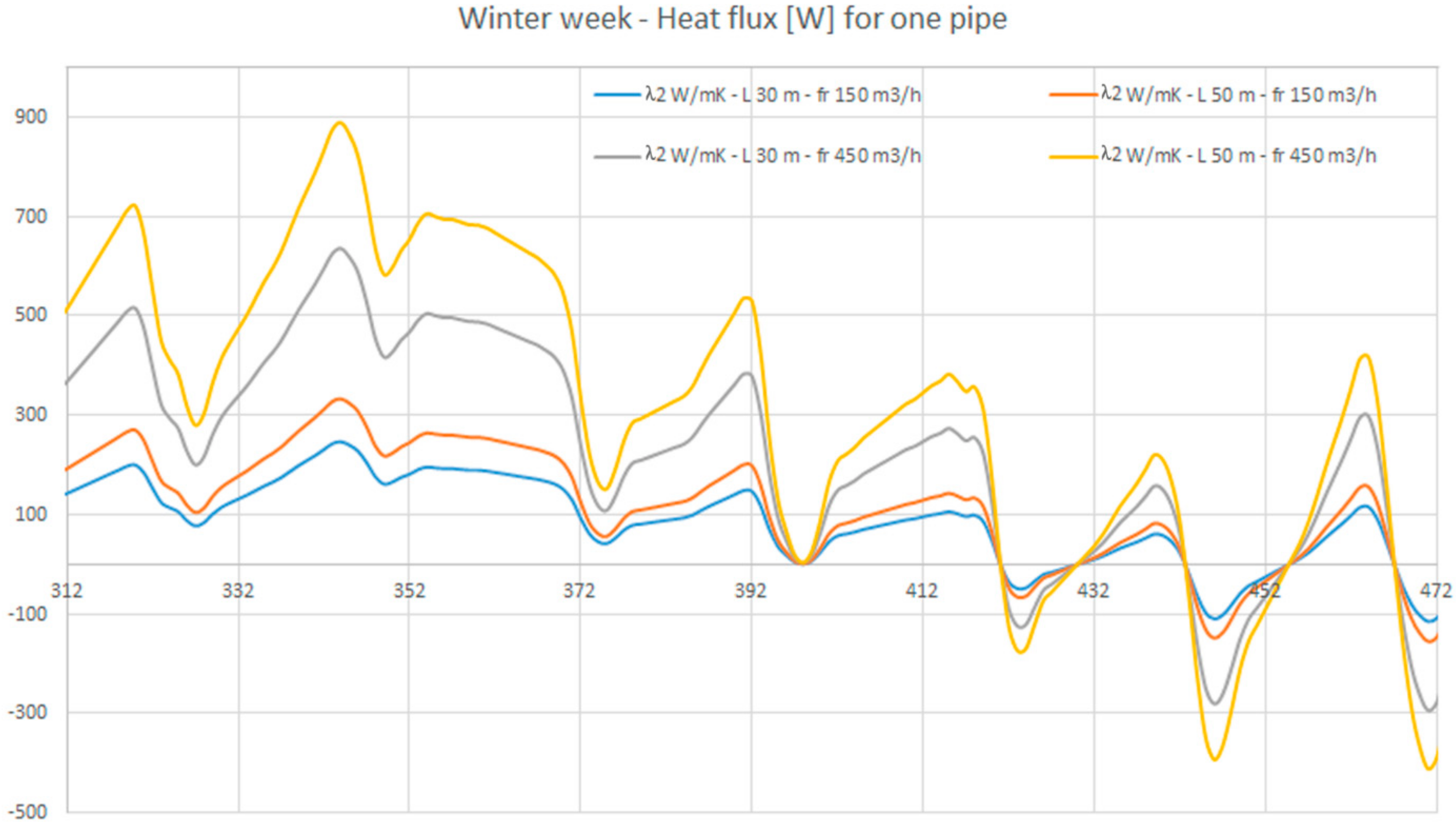
3.3. The Third Step: Analysis of Different Single Pipe Flow Rates
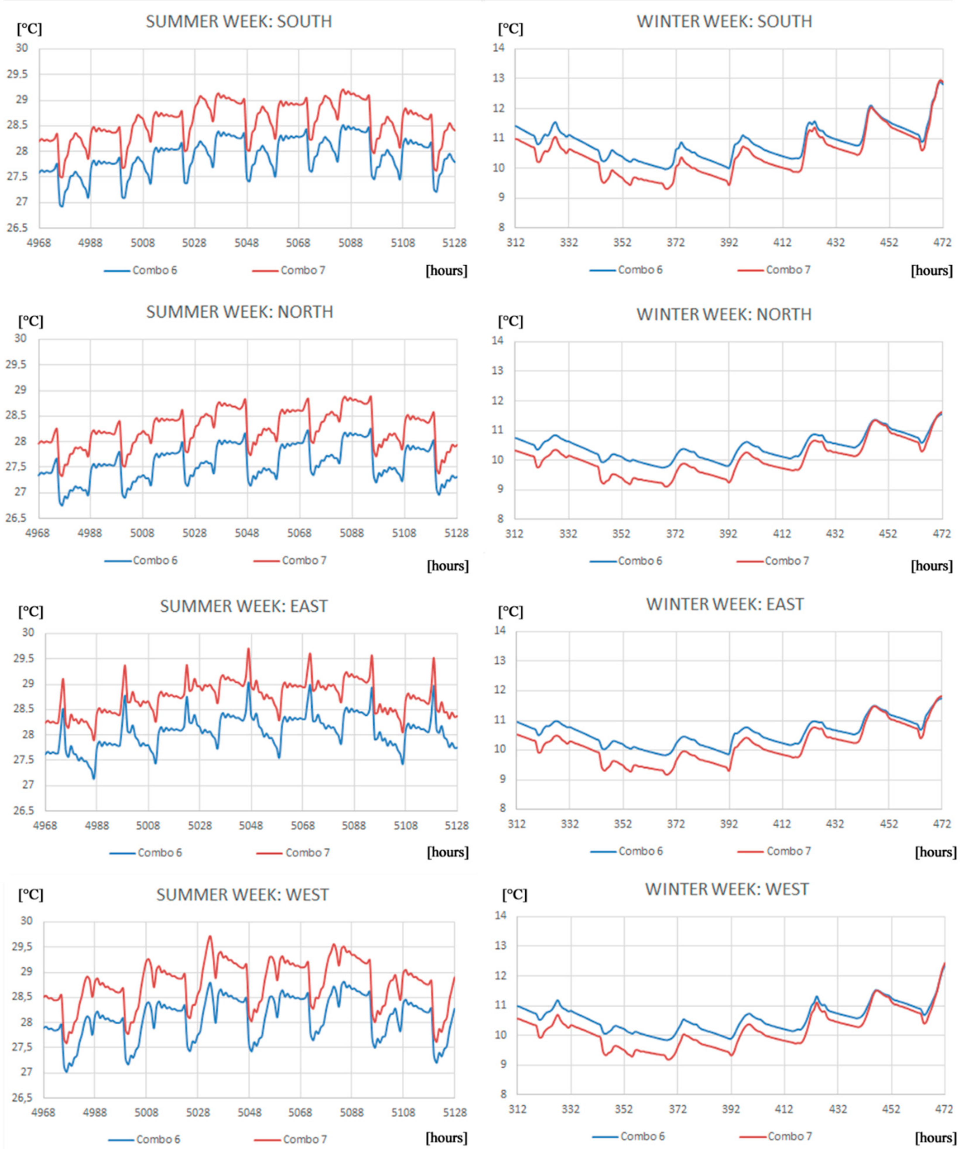
3.4. The Fourth Step: Evaluation of the Number of Pipes
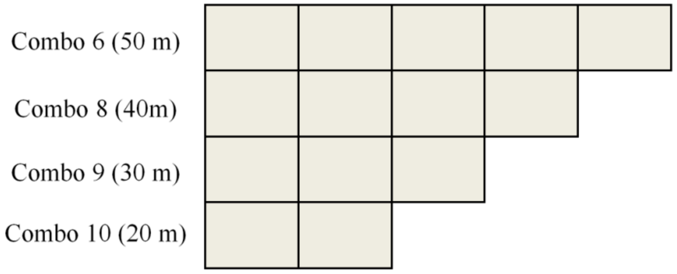
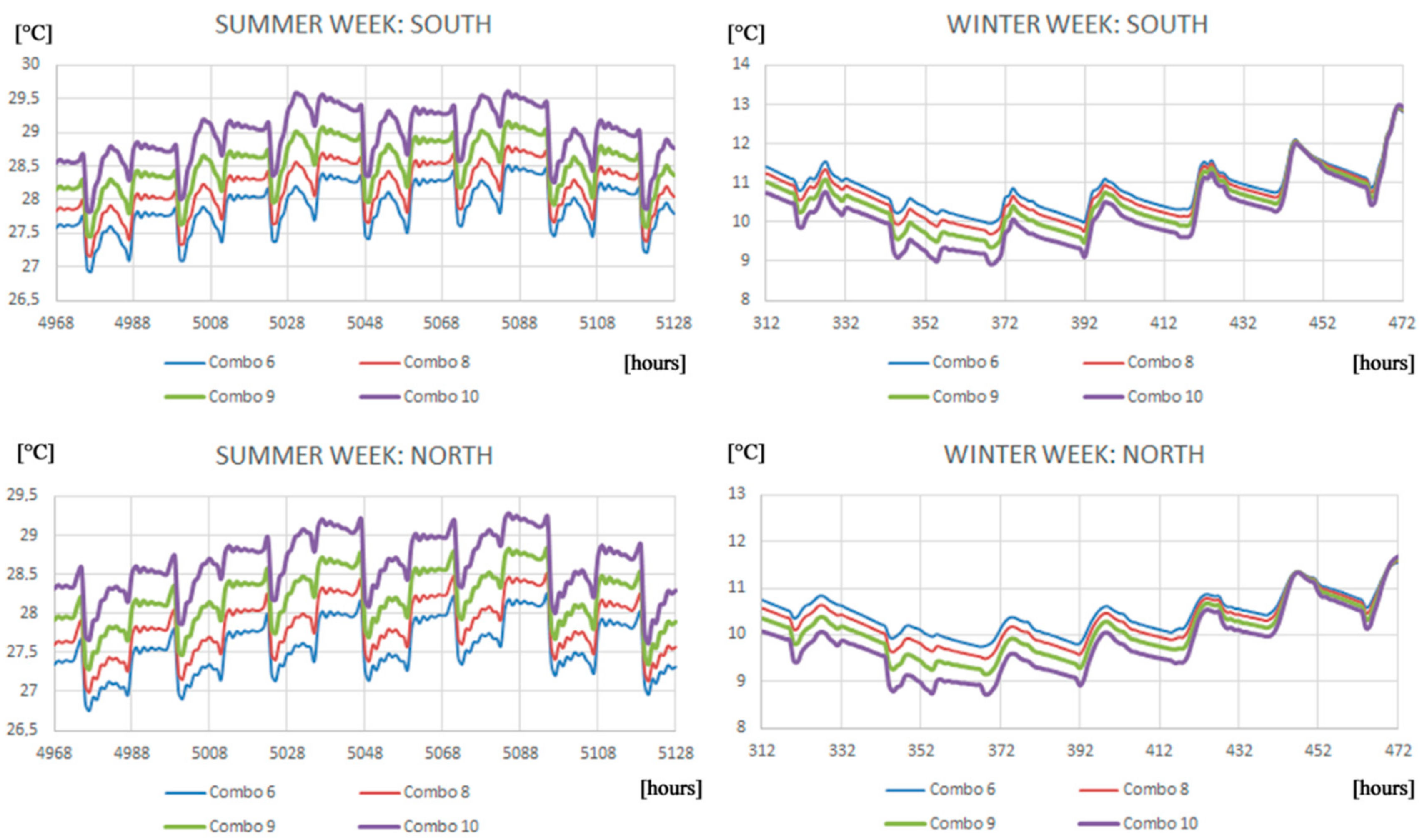
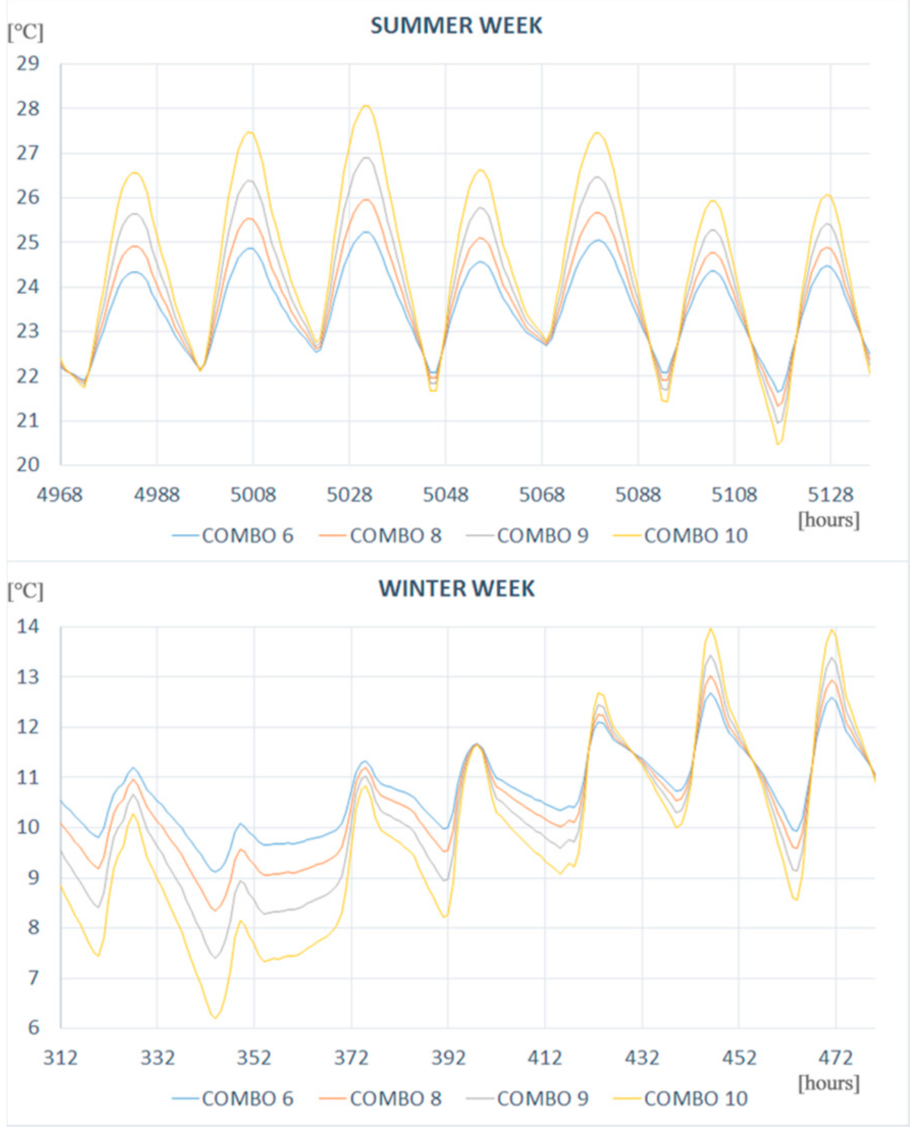
3.5. The Fifth Step: Study of the Length of the Pipe
3.6. The Sixth Step: Different Ground Thermal Conductivity Evaluation (Geothermal System)
4. Conclusions
Author Contributions
Acknowledgments
Conflicts of Interest
Nomenclature
| TOP | Operative air temperature (°C) |
| HVAC | Heating, Ventilation and Air Conditioning |
| HAGHE | Horizontal Air-Ground Heat Exchangers |
| U | Steady thermal transmittance (W/m2K) |
| Ymm | Thermal admittance (W/m2K) |
| Ymn | Periodic thermal transmittance (W/m2K) |
| c | Specific heat capacity (J/kgK) |
| d | Thickness of a layer (m) |
| fd | Decrement factor |
| g | Solar factor |
| t | Time shift: time lead (if positive), or time lag (if negative) (s or h) |
| Ms | Total surface mass (excluding coats) (Kg/m2) |
| fr | Flow rate (m3/h) |
| Subscripts | |
| m, n | For the thermal zones |
| g | Glass |
| f | Frame |
| 1 | Internal |
| 2 | External |
| 22 | From environment to environment |
References
- Taking Stock of the Europe 2020 Strategy for Smart, Sustainable and Inclusive Growth. Available online: https://ec.europa.eu/info/sites/info/files/europe2020stocktaking_annex_en.pdf (accessed on 12 July 2018).
- D’Agostino, D. Assessment of the progress towards the establishment of definitions of Nearly Zero Energy Buildings (NZEBs) in European Member States. J. Build. Eng. 2015, 1, 20–32. [Google Scholar] [CrossRef]
- D’Agostino, D.; Cuniberti, B.; Bertoldi, P. Energy consumption and efficiency technology measures in European non-residential buildings. Energy Build. 2017, 153, 72–86. [Google Scholar] [CrossRef]
- Directive 2010/31/EU on the Energy Performance of Buildings (recast)—19 May 2010. Available online: http://www.buildup.eu/en/practices/publications/directive-201031eu-energy-performance-buildings-recast-19-may-2010 (accessed on 9 August 2018).
- Directive 2012/27/EU of the European Parliament and of the Council of 25 October 2012 on Energy Efficiency. Available online: http://www.buildup.eu/en/practices/publications/directive-201227eu-european-parliament-and-council-25-october-2012-energy (accessed on 9 August 2018).
- Directive 2009/28/EC of the European Parliament and of the Council of 23 April 2009 on the Promotion of the Use of Energy from Renewable Sources and Amending and Subsequently Repealing Directives 2001/77/EC and 2003/30/EC. Available online: http://www.buildup.eu/en/practices/publications/directive-200928ec-european-parliament-and-council-23-april-2009-promotion (accessed on 9 August 2018).
- D’Agostino, D.; Zangheri, P.; Castellazzi, L. Towards Nearly Zero Energy buildings (NZEBs) in Europe: A focus on retrofit in non-residential buildings. Energies 2017, 10, 117. [Google Scholar]
- D’Agostino, D.; Parker, D. A framework for the cost-optimal design of nearly zero energy buildings (NZEBs) in representative climates across Europe. Energy 2018, 149, 814–829. [Google Scholar] [CrossRef]
- D’Agostino, D.; Parker, D. Data on cost-optimal Nearly Zero Energy Buildings (NZEBs) across Europe. Data Brief. 2018, 17, 1168–1174. [Google Scholar] [CrossRef] [PubMed]
- Tian, Z.; Zhang, X.; Jin, X.; Zhou, X.; Si, B.; Shi, X. Towards adoption of building energy simulation and optimization for passive building design: A survey and a review. Energy Build. 2018, 158, 1306–1316. [Google Scholar] [CrossRef]
- Aste, N.; Manfren, M.; Marenzi, G. Building automation and control systems and performance optimization: A framework for analysis. Renew. Sustain. Energy Rev. 2017, 75, 313–330. [Google Scholar] [CrossRef]
- Wright, J.; Loosemore, H.; Farmani, R. Optimization of building thermal design and control by multi-criterion genetic algorithm. Energy Build. 2002, 34, 959–972. [Google Scholar] [CrossRef]
- Bambrook, S.; Sproul, A.; Jacob, D. Design optimisation for a low energy home in Sydney. Energy Build. 2011, 43, 1702–1711. [Google Scholar] [CrossRef]
- Vera, J.; Laukkanen, T.; Sirén, K. Multi-objective optimization of hybrid photovoltaic–thermal collectors integrated in a DHW heating system. Energy Build. 2014, 74, 78–90. [Google Scholar] [CrossRef]
- Stavrakakis, G.; Zervas, P.; Sarimveis, H.; Markatos, N. Optimization of window-openings design for thermal comfort in naturally ventilated buildings. Appl. Math. Model. 2012, 36, 193–211. [Google Scholar] [CrossRef]
- Rapone, G.; Saro, O. Optimisation of curtain wall facades for office buildings by means of PSO algorithm. Energy Build. 2012, 45, 189–196. [Google Scholar] [CrossRef]
- Chantrelle, F.P.; Lahmidi, H.; Keilholz, W.; Mankibi, M.; Michel, P. Development of a multicriteria tool for optimizing the renovation of buildings. Appl. Energy 2011, 88, 1386–1394. [Google Scholar] [CrossRef]
- Huang, S.; Hu, R. Optimum design for indoor humidity by coupling Genetic Algorithm with transient simulation based on Contribution Ratio of Indoor Humidity and Climate analysis. Energy Build. 2012, 47, 208–216. [Google Scholar] [CrossRef]
- Chen, H.; Ooka, R.; Kato, S. Study on optimum design method for pleasant outdoor thermal environment using genetic algorithms (GA) and coupled simulation of convection, radiation and conduction. Build. Environ. 2008, 43, 18–30. [Google Scholar] [CrossRef]
- Eisenhower, B.; O’Neill, Z.; Narayanan, S.; Fonoberov, V.A.; Mezi, I. A methodology for meta model based optimization in building energy models. Energy Build. 2012, 47, 292–301. [Google Scholar] [CrossRef]
- Valdiserri, P.; Biserni, C.; Garai, M. Energy performance of a ventilation system for an apartment according to the Italian regulation. Int. J. Energy Environ. Eng. 2016, 7, 353–359. [Google Scholar] [CrossRef]
- Lucchi, M.; Lorenzini, M.; Valdiserri, P. Energy performance of a ventilation system for a block of apartments with a ground source heat pump as generation system. J. Phys. Conf. Ser. 2017, 796, 1. [Google Scholar] [CrossRef]
- Zhou, L.; Haghighat, F. Optimization of ventilation system design and operation in office environment. Part I: Methodology. Build. Environ. 2009, 44, 651–656. [Google Scholar] [CrossRef]
- Wu, R.; Mavromatidis, G.; Orehounig, K.; Carmeliet, J. Multiobjective optimisation of energy systems and building envelope retrofit in a residential community. Appl. Energy 2017, 190, 634–649. [Google Scholar] [CrossRef]
- Kurnitski, J.; Saari, A.; Kalamees, T.; Vuolle, M.; Niemelä, J.; Tark, T. Cost optimal and nearly zero energy performance requirements for buildings in Estonia. Est. J. Eng. 2013, 19, 183–202. [Google Scholar] [CrossRef]
- Baglivo, C.; Congedo, P.M.; D’Agostino, D.; Zacà, I. Cost-optimal analysis and technical comparison between standard and high efficient mono-residential buildings in a warm climate. Energy 2015, 83, 560–575. [Google Scholar] [CrossRef]
- Zacà, I.; D’Agostino, D.; Congedo, P.M.; Baglivo, C. Assessment of cost-optimality and technical solutions in high performance multi-residential buildings in the Mediterranean area. Energy Build. 2015, 102, 250–265. [Google Scholar] [CrossRef]
- Congedo, P.M.; Baglivo, C.; D’Agostino, D.; Tornese, G.; Zacà, I. Efficient solutions and cost-optimal analysis for existing school buildings. Energies 2016, 9, 851. [Google Scholar] [CrossRef]
- Congedo, P.M.; Baglivo, C.; D’Agostino, D.; Zacà, I. Cost-optimal design for nearly zero energy office buildings located in warm climates. Energy 2015, 91, 967–982. [Google Scholar] [CrossRef]
- Glavič, P.; Lukman, R. Review of sustainability terms and their definitions. J. Clean. Prod. 2007, 15, 1875–1885. [Google Scholar] [CrossRef]
- Zhou, C.; Yin, G.; Hu, X. Multi-objective optimization of material selection for sustainable products: Artificial neural networks and genetic algorithm approach. Mater. Des. 2009, 30, 1209–1215. [Google Scholar] [CrossRef]
- Mora, E.P. Life cycle, sustainability and the transcendent quality of building materials. Build. Environ. 2007, 42, 1329–1334. [Google Scholar] [CrossRef]
- Dammann, S.; Elle, M. Environmental indicators: establishing a common language for green building. Build. Res. Inform. 2006, 34, 387–404. [Google Scholar] [CrossRef]
- Barreca, F. Use of giant reed Arundo Donax L. in rural constructions. Agric. Eng. Int. CIGR J. 2012, 14, 46–52. [Google Scholar]
- Congedo, P.M.; Baglivo, C.; Zacà, I.; D’Agostino, D.; Quarta, F.; Cannoletta, A.; Marti, A.; Ostuni, V. Energy retrofit and environmental sustainability improvement of a historical farmhouse in Southern Italy. Energy Procedia 2017, 133, 367–381. [Google Scholar] [CrossRef]
- Balivo, C.; Congedo, P.M.; Cataldo, M.D.; Coluccia, L.D.; D’Agostino, D. Envelope Design optimization by thermal modelling of a building in a warm climate. Energies 2017, 10, 1808. [Google Scholar] [CrossRef]
- Argiriou, A. Ground cooling. In Passive Cooling of Buildings; Santamouris, M., Asimakopoulos, D., Eds.; Earthscan: New York, NY, USA, 2013; pp. 360–403. [Google Scholar]
- Ascione, F.; Bellia, L.; Minichiello, F. Earth-to-air heat exchangers for Italian climates. Renew. Energy 2011, 36, 2177–2188. [Google Scholar] [CrossRef]
- Pfafferott, J. Evaluation of earth-to-air heat exchangers with a standardised method to calculate energy efficiency. Energy Build. 2003, 35, 971–983. [Google Scholar] [CrossRef]
- Lee, K.H.; Strand, R.K. The cooling and heating potential of an earth tube system in buildings. Energy Build. 2008, 40, 486–494. [Google Scholar] [CrossRef]
- Genchi, Y.; Kikegawa, Y.; Inaba, A. CO2 payback-time assessment of a regional-scale heating and cooling system using a ground source heat-pump in a high energy-consumption area in Tokyo. Appl. Energy 2002, 71, 147–160. [Google Scholar] [CrossRef]
- Dickinson, J.; Jackson, T.; Matthews, M.; Cripps, A. The economic and environmental optimisation of integrating ground source energy systems into buildings. Energy 2009, 34, 2215–2222. [Google Scholar] [CrossRef]
- Esen, H.; Inalli, M.; Esen, M. A techno-economic comparison of ground-coupled and air-coupled heat pump system for space cooling. Build. Environ. 2007, 42, 1955–1965. [Google Scholar] [CrossRef]
- Keil, C.; Plura, S.; Radspieler, M.; Schweigler, C. Application of customized absorption heat pumps for utilization of low-grade heat sources. Appl. Therm. Eng. 2008, 28, 2070–2076. [Google Scholar] [CrossRef]
- Desideri, U.; Sorbi, N.; Arcioni, L.; Leonardi, D. Feasibility study and numerical simulation of a ground source heat pump plant, applied to a residential building. Appl. Therm. Eng. 2011, 31, 3500–3511. [Google Scholar] [CrossRef]
- Li, H.; Yang, H. Study on performance of solar assisted air source heat pump systems for hot water production in Hong Kong. Appl. Energy 2010, 87, 2818–2825. [Google Scholar] [CrossRef]
- Chen, C.; Sun, F.-L.; Feng, L.; Liu, M. Underground water-source loop heat-pump air-conditioning system applied in a residential building in Beijing. Appl. Energy 2005, 82, 331–344. [Google Scholar] [CrossRef]
- Lund, J.W.; Freeston, D.H.; Boyd, T.L. Direct application of geothermal energy: 2005 worldwide review. Geothermics 2005, 34, 691–727. [Google Scholar] [CrossRef]
- Wu, Y.; Gan, G.; Verhoef, A.; Vidale, P.L.; Gonzalez, R.G. Experimental measurement and numerical simulation of horizontal-coupled slinky ground source heat exchangers. Appl. Therm. Eng. 2010, 30, 2574–2583. [Google Scholar] [CrossRef]
- Congedo, P.; Lorusso, C.; De Giorgi, M.; Laforgia, D. Computational fluid dynamic modeling of horizontal Air-Ground Heat Exchangers (HAGHE) for HVAC Systems. Energies 2014, 7, 8465–8482. [Google Scholar] [CrossRef]
- Congedo, P.M.; Lorusso, C.; Giorgi, M.G.D.; Marti, R.; D’Agostino, D. Horizontal air-ground heat exchanger performance and humidity simulation by computational fluid dynamic analysis. Energies 2016, 9, 930. [Google Scholar] [CrossRef]
- Congedo, P.M.; Colangelo, G.; Starace, G. CFD simulations of horizontal ground heat exchangers: A comparison among different configurations. Appl. Therm. Eng. 2012, 33, 24–32. [Google Scholar] [CrossRef]
- D’Agostino, D.; Congedo, P.M. CFD modeling and moisture dynamics implications of ventilation scenarios in historical buildings. Build. Environ. 2014, 79, 181–193. [Google Scholar] [CrossRef]
- Bradley, D.; Kummert, M. New evolutions in TRNSYS—A selection of Version 16 features. In Proceedings of the Ninth International IBPSA Conference, Montréal, QC, Canada, 15–18 August 2005; pp. 107–114. [Google Scholar]


| Pipe Parameters | Nominal Diameter | 0.2 | m |
| Thermal Conductivity of Pipe Material | 0.40 | W/mK | |
| Air Parameters | Density of Air | 1.205 | kg/m3 |
| Thermal Conductivity of Air | 0.026 | W/mK | |
| Specific Heat of Air | 1.005 | kJ/kgK | |
| Viscosity of Air | 1.81 × 10⁻⁵ | kg/ms | |
| Initial Temperature of Air | 10.1 | °C | |
| Ground Parameters | Ground Thermal Conductivity | 1 | W/mK |
| 2 | W/mK | ||
| 3 | W/mK | ||
| Density of Ground | 2723 | kg/m3 | |
| Specific Heat of Ground | 0.837 | kJ/kgK | |
| Average Surface Temperature | 16.7 | °C | |
| Amplitude of Surface Temperature | 18.8 | °C | |
| Time Shift | 45 | day | |
| Finite Elements Calculation Set up | Number of Fluid Nodes | 200 (L = 20 m) | - |
| 250 (L = 25 m) | - | ||
| 300 (L = 30 m) | - | ||
| 400 (L = 40 m) | - | ||
| 500 (L = 50 m) | - | ||
| Number of Radial Ground Nodes | −1 | - | |
| Number of Axial Ground Nodes | 20 | - | |
| Number of Circumferential Ground Nodes | 8 | - | |
| Smallest Node Size | 0.2 | m | |
| Node Size Multiplier | 1.2 | - | |
| Farfield Distance | 1 | m |
| Properties | Material | (W/m·K) | c (J/Kg·K) | Thickness (cm) | |
|---|---|---|---|---|---|
| Wall (Internal to External Side) | Tuff | 1.7 | 850 | 2300 | 10 |
| Brick | 0.13 | 1000 | 600 | 20 | |
| Polystyrene | 0.034 | 1700 | 35 | 8 | |
| Ground Floor | Stoneware flooring | 1.47 | 850 | 1700 | 1.5 |
| Concrete (1200 kg/m3) | 0.47 | 850 | 1200 | 8 | |
| Concrete (1600 kg/m3) | 0.73 | 850 | 1600 | 5 | |
| Igloo | 0.072 | 850 | 1000 | 16 | |
| Screed ordinary concrete | 1.06 | 850 | 1700 | 5 | |
| Gravel | 1.2 | 850 | 1700 | 1 | |
| Ceiling | Hollow-core concrete | 0.743 | 850 | 1800 | 25 |
| Concrete (400 kg/m3) | 0.19 | 850 | 400 | 10 | |
| XPS polystyrene panel | 0.04 | 850 | 35 | 8 | |
| Tuff | 1.7 | 850 | 2300 | 10 | |
| Bricks tuff | 0.55 | 850 | 1600 | 5 |
| Properties | Material | U W/m2K | Y12 W/m2K | Y22 W/m2K | Y11 W/m2K | fd | Ms Kg/m2 | ∆t h | k1 kJ/m2K | k 2 kJ/m2K | dm |
|---|---|---|---|---|---|---|---|---|---|---|---|
| Wall (Internal to External Side) | tuff | 0.243 | 0.019 | 0.423 | 5.841 | 0.078 | 352.8 | 14.53 | 80.43 | 5.93 | 0.38 |
| brick | |||||||||||
| polystyrene | |||||||||||
| Ground Floor (Internal to External Side) | stoneware flooring | 0.349 | 0.016 | 3.62 | 3.982 | 0.047 | 463.5 | 19.44 | 3.982 | 3.62 | 0.365 |
| concrete (1200 kg/m3) | |||||||||||
| concrete (1600 kg/m3) | |||||||||||
| igloo | |||||||||||
| screed ordinary concrete | |||||||||||
| gravel | |||||||||||
| Ceiling (Internal to External Side) | hollow-core concrete | 0.314 | 0.012 | 7.39 | 4.50 | 0.039 | 803 | 17.93 | 61.8 | 101.6 | 0.580 |
| concrete (400 kg/m3) | |||||||||||
| xps polystyrene panel | |||||||||||
| tuff | |||||||||||
| bricks tuff |
| Window Measures | Ug (W/m2K) | g | % Frame | Uf (W/m2K) |
|---|---|---|---|---|
| 6/16/6 argon | 1.3 | 0.333 | 15 | 2.27 |
| Descriptions | Values | Hour | |
|---|---|---|---|
| from | to | ||
| Number of occupants | 4 | 0:00 | 24:00 |
| Internal gains of occupants | 100 W | 0:00 | 24:00 |
| Artificial lighting | 5 W/m2 | 8:00 | 20:00 |
| Electronic equipment | 3 W/m2 | 0:00 | 24:00 |
| First step | Different ground thermal conductivity evaluation (no geothermal system) | Combo 1, 2, 3 |
| Second Step | Analysis of the internal ventilation for different ground thermal conductivities (no geothermal system) | Combo 1v, 2v, 3v |
| Third Step | Analysis of different single pipe flow rates | Combo 2, 2v, 4, 5, 6 |
| Fourth Step | Evaluation of the number of pipes | Combo 6, 7 |
| Fifth Step | Study of the length of the pipe | Combo 6, 8, 9, 10 |
| Sixth Step | Different ground thermal conductivity evaluation (geothermal system) | Combo 11, 12 |
| Combo | Haghe | Number of the Pipes for Room | Total Number of the Pipes | Single Pipe Flow Rate (m3/h) | Total Flow Rate (m3/hr) | Pipe Length (m) | Soil Thermal Conductivity (W/mK) |
|---|---|---|---|---|---|---|---|
| Combo 1 | no | - | - | - | - | - | 1 |
| Combo 2 | no | - | - | - | - | - | 2 |
| Combo 3 | no | - | - | - | - | - | 3 |
| Combo 1v | no | - | - | - | 160 | - | 1 |
| Combo 2v | no | - | - | - | 160 | - | 2 |
| Combo 3v | no | - | - | - | 160 | - | 3 |
| Combo 4 | yes | 2 | 18 | 150 | 2700 | 50 | 2 |
| Combo 5 | yes | 2 | 18 | 187.5 | 3375 | 50 | 2 |
| Combo 6 | yes | 2 | 18 | 225 | 4050 | 50 | 2 |
| Combo 7 | yes | 4 | 36 | 112.5 | 4050 | 25 | 2 |
| Combo 8 | yes | 2 | 18 | 225 | 4050 | 40 | 2 |
| Combo 9 | yes | 2 | 18 | 225 | 4050 | 30 | 2 |
| Combo 10 | yes | 2 | 18 | 225 | 4050 | 20 | 2 |
| Combo 11 | yes | 2 | 18 | 225 | 4050 | 50 | 1 |
| Combo 12 | yes | 2 | 18 | 225 | 4050 | 50 | 3 |
| Winter TOP Peaks (°C) | |||||||||
| Combo | TOP_S | TOP_SE | TOP_W | TOP_E | TOP_N | TOP_SW | TOP_CENTRAL | TOP_NW | TOP_NE |
| Combo 1 | 10.67 | 10.33 | 10.42 | 10.40 | 10.24 | 10.34 | 10.80 | 9.95 | 9.98 |
| 17 January (8:00) | 17 January (8:00) | 17 January (8:00) | 17 January (8:00) | 16 February (7:00) | 17 January (8:00) | 18 January (8:00) | 16 February (7:00) | 17 January (8:00) | |
| Combo 2 | 10.50 | 10.17 | 10.24 | 10.23 | 10.07 | 10.18 | 10.61 | 9.81 | 9.82 |
| 17 January (8:00) | 17 January (8:00) | 17 January (8:00) | 17 January (8:00) | 17 January (8:00) | 17 January (8:00) | 18 January (8:00) | 17 January (8:00) | 17 January (8:00) | |
| Combo 3 | 10.42 | 10.10 | 10.17 | 10.15 | 9.99 | 10.11 | 10.52 | 9.73 | 9.75 |
| 17 January (8:00) | 17 January (8:00) | 17 January (8:00) | 17 January (8:00) | 17 January (8:00) | 17 January (8:00) | 18 January (8:00) | 17 January (8:00) | 17 January (8:00) | |
| Summer TOP Peaks (°C) | |||||||||
| Combo | TOP_S | TOP_SE | TOP_W | TOP_E | TOP_N | TOP_SW | TOP_CENTRAL | TOP_NW | TOP_NE |
| Combo 1 | 34.56 | 34.35 | 35.00 | 34.53 | 33.56 | 34.52 | 34.16 | 33.70 | 33.48 |
| 21 August (14:00) | 21 August (14:00)) | 29 July (17:00) | 30 July (10:00) | 31 July (18:00) | 31 August (16:00) | 31 July (20:00) | 31 July (17:00) | 30 July (10:00) | |
| Combo 2 | 34.69 | 34.47 | 35.16 | 34.69 | 33.72 | 34.61 | 34.34 | 33.85 | 33.63 |
| 21 August (14:00) | 21 August (14:00) | 29 July (17:00) | 30 July (10:00) | 31 July (18:00) | 31 August (16:00) | 31 July (20:00) | 31 July (17:00) | 30 July (10:00) | |
| Combo 3 | 34.75 | 34.52 | 35.23 | 34.76 | 33.80 | 34.66 | 34.42 | 33.92 | 33.70 |
| 21 August (14:00) | 21 August (14:00) | 29 July (17:00) | 30 July (10:00) | 31 July (18:00) | 31 August (16:00) | 31 July (20:00) | 31 July (17:00) | 30 July (10:00) | |
| Winter TOP Peaks (°C) | |||||||||
| Combo | TOP_S | TOP_SE | TOP_W | TOP_E | TOP_N | TOP_SW | TOP_CENTRAL | TOP_NW | TOP_NE |
| Combo 1v | 10.07 | 9.79 | 9.84 | 9.83 | 9.68 | 9.79 | 10.17 | 9.45 | 9.44 |
| 17 January (8:00) | 17 January (8:00) | 17 January (8:00) | 17 January (8:00) | 17 January (8:00) | 17 January (8:00) | 17 January (8:00) | 17 January (8:00) | 17 January (8:00) | |
| Combo 2v | 9.92 | 9.65 | 9.69 | 9.67 | 9.53 | 9.66 | 10.01 | 9.31 | 9.30 |
| 17 January (8:00) | 17 January (8:00) | 17 January (8:00) | 17 January (8:00) | 17 January (8:00) | 17 January (8:00) | 17 January (8:00) | 17 January (8:00) | 17 January (8:00) | |
| Combo 3v | 9.86 | 9.58 | 9.62 | 9.61 | 9.46 | 9.59 | 9.93 | 9.25 | 9.24 |
| 17 January (8:00) | 17 January (8:00) | 17 January (8:00) | 17 January (8:00) | 17 January (8:00) | 17 January (8:00) | 17 January (8:00) | 17 January (8:00) | 17 January (8:00) | |
| Summer TOP Peaks (°C) | |||||||||
| Combo | TOP_S | TOP_SE | TOP_W | TOP_E | TOP_N | TOP_SW | TOP_CENTRAL | TOP_NW | TOP_NE |
| Combo 1v | 33.65 | 33.51 | 34.13 | 33.57 | 32.69 | 33.68 | 33.18 | 32.89 | 32.66 |
| 21 August (14:00) | 21 August (14:00) | 29 July (17:00) | 30 July (10:00) | 31 July (18:00) | 31 August (16:00) | 31 July (20:00) | 31 July (17:00) | 30 July (10:00) | |
| Combo 2v | 33.76 | 33.61 | 34.27 | 33.71 | 32.83 | 33.77 | 33.33 | 33.02 | 32.79 |
| 21 August (14:00) | 21 August (14:00) | 29 July (17:00) | 30 July (10:00) | 31 July (18:00) | 31 August (16:00) | 31 July (20:00) | 31 July (17:00) | 30 July (10:00) | |
| Combo 3v | 33.80 | 33.66 | 34.34 | 33.77 | 32.90 | 33.80 | 33.40 | 33.08 | 32.85 |
| 21 August (14:00) | 21 August (14:00) | 29 July (17:00) | 30 July (10:00) | 31 July (18:00) | 31 August (16:00) | 31 July (20:00) | 31 July (17:00) | 30 July (10:00) | |
| Yearly Hours | Daily Hours | T ext (°C) | UR ext | T out Combo 4 | UR out Combo 4 | T out Combo 6 | UR out Combo 6 | Yearly Hours | Daily Hours | T ext (°C) | UR ext | T out Combo 4 | UR out Combo 4 | T out Combo 6 | UR out Combo 6 |
|---|---|---|---|---|---|---|---|---|---|---|---|---|---|---|---|
| 4976 | 8 | 24.15 | 0.90 | 22.69 | 0.98 | 22.75 | 0.98 | 5072 | 8 | 25.25 | 0.80 | 23.37 | 0.89 | 23.45 | 0.88 |
| 4977 | 9 | 25.1 | 0.80 | 22.97 | 0.89 | 23.05 | 0.89 | 5073 | 9 | 26.35 | 0.60 | 23.68 | 0.67 | 23.79 | 0.67 |
| 4978 | 10 | 26.15 | 0.80 | 23.27 | 0.96 | 23.39 | 0.89 | 5074 | 10 | 27.35 | 0.60 | 23.97 | 0.73 | 24.11 | 0.60 |
| 4979 | 11 | 27.2 | 0.90 | 23.57 | 1.00 | 23.72 | 1.00 | 5075 | 11 | 28.2 | 0.60 | 24.22 | 0.76 | 24.38 | 0.75 |
| 498 | 12 | 28.05 | 0.80 | 23.82 | 1.00 | 23.99 | 1.00 | 5076 | 12 | 28.95 | 0.60 | 24.43 | 0.78 | 24.62 | 0.77 |
| 4981 | 13 | 28.65 | 0.70 | 23.99 | 0.92 | 24.18 | 0.89 | 5077 | 13 | 29.55 | 0.50 | 24.61 | 0.66 | 24.81 | 0.66 |
| 4982 | 14 | 29 | 0.70 | 24.09 | 0.92 | 24.30 | 0.92 | 5078 | 14 | 30 | 0.50 | 24.74 | 0.66 | 24.96 | 0.66 |
| 4983 | 15 | 29.15 | 0.60 | 24.14 | 0.79 | 24.35 | 0.78 | 5079 | 15 | 30.3 | 0.60 | 24.83 | 0.79 | 25.05 | 0.79 |
| 4984 | 16 | 29.15 | 0.70 | 24.15 | 0.92 | 24.35 | 0.92 | 508 | 16 | 30.3 | 0.60 | 24.83 | 0.79 | 25.06 | 0.79 |
| 4985 | 17 | 28.95 | 0.80 | 24.09 | 1.00 | 24.29 | 1.00 | 5081 | 17 | 30.05 | 0.70 | 24.77 | 0.92 | 24.98 | 0.90 |
| 4986 | 18 | 28.45 | 0.80 | 23.96 | 1.00 | 24.14 | 1.00 | 5082 | 18 | 29.6 | 0.70 | 24.64 | 0.92 | 24.85 | 0.92 |
| 4987 | 19 | 27.65 | 1.00 | 23.73 | 1.00 | 23.89 | 1.00 | 5083 | 19 | 28.9 | 0.80 | 24.45 | 1.00 | 24.63 | 1.00 |
| 4988 | 20 | 26.9 | 1.00 | 23.52 | 1.00 | 23.66 | 1.00 | 5084 | 20 | 28.05 | 0.90 | 24.21 | 1.00 | 24.37 | 1.00 |
| 5 | 8 | 24.65 | 0.70 | 22.93 | 0.78 | 23.00 | 0.77 | 5096 | 8 | 22.6 | 0.60 | 22.70 | 0.60 | 22.70 | 0.60 |
| 5001 | 9 | 25.95 | 0.60 | 23.30 | 0.67 | 23.41 | 0.67 | 5097 | 9 | 23.6 | 0.50 | 22.99 | 0.50 | 23.02 | 0.50 |
| 5002 | 10 | 27.15 | 0.60 | 23.64 | 0.74 | 23.79 | 0.73 | 5098 | 10 | 24.65 | 0.50 | 23.29 | 0.50 | 23.35 | 0.50 |
| 5003 | 11 | 28.2 | 0.60 | 23.95 | 0.77 | 24.12 | 0.76 | 5099 | 11 | 25.5 | 0.50 | 23.54 | 0.56 | 23.62 | 0.50 |
| 5004 | 12 | 29.15 | 0.60 | 24.22 | 0.79 | 24.42 | 0.79 | 51 | 12 | 26.3 | 0.50 | 23.77 | 0.56 | 23.87 | 0.56 |
| 5005 | 13 | 29.9 | 0.50 | 24.44 | 0.66 | 24.66 | 0.66 | 5101 | 13 | 27 | 0.50 | 23.97 | 0.56 | 24.10 | 0.56 |
| 5006 | 14 | 30.35 | 0.50 | 24.57 | 0.66 | 24.81 | 0.66 | 5102 | 14 | 27.5 | 0.60 | 24.12 | 0.73 | 24.26 | 0.73 |
| 5007 | 15 | 30.55 | 0.60 | 24.63 | 0.85 | 24.87 | 0.79 | 5103 | 15 | 27.8 | 0.60 | 24.21 | 0.74 | 24.35 | 0.73 |
| 5008 | 16 | 30.5 | 0.70 | 24.62 | 0.99 | 24.86 | 0.97 | 5104 | 16 | 27.8 | 0.60 | 24.21 | 0.74 | 24.36 | 0.73 |
| 5009 | 17 | 30.1 | 0.60 | 24.51 | 0.79 | 24.74 | 0.79 | 5105 | 17 | 27.5 | 0.60 | 24.13 | 0.67 | 24.27 | 0.67 |
| 501 | 18 | 29.4 | 0.70 | 24.32 | 0.92 | 24.53 | 0.92 | 5106 | 18 | 26.95 | 0.80 | 23.98 | 0.95 | 24.10 | 0.95 |
| 5011 | 19 | 28.5 | 0.80 | 24.07 | 1.00 | 24.25 | 1.00 | 5107 | 19 | 26.2 | 0.90 | 23.77 | 1.00 | 23.87 | 1.00 |
| 5012 | 20 | 27.7 | 0.80 | 23.84 | 1.00 | 24.00 | 1.00 | 5108 | 20 | 25.4 | 1.00 | 23.55 | 1.00 | 23.62 | 1.00 |
| 5024 | 8 | 25.4 | 0.70 | 23.23 | 0.78 | 23.32 | 0.78 | 512 | 8 | 21.75 | 0.40 | 22.55 | 0.40 | 22.52 | 0.40 |
| 5025 | 9 | 26.75 | 0.70 | 23.62 | 0.84 | 23.75 | 0.78 | 5121 | 9 | 23.1 | 0.40 | 22.93 | 0.40 | 22.94 | 0.40 |
| 5026 | 10 | 28 | 0.70 | 23.98 | 0.89 | 24.14 | 0.88 | 5122 | 10 | 24.35 | 0.50 | 23.29 | 0.50 | 23.34 | 0.50 |
| 5027 | 11 | 29.1 | 0.80 | 24.29 | 1.00 | 24.49 | 1.00 | 5123 | 11 | 25.5 | 0.50 | 23.62 | 0.51 | 23.70 | 0.56 |
| 5028 | 12 | 30 | 0.80 | 24.55 | 1.00 | 24.78 | 1.00 | 5124 | 12 | 26.5 | 0.50 | 23.91 | 0.56 | 24.02 | 0.56 |
| 5029 | 13 | 30.7 | 0.80 | 24.76 | 1.00 | 25 | 1.00 | 5125 | 13 | 27.25 | 0.40 | 24.13 | 0.44 | 24.26 | 0.44 |
| 503 | 14 | 31.15 | 0.70 | 24.89 | 1.00 | 25.14 | 0.99 | 5126 | 14 | 27.75 | 0.40 | 24.27 | 0.44 | 24.42 | 0.44 |
| 5031 | 15 | 31.4 | 0.60 | 24.96 | 0.87 | 25.23 | 0.84 | 5127 | 15 | 27.95 | 0.40 | 24.34 | 0.44 | 24.48 | 0.44 |
| 5032 | 16 | 31.4 | 0.70 | 24.97 | 1.00 | 25.23 | 0.98 | 5128 | 16 | 27.9 | 0.40 | 24.33 | 0.44 | 24.47 | 0.44 |
| 5033 | 17 | 31.1 | 0.70 | 24.89 | 1.00 | 25.14 | 0.99 | 5129 | 17 | 27.5 | 0.30 | 24.22 | 0.33 | 24.35 | 0.33 |
| 5034 | 18 | 30.45 | 0.80 | 24.71 | 1.00 | 24.94 | 1.00 | 513 | 18 | 26.75 | 0.40 | 24.01 | 0.44 | 24.12 | 0.44 |
| 5035 | 19 | 29.5 | 0.90 | 24.44 | 1.00 | 24.65 | 1.00 | 5131 | 19 | 25.8 | 0.50 | 23.74 | 0.56 | 23.83 | 0.50 |
| 5036 | 20 | 28.6 | 0.90 | 24.19 | 1.00 | 24.37 | 1.00 | 5132 | 20 | 24.9 | 0.60 | 23.49 | 0.60 | 23.55 | 0.60 |
| 5048 | 8 | 23.5 | 0.70 | 22.78 | 0.70 | 22.81 | 0.70 | - | - | - | - | - | - | - | - |
| 5049 | 9 | 24.85 | 0.60 | 23.17 | 0.66 | 23.24 | 0.61 | - | - | - | - | - | - | - | - |
| 505 | 10 | 26 | 0.60 | 23.50 | 0.67 | 23.60 | 0.67 | - | - | - | - | - | - | - | - |
| 5051 | 11 | 26.95 | 0.60 | 23.77 | 0.72 | 23.90 | 0.67 | - | - | - | - | - | - | - | - |
| 5052 | 12 | 27.8 | 0.70 | 24.02 | 0.88 | 24.17 | 0.87 | - | - | - | - | - | - | - | - |
| 5053 | 13 | 28.45 | 0.60 | 24.21 | 0.77 | 24.38 | 0.76 | - | - | - | - | - | - | - | - |
| 5054 | 14 | 28.85 | 0.80 | 24.33 | 1.00 | 24.51 | 1.00 | - | - | - | - | - | - | - | - |
| 5055 | 15 | 29.05 | 0.80 | 24.39 | 1.00 | 24.58 | 1.00 | - | - | - | - | - | - | - | - |
| 5056 | 16 | 29 | 0.70 | 24.38 | 0.92 | 24.57 | 0.91 | - | - | - | - | - | - | - | - |
| 5057 | 17 | 28.65 | 0.60 | 24.28 | 0.78 | 24.46 | 0.77 | - | - | - | - | - | - | - | - |
| 5058 | 18 | 28 | 0.70 | 24.10 | 0.88 | 24.26 | 0.87 | - | - | - | - | - | - | - | - |
| 5059 | 19 | 27.1 | 0.80 | 23.85 | 0.97 | 23.98 | 0.96 | - | - | - | - | - | - | - | - |
| 506 | 20 | 26.35 | 0.90 | 23.64 | 1.00 | 23.75 | 1.00 | - | - | - | - | - | - | - | - |
| Winter TOP peaks (°C) | |||||||||
| Combo | TOP_S | TOP_SE | TOP_W | TOP_E | TOP_N | TOP_SW | TOP_CENTRAL | TOP_NW | TOP_NE |
| Combo 6 | 9.10 | 9.10 | 8.72 | 9.05 | 8.56 | 8.95 | 8.91 | 8.44 | 8.43 |
| 16 February (8:00) | 16 February (8:00) | 16 February (8:00) | 16 February (8:00) | 16 February 16 (8:00) | 16 February (8:00) | 16 February (8:00) | 16 February (8:00) | 15 February (8:00) | |
| Combo 7 | 9.05 | 9.05 | 8.67 | 9.00 | 8.51 | 8.90 | 8.86 | 8.39 | 8.20 |
| 16 February (8:00) | 16 February (8:00) | 16 February (8:00) | 16 February (8:00) | 16 February (8:00) | 16 February (8:00) | 16 February (8:00) | 15 February (8:00) | 14 February (8:00) | |
| Summer TOP peaks (°C) | |||||||||
| Combo | TOP_S | TOP_SE | TOP_W | TOP_E | TOP_N | TOP_SW | TOP_CENTRAL | TOP_NW | TOP_NE |
| Combo 6 | 29.71 | 29.81 | 29.97 | 29.65 | 29.34 | 29.93 | 29.54 | 29.37 | 29.36 |
| 31 August (14:00) | 31 August (14:00) | 31 August (17:00) | September 1 (7:00) | 20 August (7:00) | 31 August (16:00) | 20 August (7:00) | 20 August (7:00) | 20 August (7:00) | |
| Combo 7 | 30.14 | 30.23 | 30.54 | 30.17 | 29.79 | 30.38 | 30.04 | 29.80 | 29.78 |
| 31 August (14:00) | 31 August (14:00) | 18 August (17:00) | 23 July (7:00) | 20 August (7:00) | 31 August (16:00) | 20 August (7:00) | 20 August (7:00) | 20 August (7:00) | |
© 2018 by the authors. Licensee MDPI, Basel, Switzerland. This article is an open access article distributed under the terms and conditions of the Creative Commons Attribution (CC BY) license (http://creativecommons.org/licenses/by/4.0/).
Share and Cite
Baglivo, C.; D’Agostino, D.; Congedo, P.M. Design of a Ventilation System Coupled with a Horizontal Air-Ground Heat Exchanger (HAGHE) for a Residential Building in a Warm Climate. Energies 2018, 11, 2122. https://doi.org/10.3390/en11082122
Baglivo C, D’Agostino D, Congedo PM. Design of a Ventilation System Coupled with a Horizontal Air-Ground Heat Exchanger (HAGHE) for a Residential Building in a Warm Climate. Energies. 2018; 11(8):2122. https://doi.org/10.3390/en11082122
Chicago/Turabian StyleBaglivo, Cristina, Delia D’Agostino, and Paolo Maria Congedo. 2018. "Design of a Ventilation System Coupled with a Horizontal Air-Ground Heat Exchanger (HAGHE) for a Residential Building in a Warm Climate" Energies 11, no. 8: 2122. https://doi.org/10.3390/en11082122
APA StyleBaglivo, C., D’Agostino, D., & Congedo, P. M. (2018). Design of a Ventilation System Coupled with a Horizontal Air-Ground Heat Exchanger (HAGHE) for a Residential Building in a Warm Climate. Energies, 11(8), 2122. https://doi.org/10.3390/en11082122