Online Energy Management and Heterogeneous Task Scheduling for Smart Communities with Residential Cogeneration and Renewable Energy

Abstract

With the development of renewable energy technology and communication technology in recent years, many residents now utilize renewable energy devices in their residences with energy storage systems. We have full confidence in the promising prospects of sharing idle energy with others in a community. However, it is a great challenge to share residents’ energy with others in a community to minimize the total cost of all residents. In this paper, we study the problem of energy management and task scheduling for a community with renewable energy and residential cogeneration, such as residential combined heat and power system (resCHP) to pay the least electricity bill. We take elastic and inelastic load demands into account which are delay intolerant and delay tolerant tasks in the community. The minimum cost problem of a non-cooperative community is extracted into a random non-convex optimization problem with some physical constraints. Our objective is to minimize the time-average cost for each resident in the community, including the cost of the external grid and natural gas. The Lyapunov optimization theory and a primal-dual gradient method are adopted to tackle this problem, which needs no future data and has low computational complexity. Furthermore, we design a cooperative renewable energy sharing algorithm based on State-action-reward-state-action (Sarsa) Algorithm, in the condition that each residence in the community is able to communicate with its neighbors by a central controller. Finally, extensive simulations are presented to validate the proposed algorithms by using practical data.

1. Introduction

With the development of renewable energy technology, many residents utilize renewable energy devices in their residences with energy storage systems. Therefore, we have full confidence in the promising prospects of sharing idle energy with others in a community. As a smart grid develops rapidly, energy management systems have been widely utilized in many fields, e.g., Supervisory Control and Data Acquisition [1]. Particularly, a residential combined heat and power (resCHP) [2] system becomes increasingly popular in a smart grid for its relatively low emissions and high efficiency, which can produce electricity and thermal energy simultaneously. In this way, the system will be more efficient and economical than previous systems that generate these two kinds of energy separately. The long-term system cost can be minimized by using large batteries which are used to store electricity. In addition, renewable energy devices such as solar panel or wind turbine are popular in a smart grid, which becomes one typical feature with increasing environmental concerns. However, large-scale integration of renewable energy will cause the power system to destabilize. In this condition, batteries and elastic loads can be utilized to decrease the fluctuation caused by renewable energy. In addition, it is more friendly for the environment to utilize batteries and elastic loads which can do the power dispatching across time [3].

The energy management and optimal scheduling for a smart grid with resCHP system with hybrid renewable energy sources can reduce carbon dioxide emissions. Li et al. [4] proposed a real-time scheduling policy by applying modified Lyapunov optimization to separate and sequentially determine the joint load scheduling and storage control. Yu et al. [5] proposed a real-time and distributed algorithm by applying the Lyapunov optimization method and an alternating direction method of multipliers to solve a stochastic programming problem with many practical constraints. Liu et al. [6] proposed a parallel distributed optimization algorithm to minimize the cost of microgrids and the utility company by applying game theory. Ou et al. [7] utilized a dynamic switch and time-variant control strategies to design a new voltage controller to convert carbon dioxide into methane and methanol, and then studies control strategies for a hybrid energy microgrid [8], where the controller utilized a radial basis function network-sliding algorithm and a general regression neural network for maximum power point tracking (MPPT) control to control real power fast and steadily. In practice, we should pay more attention to the dynamic operation, MPPT and system stability in faults. Hong et al. [9] proposed an intelligent controller including the radial basis function network and the improved neural network for MPPT control. Bui et al. [10] used an agent communication language to develop a modified contract net protocol for different agents’ communication to optimize the operation of microgrids. Ou et al. [11,12] discusses a distributed generator model and a distributed energy resource for both islanded and grid-connected modes. Zhang et al. [13] introduced a power scheduling approach to solve the problem of renewable energy’s stochastic availability. Ou et al. [14] applied a smart damping controller for the static synchronous compensator to reduce the power fluctuations and damping in a hybrid energy microgrid. Mane et al. [15] proposed an improved Lyapunov controller operated in cascade mode to control a hybrid energy microgrid of fuel and an ultracapacitor. Bahrami et al. [16] modified the traditional demand response programs for multiple energy carriers to transfer into an energy center. Mohammadi et al. [17] proposed a method by applying game theory to increase efficiency of the traditional communication network. With the development of information and communication technology, we have a good two-way communication between smart appliances and control centers, which makes it possible to reduce the cost by scheduling the tasks using some demand response strategies, such as real-time price strategy [18]. Smart appliances can schedule their tasks by using a real-time price strategy to avoid the peak for reducing the total system cost and the capacity of generators [19]. Previous researchers designed some algorithms to help the practical system decide when to store electricity, utilize it, or sell it to the grid according to real-time price. Without an appropriate real-time price strategy, some needless peaks will arise, which are unfavourable to coordinate elastic loads [20]. Other researchers focused on scheduling elastic loads without real-time price.

In the paper, we firstly formulate the minimum cost problem of our system into a non-convex optimization problem with physical constraints, which is difficult to handle. Then, this problem is reformulated via relaxing time coupling constraints into a time-averaged constraint. The Lyapunov optimization theory is adopted to handle the reformulated issue. Furthermore, we design an online algorithm for energy management and task scheduling, which does not depend on the statistic system information and has a low computational complexity. Our system model is shown in Figure 1.

We summarize the contributions of our paper as follows:

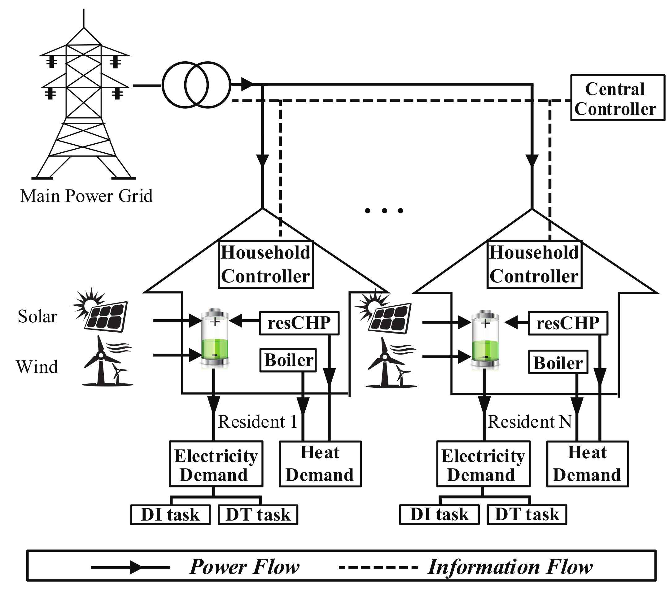
• We propose a practical integrated model that has a resCHP system, a renewable energy device, an energy storage (battery) and a boiler for each residence in the community, extending from other models. Our aim to minimize the time-average cost of the total community, including the cost from the external grid and the gas station. In each residence, we study two cases that is not considered in other models: one has delay intolerant (DI) tasks and the other has delay tolerant (DT) tasks.
• We firstly formulate a cost-optimal problem of one residence in a non-cooperative community in order to reduce the total cost with the constraints of DI and DT tasks. Then, we present an online Task Scheduling Algorithm (TSA) by the Lyapunov optimization approach, which needs no future data and has low computational complexity. Because it is difficult to separate variables, we use a standard primal-dual gradient method to figure out a solution of the problem. For less cost, we propose an energy sharing policy for cooperative energy sharing in the community. By using this policy, we design a cooperative renewable energy sharing algorithm based on a Sarsa algorithm, on the condition that each residence in the community needs to communicate with its neighbors by a central controller.
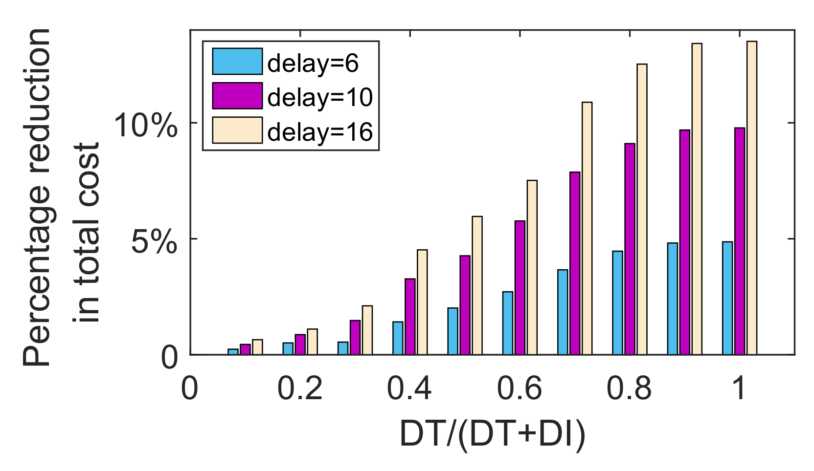
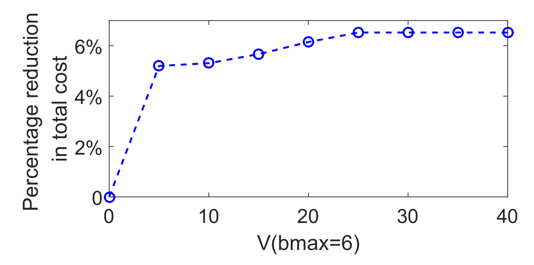
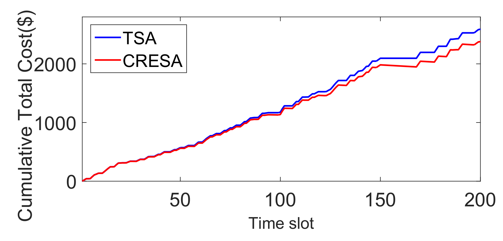
• Extensive simulations are presented to validate the proposed algorithms by using real trace data. The TSA algorithm shows that a larger battery maximum output and V will lead to a higher shaved cost. We satisfy the DT load demand before user-defined deadlines and we can see that, with the increase of the deadline, the saved cost will increase. Compared with the TSA Algorithm (non-cooperative algorithm), the cooperative renewable energy sharing algorithm can reduce a nearly 9% cost for the community while meeting all the demands of the residents.

The rest of this paper consists of the following five sections: Section 2 puts up some questions of an existing resCHP system and task scheduling in a smart grid. Section 3 proposes a system model of a community including resCHP systems, renewable energy devices, energy storage and boilers. We introduce the renewable energy sharing policy and the control target. Section 4 formulates the optimization problem with some constraints in a non-cooperative and cooperative community and gives the details of our designed algorithm. In Section 5, we evaluate the performance of our algorithm by using the real data. Finally, some conclusions are drawn in Section 6.

2. Related Work

With the development of information and communication technology, the traditional power grid has a good chance of upgrading by disposing different kinds of energy sources optimally. The resCHP system becomes increasingly popular in smart grids for its low emissions and high efficiency. Alipour et al. [21] proposed a stochastic programming framework for optimally scheduling, considering uncertainties of demand response. Motevasel et al. [22] proposed an energy management system for optimal scheduling of a microgrid with resCHP to find the optimum point of distributed energy resources, batteries and thermal storage devices. Tasdighi et al. [23] transformed the energy management issue into a mixed-integer linear programming problem for the system using resCHP. Ma et al. [24] designed an energy management framework for resCHP consumers with the demand response using internal prices. In these papers, it is assumed that the electricity price and the load demand in the future is predictable. These studies solve different problems by using Dynamic Programming and the ‘curse of dimensionality’ problem [25] appears.

Many previous studies focused on a designing task scheduling policy. Goudarzi et al. [26] proposed a task scheduling policy that could minimize consumers’ electricity cost by using an inconvenience function. Buttazzo et al. [27] discussed limited preemption models between two cases of fully preemptive and nonpreemptive scheduling. Du et al. [28] proposed a novel linear sequential optimization enhanced multiloop algorithm to schedule load demand considering the satisfaction of consumers. These works tried to design optimal task scheduling algorithms by only considering the convenience of consumers.

There are many optimization methods for reducing the system cost with energy storage in a smart grid. Zhou et al. [29] designed an algorithm about the queueing models of a battery and a tank in the resCHP system to reduce the average cost by adopting a Lyapunov optimization approach. This approach is also used in other papers to optimize the system cost. Neely et al. [30] reduced the average cost of flexible consumers and met deadlines of delay tolerant tasks. Guo et al. [31] considered both DI and DT tasks from the perspective of a household when tackling the problem of minimizing the average cost. Urgaonkar et al. [32] developed an online control algorithm of data center electricity management for minimizing the long-term average cost. However, their models did not include renewables. Liu et al. [33] designed a centralized algorithm to solve the optimization of energy management problem based on adaptive dynamic programming. Gatsis et al. [34] proposed a near-optimal scheduling algorithm considering the Advanced Metering Infrastructure messages between the consumers and the utility company. Logenthiran et al. [35] tackled the problem formulated from day-ahead load shifting method for demand-side management of smart grid by a heuristic-based Evolutionary Algorithm. Koutitas et al. [36] developed a period management strategy of the periodic loads for reducing the cost in a period of time. Their model did not consider task scheduling in the resCHP system. In this paper, we consider the optimal scheduling of DT tasks in a comprehensive system that has a resCHP system, a renewable energy device (e.g., solar panel, wind turbine), a battery and a boiler for each residence to reduce the total cost.

3. System Model and Problem Statement

The overview of our system is shown in Figure 1. There are a set of smart appliances denoted by $i\in \{1,2,\cdots ,N_t\}$ in the residence j and two types of flows, i.e., information and energy flow. For simplicity, we assume that one appliance is utilized in a residence each time slot. We assume that our system works in discrete time slot $t\in \{1,2,\cdots ,T\}$ and T will be 72 h if we study this problem in three days. The details of our system are described as follows.

3.1. System Architecture

This system includes a set of battery, renewable energy devices, boilers and resCHP systems. Let $e_j\left(t\right)$ and $h_j\left(t\right)$ represent the stochastic electricity and heat demand of residence j at time t, respectively. Electricity demand $e_j\left(t\right)$ can be balanced by battery $b_j\left(t\right)$ or external grid $p_j\left(t\right)$. Heat demand $h_j\left(t\right)$ is satisfied by a boiler or the resCHP system for bathing.

In time slot t, the resCHP system of residence j exports electricity ${\eta }_e{u}_j\left(t\right)$ to the battery and ${\eta }_h{u}_j\left(t\right)$ to satisfy heat demand simultaneously, where ${\eta }_e$ and ${\eta }_h$ are the efficiency of converting natural gas to electricity and heat. The resCHP system consumes natural gas $u_j\left(t\right)$. In addition, the battery gets energy $r_j\left(t\right)$ from renewable energy and the boiler exports energy $g_j\left(t\right)$ to satisfy heat demand. We set the electricity price $C_e\left(t\right)$ in the range ($C_{e,min}$, $C_{e,max}$). We assume that the price of natural gas $C_g$ is a constant in each time slot because it does not change greatly. The electricity price $C_e\left(t\right)$ can be obtained from PG & E [37] and the price of natural gas $C_g$ can be known from the report of RateFinder for June 2017 [38] from PG & E. To minimize the average long-term cost, our algorithm focuses on the electricity $p_j\left(t\right)$ bought from the grid and natural gas $u_j\left(t\right)$ consumed by the resCHP and $g_j\left(t\right)$ consumed by the boiler. The symbols used are summarized in Abbreviations.

3.2. Renewables Generation

We assume that there are N residents in a community and all residences are provided with solar panels and wind turbines. From [39], we define that the energy generated from a solar panel $r^s\left(t\right)$ for residence j can be calculated as $r_j^s\left(t\right)=\zeta ·A^j·I\left(t\right)·t^d,r^s\left(t\right)\le r^{s,max}$, where $\zeta$ represents the efficiency of solar energy to electricity, $A^j$ is solar panel area of residence j, $I\left(t\right)$ is the illumination intensity and $t^d$ is the duration of the time slot t. There is an upper bound $r^{s,max}$ for solar energy with the illumination intensity. Also from [39], we define that the energy generated from a wind turbine $r_j^w\left(t\right)$ can be calculated as $r_j^w\left(t\right)=\varsigma ·W{B}_j·\rho v^3\left(t\right)·t_d/2,r_w^j\left(t\right)\le r^{w,max}$, where $\varsigma$ represents the efficiency of wind energy to electricity, $W{B}_j$ is rotor blade area of wind turbine, $\rho$ stands for the density of the air, $v\left(t\right)$ is wind speed and $t^d$ is the duration of time slot t. Obviously, there is an upper bound $r^{w,max}$ for wind energy. In time slot t, the energy converting from renewable energy generators into battery in time slot t for residence j is $r_j\left(t\right)$. We have $r_j\left(t\right)=r_j^s\left(t\right)+r_j^w\left(t\right),r_j\left(t\right)\le r^{s,max}+r^{w,max}$.

3.3. Electricity and Heat Demand

The electricity demand is set as $e_j\left(t\right)$ and the heat demand $h_j\left(t\right)$ for residence j. We assume that tasks are continuous and the electricity consumption rate ${\pi }_j^t$ of each task is constant. Electricity demand is satisfied by the electricity from external grid $p_j\left(t\right)$ and the electricity from battery $b_j\left(t\right)$ in time slot t. Heat demand is satisfied by the resCHP system ${\eta }_h{u}_j\left(t\right)$ and the boiler $g_j\left(t\right)$. According to the energy conservation law, we have the following equation:

$$\begin{array}{cc}\hfill e_j\left(t\right)& =p_j\left(t\right)+b_j\left(t\right),\hfill \end{array}$$

(1)

$$\begin{array}{cc}\hfill h_j\left(t\right)& ={\eta }_h{u}_j\left(t\right)+{\eta }_s{g}_j\left(t\right).\hfill \end{array}$$

(2)

3.4. Delay-Tolerant and Delay-Intolerant Tasks

In this part, we provide a brief introduction to DI and DT tasks. There are some DI tasks in our daily life, such as television or lighting, which needs to be satisfied immediately. DT tasks appear with the advent of smart appliances. With the development of smart appliances, people can make an appointment to do some tasks such as washing and bathing.

In our model, residence use $n_t$ to present the number of tasks $N_t$ that arrive at time slot t. According to the degree of delay tolerance, tasks can be divided into two groups: DT tasks and DI tasks. Each task i∈$N_t$ can be characterized by two parameters: the time needed for the task $a_i^t$ and the deadline for the task $d_i^t$. The task should be finished before $t+d_i^t$. If $a_i^t=d_i^t$, the task should be satisfied immediately; therefore, the task is delay-intolerant. Otherwise, the task is delay-tolerant. For the DI tasks, we cannot propose an ideal scheduling algorithm. We focus on discussing the optimal scheduling algorithm of DT tasks to achieve the minimum cost. The postponing time is set as $s_i^t$ and if the task is delay-tolerant, the postponing time $s_i^t$ is 0. We set $d_{max}\triangleq {max}_{t,i}{d}_i^t$ for the maximum delay of tasks.

3.5. Energy Storage

Here, we do not consider the electricity loss of the battery in the process of charging and discharging. For simplicity, we view the state of the battery as an electricity queue. From Figure 1, we can see that the energy in energy storage in time slot t for the residence i $B_j\left(t\right)$ includes three parts, first from the external grid, second from the renewable energy and the last part from the resCHP system. Thus, the battery level $B_j\left(t\right)$ in time slot t is given in the following equation:

$$B_j(t+1)=B_j\left(t\right)+r_j\left(t\right)+{\eta }_e{u}_j\left(t\right)-b_j\left(t\right).$$

(3)

In general, $p_j\left(t\right)$ has a positive value, and then we see $b_j\left(t\right)$ ≤ $e_j\left(t\right)$ from the aspect of practical application and the constraints are given as follows:

$$\begin{array}{c}|b_j\left(t\right)|\le b_j^{max},\hfill \end{array}$$

(4)

$$\begin{array}{c}{b}_j\left(t\right)\le min\{B_j\left(t\right),e_j\left(t\right)\},\hfill \end{array}$$

(5)

where $b_j^{max}$ is the battery capacity of residence j. The constraint Equations (4) and (5) means that the electricity discharged or charged from the battery has an upper bound in a practical model.

3.6. Energy Sharing Policy

The electricity demand $e_j\left(t\right)$ can be satisfied for residence j as the following expression: $p_j\left(t\right)=e_j\left(t\right)-b_j\left(t\right)+{\sum }_{j\ne i}{r}_{j{j}^{\prime }}\left(t\right)$ residence j can draw or share energy $r_{j{j}^{\prime }}\left(t\right)$ from its neighbor $j^{\prime }$. According to the law of energy conservation, we can obtain that ${\sum }_i{\sum }_{j\ne i}{r}_{j{j}^{\prime }}\left(t\right)=0$.

3.7. Control Target

In time slot t, our system cost consists of the cost from the external grid and natural gas utilized by the resCHP system and the boiler. Electricity demand $e_j\left(t\right)$ is dependent on the task scheduling from time slot t to $t-d_{max}+1$, and we have

$$e_j\left(t\right)={\sum }_{\tau =t-d_{max}+1}^t{\sum }_{i=1}^{n_{\tau }}\psi (\tau +s_j^{\tau }+c_j^{\tau }>t\&\tau +s_j^{\tau }\le t),$$

(6)

and the function $\psi (\tau +s_j^{\tau }+c_j^{\tau }>t\&\tau +s_j^{\tau }\le t)$ is not a specific function. We aim to design a scheduling algorithm to achieve the minimum long-term average cost by assigning the amount of electricity and gas. The long-term average cost can be described as the following expression:

$$C_{tol}^{avg}={lim}_{T\to \infty }\frac{1}{T}{\sum }_{t=1}^T\mathbb{E}\{{\sum }_{i=1}^N{p}_j\left(t\right)C_e\left(t\right)+u_j\left(t\right)C_g+{\eta }_s{g}_j\left(t\right)C_g\}.$$

(7)

For simplicity, we do not consider some practical factors, such as the electricity loss in the transmission in order to focus on minimizing the electricity from a grid related with variables ($s_i^t$, $r\left(t\right)$, $b\left(t\right)$, $u\left(t\right)$, $h\left(t\right)$). We can add these factors into our model in the future.

4. Problem Formulation

In this section, we firstly consider a non-cooperative scenario that residents do not share energy with others. Electricity and heat demand $e\left(t\right)$ and $h\left(t\right)$ are supposed to be independent from each other. According to the system model shown in Figure 1, we firstly assume a convex function of consumers’ dissatisfaction $F_i^t\left(s\right)$ according to [40], which is a utility function of the task i when it delays s time slots. If the delay $s=0$, the value of the function should be zero. As the delay s increases, the utility function will increase, which means that dissatisfaction of consumers increases. The utility function can prove to have a long-term bound $\alpha$ by using the same method in [41]:

$$\underset{T\to \infty }{lim}sup\frac{1}{T}{\sum }_{t=1}^T{\sum }_{i=1}^{n_t}{F}_i^t\left(s_i^t\right)\le \alpha ,$$

(8)

where $s_i^t$ is the delay for the task i. Generally, we should fulfill a task before its deadline, and the constraint for $s_i^t$ is given as the following expression:

$$0\le s_i^t\le d_i^t-a_i^t.$$

(9)

The optimization problem can be summarized as follows:

$$\begin{array}{cc}\hfill \underset{\begin{array}{c}{r}_j\left(t\right),s_i^t,\\ b_j\left(t\right),u_j\left(t\right)\end{array}}{min}& \underset{T\to \infty }{lim}\frac{1}{T}\sum _{t=1}^{T}E[p_j\left(t\right)C_e\left(t\right)+(u_j\left(t\right)+{\eta }_s{g}_j\left(t\right))C_g],\hfill \end{array}$$

(10)

$$\mathrm{s}.\mathrm{t}.\left(1\right),\left(2\right),\left(3\right),\left(4\right),\left(5\right),\left(6\right),\left(8\right),\left(9\right),$$

where $C_e\left(t\right)p\left(t\right)+u\left(t\right)C_g+{\eta }_{s}g\left(t\right)C_g$ is the total cost of the system in time slot t.

According to the equation Equations (1) and (2), we can simplify this problem as P1:

$$\begin{array}{cc}\hfill \mathrm{P}1:\underset{\begin{array}{c}{r}_j\left(t\right),s_i^t,\\ b_j\left(t\right),u_j\left(t\right)\end{array}}{min}& \underset{T\to \infty }{lim}\frac{1}{T}\sum _{t=1}^{T}E[(e_j\left(t\right)-b_j\left(t\right))C_e\left(t\right)+u_j\left(t\right)C_g\hfill \\ & +(h_j\left(t\right)-{\eta }_h{u}_j\left(t\right))C_g],\hfill \end{array}$$

(11)

$$\mathrm{s}.\mathrm{t}.\left(3\right),\left(4\right),\left(5\right),\left(6\right),\left(8\right),\left(9\right).$$

We know that ${lim}_{T\to \infty }{\sum }_{t=1}^T$ $e_j\left(t\right)C_e\left(t\right)$ is the total cost of power demand. We have the following equation:

$$\underset{T\to \infty }{lim}{\sum }_{t=1}^T{e}_j\left(t\right)C_e\left(t\right)=\underset{T\to \infty }{lim}{\sum }_{t=1}^T{\sum }_{i=1}^{n_t}{\sum }_{j=0}^{a_i^t-1}{\pi }_i^t{C}_e(j+t+s_i^t),$$

(12)

where ${\pi }_i^t$ is the electricity consumption rate. We rewrite the optimization problem as the following P2:

$$\begin{array}{cc}\hfill \mathrm{P}2:\underset{\begin{array}{c}{r}_j\left(t\right),s_i^t,\\ b_j\left(t\right),u_j\left(t\right)\end{array}}{min}& \underset{T\to \infty }{lim}\frac{1}{T}\sum _{t=1}^{T}E[\sum _{i=1}^{n_t}\sum _{j=0}^{a_i^t-1}{\pi }_i^t{C}_e(j+t+s_i^t)\hfill \\ & -b_j\left(t\right)C_e\left(t\right)+{\eta }_e{u}_j\left(t\right)C_g+h_j\left(t\right)C_g],\hfill \end{array}$$

(13)

$$\mathrm{s}.\mathrm{t}.\left(3\right),\left(4\right),\left(5\right),\left(6\right),\left(8\right),\left(9\right),$$

P2 is the simplified problem of P1. To solve P2, we use the Lyapunov optimization method [42].

To ensure that dissatisfaction of consumers has a upper bound, we create a virtual queue $J\left(t\right)$ as the following:

$$J(t+1)=max\{J\left(t\right)+{\sum }_{i=1}^{n_t}{F}_i^t\left(s_i^t\right)-\alpha ,0\}.$$

(14)

We can prove that if this virtual queue $J\left(t\right)$ meets the restriction $lim{sup}_{T\to \infty }J\left(T\right)/T=0$ , then we have

$$\underset{T\to \infty }{lim}sup\frac{1}{T}{\sum }_{t=1}^T{\sum }_{i=1}^{n_t}{F}_i^t\left(s_i^t\right)\le \alpha .$$

(15)

4.1. The Lower Bound of the Minimum Cost

In this part, we prove that the minimum cost of P2 has a lower bound. We set C and $\tilde{C}$ to be the minimum cost of P2 and P3:

$$\begin{array}{c}\mathrm{P}3:\underset{\begin{array}{c}{r}_j\left(t\right),s_i^t,\\ b_j\left(t\right),u_j\left(t\right)\end{array}}{min}\underset{T\to \infty }{lim}\frac{1}{T}\sum _{t=1}^{T}E[\sum _{i=1}^{n_t}\sum _{j=0}^{a_i^t-1}{\pi }_i^t{C}_e(j+t+s_i^t)-b\left(t\right)C_e\left(t\right)+{\eta }_e{u}_j\left(t\right)C_g+h_j\left(t\right)C_g],\hfill \\ \mathrm{s}.\mathrm{t}.\left(3\right),\left(5\right),\left(8\right),\left(9\right).\hfill \end{array}$$

We can see that P3 is a relaxation of P2 and $\tilde{C}$ is the lower bound of C. We use Theorem $4.5$ in [43] to prove that $\tilde{C}$ can be calculated according to an optimal randomized stationary policy $\tilde{b}\left(t\right)$.

Lemma 1.

We can get $\tilde{C}$ from an optimal randomized stationary policy that only depends on the system state. The control variables ($\tilde{r}\left(t\right),{\tilde{s}}_i^t,\tilde{b}\left(t\right),\tilde{u}\left(t\right)$) are some functions of [$n_t,c_{tj},r\left(t\right),e\left(t\right),h\left(t\right)$] in each time slot. We have these functions as follows:

$$\begin{array}{c}E[\sum _{i=1}^{n_t}\sum _{j=0}^{a_i^t-1}{\pi }_i^{t}P(j+t+{\tilde{s}}_i^t)-\tilde{b}\left(t\right)C_e\left(t\right)\hfill \\ +{\eta }_e\tilde{u}\left(t\right)C_g+h\left(t\right)C_g]=\tilde{C},\hfill \end{array}$$

(16)

$$\begin{array}{c}E[\sum _{i=1}^{n_t}{F}_i^t\left({\tilde{s}}_i^t\right)-\alpha ]\le 0,\hfill \end{array}$$

(17)

$$\begin{array}{c}E[\tilde{r}\left(t\right)-\tilde{b}\left(t\right)]\ge 0.\hfill \end{array}$$

(18)

Proof. 

We prove it by using Theorem $4.5$ in [43]. Our problem satisfies all sufficient conditions proposed in Theorem $4.5$ for the existence of an optimal randomized stationary policy. Equation (18) means that the long-term average dissatisfaction is no less than $\alpha$. Equations (18) and (19) shows that $B_j\left(t\right)$ and $J\left(t\right)$ have a long-term average stability. Finally, $\tilde{C}$ can be calculated by an optimal randomized stationary policy ($\tilde{r}\left(t\right),{\tilde{s}}_i^t,\tilde{b}\left(t\right),\tilde{u}\left(t\right),\tilde{h}\left(t\right)$). ☐

4.2. TSA: Task Scheduling Algorithm

We usually use Lyapunov drift to study optimal control of queueing networks. By the Lyapunov drift, we can stabilize these two queues $B_j\left(t\right)$ and $J_j\left(t\right)$ for each residence j. We add a weighted penalty term V to the drift of a Lyapunov function $L_j\left(t\right)$. Based on this method, we design a function $L_j\left(t\right)=\frac{1}{2}(J_j{\left(t\right)}^2+{(B_j\left(t\right)-\epsilon )}^2)$. One part of our goal is to minimize the drift of $L_j\left(t\right)$, making $B_j\left(t\right)$ closer to the constant $\epsilon$ where the battery level $B_j\left(t\right)$ is bounded. We have several constants $n_{max}={max}_t{n}_t$, $r_j^{max}={max}_t{r}_j\left(t\right)$, $a_{max}={max}_{t,i}{a}_t^i$, $F_{max}={max}_{t,i}{F}_t^i\left(d_t^i\right)$. We set $Z_j\left(t\right)=(J_j\left(t\right),B_j\left(t\right))$. From the Lyapunov approach, we define the drift is $\Delta =E\left\{(L_j(t+1)-L_j\left(t\right))\right|Z_j\left(t\right)\}$.

Lemma 2.

The Lyapunov drift will satisfy

$$\begin{array}{cc}\hfill \Delta & \le J_j\left(t\right)E[\sum _{i=1}^{n_t}{F}_i^t\left(s_i^t\right)-\alpha |Z_j\left(t\right)]+\frac{1}{2}{[r_j\left(t\right)+{\eta }_e{u}_j\left(t\right)-b_j\left(t\right)]}^2\hfill \\ & +(B_j\left(t\right)-\epsilon )(r_j\left(t\right)+{\eta }_e{u}_j\left(t\right)-b_j\left(t\right))+D,\hfill \end{array}$$

(19)

where D $\triangleq \frac{1}{2}(n_{max}^2{F}_{max}^2+{\alpha }^2)$. The Lyapunov drift Δ can be calculated from $J_j\left(t\right)$ and $B_j\left(t\right)$. We make some simplification to minimize the Lyapunov drift Δ.

Proof. 

We first square Equation (14) of $J\left(t\right)$. By using $max{[x,0]}^2\le x^2$, we have

$$\begin{array}{c}\frac{1}{2}J{(t+1)}^2-\frac{1}{2}J{\left(t\right)}^2\hfill \\ \le \frac{1}{2}{(\sum _{i=1}{n}_t{F}_i^t\left(s_i^t\right)-\alpha )}^2+J\left(t\right)(\sum _{i=1}^{n_t}{F}_i^t\left(s_i^t\right)-\alpha )\hfill \\ \le \frac{1}{2}{n}_{max}^2{F}_{max}^2+\frac{1}{2}{\alpha }^2+J\left(t\right)\sum _{i=1}^{n_t}{F}_i^t\left(s_i^t\right).\hfill \end{array}$$

Then, we square Equation (3) of $B_j\left(t\right)$. By using some parameters that we defined in the previous expression, we have

$$\begin{array}{c}\frac{1}{2}{[B_j(t+1)-\epsilon )}^2-{(B_j\left(t\right)-\epsilon )}^2]\hfill \\ =\frac{1}{2}[B_j{(t+1)}^2-B_j{\left(t\right)}^2]-\epsilon [B_j(t+1)-B_j\left(t\right)]\hfill \\ \le [B_j\left(t\right)-\epsilon ][(r\left(t\right)+{\eta }_{e}u\left(t\right)-b\left(t\right)]+\frac{1}{2}{[r\left(t\right)+{\eta }_{e}u\left(t\right)-b\left(t\right)]}^2.\hfill \end{array}$$

Finally, we figure out the Lyapunov drift $L(t+1)-L\left(t\right)$ as follows:

$$\begin{array}{c}L(t+1)-L\left(t\right)\hfill \\ =\frac{1}{2}[J{(t+1)}^2+{(B_j(t+1)-\epsilon )}^2]-\frac{1}{2}{(J{\left(t\right)}^2+B_j\left(t\right)-\epsilon )}^2)\hfill \\ =\frac{1}{2}J{(t+1)}^2-\frac{1}{2}J{\left(t\right)}^2+\frac{1}{2}{[B_j(t+1)-\epsilon ]}^2-\frac{1}{2}{[B_j\left(t\right)-\epsilon ]}^2\hfill \\ \le \frac{1}{2}{n}_{max}^2{F}_{max}^2+\frac{1}{2}{\alpha }^2+J\left(t\right)\sum _{i=1}^{n_t}{F}_i^t\left(s_i^t\right)+[B_j\left(t\right)-\epsilon ][r\left(t\right)\hfill \\ +{\eta }_{e}u\left(t\right)-b\left(t\right)]+\frac{1}{2}{[r\left(t\right)+{\eta }_{e}u\left(t\right)-b\left(t\right)]}^2.\hfill \end{array}$$

☐

According to the stochastic optimization technique, the Lyapunov drift $\Delta$ should be minimized to make the queue of consumers’ satisfaction $J_j\left(t\right)$ and the queue of battery level $B_j\left(t\right)$ mean rate stable. We also aim to minimize the system cost, so we set a parameter V denoting the trade-off between the system cost and the Lyapunov drift $\Delta$; then, we add $VE[{\sum }_{i=1}^{n_t}{\sum }_{j=0}^{a_i^t-1}{\pi }_i^t{C}_e(j+t+s_i^t)-b_j\left(t\right)C_e\left(t\right)+{\eta }_e{u}_j\left(t\right)C_g+h_j\left(t\right)C_g]$ on both sides of Equation (19), we have

$$\begin{array}{c}\Delta +VE[\sum _{i=1}^{n_t}\sum _{j=0}^{a_i^t-1}{\pi }_i^t{C}_e(j+t+s_i^t)-b_j\left(t\right)C_e\left(t\right)\hfill \\ +{\eta }_e{u}_j\left(t\right)C_g+h_j\left(t\right)C_g]\hfill \\ \le \sum _{i=1}^{n_t}E[J_j\left(t\right)F_i^t\left(s_i^t\right)+V\sum _{j=0}^{a_i^t-1}{\pi }_i^{t}P(j+s_i^t+t)|Z_j\left(t\right)\hfill \\ +D-\alpha J_j\left(t\right)+E[(B_j\left(t\right)-\epsilon )(r_j\left(t\right)+{\eta }_e{u}_j\left(t\right)-b_j\left(t\right))\hfill \\ +\frac{1}{2}{(r_j\left(t\right)+{\eta }_e{u}_j\left(t\right)-b_j\left(t\right))}^2\hfill \\ +V({\eta }_e{u}_j\left(t\right)C_g+h_j\left(t\right)C_g-b_j\left(t\right)C_e\left(t\right))|Z_j\left(t\right)].\hfill \end{array}$$

(20)

The goal of task scheduling algorithm (TSA) is to minimize the right side of Equation (20) according to Equation (5). During time slot t, we can figure out $s_i^{t*}=arg{min}_{0\le s_i^t\le d_i^t-a_i^t}J\left(t\right)F_i^t\left(s_i^t\right)+V{\sum }_{j=0}^{a_i^t-1}{\pi }_i^t{C}_e(j+t+s_i^t)$. Let $f\left(t\right)=(B_j\left(t\right)-\epsilon )(r_j\left(t\right)+{\eta }_e{u}_j\left(t\right)-b_j\left(t\right))+\frac{1}{2}{(r_j\left(t\right)+{\eta }_e{u}_j\left(t\right)-b_j\left(t\right))}^2+V({\eta }_e{u}_j\left(t\right)C_g+h_j\left(t\right)C_g-b_j\left(t\right)C_e\left(t\right))$. To minimize $E[f(x\left)\right|Z\left(t\right)]$, we have P4 as follows:

$$\begin{array}{cc}\hfill \mathrm{P}4:\underset{r\left(t\right),b\left(t\right),u\left(t\right)}{min}& \sum _{t=1}^T(B_j\left(t\right)-\epsilon )(r_j\left(t\right)+{\eta }_e{u}_j\left(t\right)-b_j\left(t\right))\hfill \end{array}$$

$$\begin{array}{c}+\frac{1}{2}{(r_j\left(t\right)+{\eta }_e{u}_j\left(t\right)-b_j\left(t\right))}^2,\hfill \end{array}$$

(21)

$$\begin{array}{c}\mathrm{s}.\mathrm{t}.r_j\left(t\right)\le r_s^{max}+r_w^{max},\hfill \end{array}$$

(22)

$$\begin{array}{c}|b_j\left(t\right)|\le b_j^{max}.\hfill \end{array}$$

(23)

We can see that P4 is feasible and satisfies Slater’s condition. To solve this convex optimization problem, we have

$$\begin{array}{c}L=\sum _{t=1}^T[(B_j\left(t\right)-\epsilon )(r_j\left(t\right)+{\eta }_e{u}_j\left(t\right)-b_j\left(t\right))+\frac{1}{2}(r_j\left(t\right)\hfill \\ +{\eta }_e{u}_j\left(t\right)-b_j\left(t\right){)}^2]+\sum _{t=1}^T{\zeta }_t(r_j\left(t\right)-r_s^{max}-r_w^{max})\hfill \\ +\sum _{t=1}^T{\mu }_t^{+}(b_j\left(t\right)-b_j^{max})+\sum _{t=1}^T{\mu }_t^{-}(-b_j^{max}-b_j\left(t\right)),\hfill \end{array}$$

where ${\zeta }_t,{\mu }_t^{+},{\mu }_t^{-}$ are the Lagrange multipliers and dual variables for constraints (23). As P4 is convex, feasible and satisfies Slater’s condition, the Karush–Kuhn–Tucker conditions are accessible and sufficient for optimality [43], given by

$$\begin{array}{c}\frac{\partial L}{\partial r\left(t\right)}=B_j\left(t\right)-\epsilon +r\left(t\right)+{\zeta }_t=0,\hfill \end{array}$$

(24)

$$\begin{array}{c}\frac{\partial L}{\partial {\eta }_{e}u\left(t\right)}=B_j\left(t\right)-\epsilon +{\eta }_{e}u\left(t\right)+V{C}_g=0,\hfill \end{array}$$

(25)

$$\begin{array}{c}\frac{\partial L}{\partial b\left(t\right)}=-(B_j\left(t\right)-\epsilon )+b\left(t\right)-V{C}_e\left(t\right)+{\mu }_t^{+}-{\mu }_t^{-}=0,\hfill \end{array}$$

(26)

$$\begin{array}{c}{\zeta }_t(r\left(t\right)-r_s^{max}-r_w^{max})=0,{\zeta }_t\ge 0,r\left(t\right)-r_s^{max}-r_w^{max}\le 0,\hfill \end{array}$$

(27)

$$\begin{array}{c}{\mu }_t^{+}(b\left(t\right)-b_j^{max})=0,{\mu }_t^{+}\ge 0,b\left(t\right)-b_j^{max}\le 0,\hfill \end{array}$$

(28)

$$\begin{array}{c}{\mu }_t^{-}(-b_j^{max}-b\left(t\right))=0,{\mu }_t^{-}\ge 0,-b_j^{max}-b\left(t\right)\le 0.\hfill \end{array}$$

(29)

The convex relaxation of P4 is tight if and only if any solution of Equation (22) satisfies ${\zeta }_t\ge 0$ or ${\zeta }_t=0$, $\forall t$. Since P4 is a steady-state optimization problem, we solve this problem with the following algorithm by a standard primal-dual gradient method [44]:

$$\begin{array}{c}{r}^{*}\left(t\right)=k_{r\left(t\right)}\left(\frac{\partial L}{\partial r\left(t\right)}\right)=k_{r\left(t\right)}(r\left(t\right)+B_j\left(t\right)-\epsilon +{\zeta }_t),\hfill \end{array}$$

(30)

$$\begin{array}{c}{\eta }_e{u}^{*}\left(t\right)=k_{u\left(t\right)}\left(\frac{\partial L}{\partial {\eta }_{e}u\left(t\right)}\right)\hfill \\ =k_{u\left(t\right)}({\eta }_{e}u\left(t\right)+B_j\left(t\right)-\epsilon +V{C}_g),\hfill \end{array}$$

(31)

$$\begin{array}{c}{b}^{*}\left(t\right)=k_{b\left(t\right)}\left(\frac{\partial L}{\partial b\left(t\right)}\right)\hfill \\ =k_{b\left(t\right)}(b\left(t\right)-(B_j\left(t\right)-\epsilon )-V{C}_e\left(t\right)+{\mu }_t^{+}-{\mu }_t^{-}),\hfill \end{array}$$

(32)

$$\begin{array}{c}{\zeta }_t^{*}=k_{{\zeta }_t}{(r\left(t\right)-r_s^{max}-r_w^{max})}_{{\zeta }_t}^{+},\hfill \end{array}$$

(33)

$$\begin{array}{c}{\mu }_t^{*+}=k_{{\mu }_t^{+}}{(b\left(t\right)-b_j^{max})}_{{\mu }_t^{+}}^{+},\hfill \end{array}$$

(34)

$$\begin{array}{c}{\mu }_t^{*-}=k_{{\mu }_t^{-}}{(-b_j^{max}-b\left(t\right))}_{{\mu }_t^{-}}^{+},\hfill \end{array}$$

(35)

where $k_{r\left(t\right)},k_{u\left(t\right)},k_{b\left(t\right)},k_{{\zeta }_t},k_{{\mu }_t^{+}},k_{{\mu }_t^{-}}$ are positive scalars representing the controller gains. We set the highest electricity price $C_{e,max}$ and set $\epsilon =b_j^{max}+V{C}_{e,max}$. According to Equation (23), we will always have $\epsilon -B_j\left(t\right)-C_e\left(t\right)>0$ when $B_j\left(t\right)<b_j^{max}$. The battery will absorb the electricity from grid and $b\left(t\right)=-b_j^{max}$. The battery discharges when $B_j\left(t\right)>b_j^{max}$. We can see that the constraint of Equation (5) is redundant in this situation. The performance of TSA can be proved by the following theorem. We can see that the battery level and the cost of the total system are both limited.

Theorem 1.

We set $\epsilon =b_j^{max}+V{C}_{e,max}$ and $B_j\left(0\right)=\epsilon$, and then $B_j\left(t\right)$ will show the following property of stability:

$$0\le B_j\left(t\right)\le \epsilon +b_j^{max}+r_j^{max}.$$

(36)

Proof. 

First, we prove the upper bound of $B_j\left(t\right)$ by using mathematical induction. The basis: for $t=0$, we have $B_j\left(0\right)=\epsilon <\epsilon +b_j^{max}+r_j^{max}$ for the initial setup. The inductive step: we assume that $B_j\left(t\right)\le \epsilon +b_j^{max}+r_j^{max}$. Then, we need to prove that $B_j(t+1)\le \epsilon +b_j^{max}+r_j^{max}$. In the next time slot $t+1$, we have two situations as follows:

(i)

if $B_j\left(t\right)\le \epsilon$, when $\xi =1$ and $b\left(t\right)=-b_j^{max}$, we will have the maximum of the increased electricity. Therefore, we will have $B_j(t+1)\le \epsilon +b_j^{max}+r_j^{max}$.

(ii)

if $B_j\left(t\right)>\epsilon$, we can know that $b\left(t\right)>0$ according to Equation (23), that is to say, battery discharges. Thus, we have $B_j(t+1)\le B_j\left(t\right)\le \epsilon +r_j^{max}+b_j^{max}$. Above all, we can prove that $B_j(t+1)\le \epsilon +r_j^{max}+b_j^{max}$.

Second, we prove the lower bound of $B_j\left(t\right)$ by also using mathematical induction. The inductive step: we assume that $B_j\left(t\right)\ge 0$. Then, we need to prove that $B_j(t+1)\ge 0$. In the next time slot $t+1$, we have two situations as follows:

(i)

if $B_j\left(t\right)\le \epsilon$, we can know that $b\left(t\right)>0,$ according to Equation (23), that is to say, battery charges. Therefore, we have $B_j(t+1)>B_j\left(t\right)\ge 0$.

(ii)

if $B_j\left(t\right)>\epsilon$, we have $B_j\left(t\right)>b_{max}+V{C}_{e,max}$. According to Equations (3) and (4), we have $B_j(t+1)\ge 0$. Above all, we can prove that $B_j(t+1)\ge 0$.

☐

Theorem 2.

The cost of the system using TSA satisfies:

$$\begin{array}{c}\underset{T\to \infty }{lim}sup\frac{1}{T}\sum _{t=1}^{T}E[\sum _{i=1}^{n_t}\sum _{j=0}^{a_i^t-1}{\pi }_i^t{C}_e(j+t+s_i^{*})-b^{*}\left(t\right)C_e\left(t\right)\hfill \\ +{\eta }_e{u}^{*}\left(t\right)C_g+h\left(t\right)C_g]\hfill \\ \le C+C_{e,max}{b}_j^{max}+\frac{D+{(b_j^{max}+r_j^{max})}^2}{V}.\hfill \end{array}$$

(37)

Proof. 

The constraint of Equation (4) ensures that $b\left(t\right)$ is in the range of [$0,b_j^{max}$] when battery discharges. As we know that $B_j\left(t\right)<\epsilon +b_j^{max}+r_j^{max}$, we can figure out that $|\epsilon -B_j\left(t\right)-V{C}_e\left(t\right)|\le b_j^{max}+r_j^{max}+V{C}_{e,max}$:

$$\begin{array}{c}\sum _{i=1}^{n_t}E[J\left(t\right)F_i^t\left(s_i^t\right)+V\sum _{j=0}^{a_i^t-1}{\pi }_i^{t}P(j+s_i^t+t)|Z\left(t\right)-\alpha J\left(t\right)\hfill \\ +E[(B_j\left(t\right)-\epsilon )(r\left(t\right)+{\eta }_{e}u\left(t\right)-b\left(t\right))+\frac{1}{2}(r\left(t\right)+{\eta }_{e}u\left(t\right)\hfill \\ {-b\left(t\right))}^2+V({\eta }_{e}u\left(t\right)C_g+h\left(t\right)C_g-b\left(t\right)C_e\left(t\right))|Z\left(t\right)]\hfill \\ \le V\tilde{C}+(b_{max}+r_{max}+V{C}_{e,max})b_{max}.\hfill \end{array}$$

By setting $\tilde{C}$ to be a lower bound of C, we calculate the average value from $t=0$ to T as follows:

$$\begin{array}{c}E\left\{(L(t+1)-L\left(t\right))\right|Z\left(t\right)\}+VE[\sum _{i=1}^{n_t}\sum _{j=0}^{a_i^t-1}{\pi }_i^t{C}_e(j+t+s_i^t)\hfill \\ -b\left(t\right)C_e\left(t\right)+{\eta }_{e}u\left(t\right)C_g+h\left(t\right)C_g]\hfill \\ \le TD+T{(b_{max}+r_{max})}^2+VTC+VT{C}_{e,max}{b}_{max}.\hfill \end{array}$$

By setting $B\left(0\right)=\epsilon$, we can see that $L\left(0\right)=0$ in Equation (26). On both sides of Equation (26), we divide by $VT$,

$$\begin{array}{c}\underset{T\to \infty }{lim}\frac{1}{T}\sum _{t=1}^{T}E[\sum _{i=1}^{n_t}\sum _{j=0}^{a_i^t-1}{\pi }_i^t{C}_e(j+t+s_i^{*})-b^{*}\left(t\right)C_e\left(t\right)\hfill \\ +{\eta }_e{u}^{*}\left(t\right)C_g+h\left(t\right)C_g]\hfill \\ \le C+C_{e,max}{b}_j^{max}+[D+{(b_j^{max}+r_j^{max})}^2]/V.\hfill \end{array}$$

☐

Equation (25) shows that, with the increase of parameter V, the total cost shows a converging trend.

Remark 1.

When the parameter V is large enough, the total cost will approach a value that is in positive correlation with the battery capacity.

4.3. Cooperative Renewable Energy Sharing Algorithm

The cooperative scenario is built upon the solutions to the non-cooperative scenario where the renewable energy is cooperative in the community. In general, there are two following cases of the renewable energy:

In a situation where the renewable energy is enough, the extra energy $p_j\left(t\right)+b_j\left(t\right)-e_j\left(t\right)$ of resident j can be offered to its neighbor $j^{\prime }$. Assuming that resident j can offer energy $r_{j{j}^{\prime }}\left(t\right)$ to its neighbor $j^{\prime }$. Then, we have

$$r_{j{j}^{\prime }}\left(t\right)=p_j\left(t\right)+b_j\left(t\right)-e_j\left(t\right).$$

(38)

In a situation where the renewable energy is not enough, the inadequate energy $e_j\left(t\right)-p_j\left(t\right)-b_j\left(t\right)$ of resident j can be drawn from its neighbor. Assuming that resident j can draw energy $r_{j{j}^{\prime }}\left(t\right)$ from its neighbor $j^{\prime }$. Then, we have

$$r_{j{j}^{\prime }}\left(t\right)=e_j\left(t\right)-p_j\left(t\right)-b_j\left(t\right).$$

(39)

According to the law of energy conservation, we can obtain that ${\sum }_{j^{\prime }}{\sum }_{j\ne j^{\prime }}{r}_{j{j}^{\prime }}\left(t\right)=0$.

Let $C_{TSA}$ be the optimal total cost of the situation where residents are non-cooperative, and $C_{CRESA}$ be the total cost of the situation where the renewable energy of residents are cooperative in the community. $C_{TSA}={\sum }_{i=1}^N{\sum }_{t=1}^T{C}_j^{tol}\left(t\right)$, $C_{TSA}={\sum }_{i=1}^N{\sum }_{t=1}^T{\widehat{C}}_j^{tol}\left(t\right)$. ${\widehat{C}}_j^{tol}\left(t\right)$ means the cost for residence j in a cooperative situation. Obviously, $C_{CRESA}<C_{TSA}$ because we utilize idle energy from residents’ neighbors, which can reduce the electricity drawn from the external grid and reduce the total cost. We design the Cooperative Renewable Energy Sharing Algorithm (CRESA) by the Sarsa algorithm. We define the four elements as follows:

(1) State Space

We define the state space $\Phi$ which consists of electricity price and the number of residents N. We discretize the electricity price into M intervals; therefore, the state space is given by $\Phi =\{1,\dots ,M\}\times \{1,\dots ,N\}$. We formulate the reward maximization problem as follows:

$$\begin{array}{c}max\sum _{i=1}^N{C}_j^{TSA}-C_j^{CRESA},\hfill \end{array}$$

(40)

$$\begin{array}{c}s.t.\sum _i\sum _{j\ne i}{r}_j^j\left(t\right)=0,\hfill \end{array}$$

(41)

$$\begin{array}{c}{C}_j^{CRESA}=C_j^{TSA}-\sum _{j\ne i}{r}_j^j\left(t\right).\hfill \end{array}$$

(42)

(2) Action Space

We denote the maximum allowable renewable energy drawn from or sharing with neighbors as $R_{max}$. Therefore, the action space of the renewable energy consists of three actions: harvested, hold on, and sharing:

$$\begin{array}{c}\hfill A=\{-R_{max},0,R_{max}\}.\end{array}$$

(43)

According to Equation (32) in [45], we can obtain $C_j^{TSA}-C_j^{CRESA}=(C_{TSA}-C_{CRESA}/N)$ by adopting the Nash bargaining method to implement the cooperative plan. We define $tm{p}_j=C_j^{TSA}-\frac{C_{TSA}-C_{CRESA}}{N}$. From Algorithm 2 in [45], residence j harvests energy from neighbors when $tm{p}_j-{\sum }_{t=1}^T{C}_j^{tol}\left(t\right)\le 0$ and sharing energy with neighbors when $tm{p}_j-{\sum }_{t=1}^T{C}_j^{tol}\left(t\right)>0$.

(3) Reward Function

At time slot t, after taking an action $a\in A$ at state $\varphi \in \Phi$, the central controller will receive a reward to ensure that the central controller knows the impact of its action. We should harvest the renewable energy from neighbors when the electricity price is high and share with neighbors when the electricity price is low. Therefore, we define the reward function as

$$rf=\left\{\begin{array}{ccc}\hfill -C_e\left(t\right)R_{max},& if& tm{p}_j-{\sum }_{t=1}^T{C}_j^{tol}\left(t\right)<0,\hfill \\ \hfill 0,& if& tm{p}_j-{\sum }_{t=1}^T{C}_j^{tol}\left(t\right)=0,\hfill \\ \hfill C_e\left(t\right)R_{max},& if& tm{p}_j-{\sum }_{t=1}^T{C}_j^{tol}\left(t\right)>0,\hfill \end{array}\right.$$

(44)

(4) Sarsa algorithm

We use the Sarsa algorithm (a classic reinforcement learning algorithm) to design an update policy including state, action and reward function. For each pair of state $\varphi$ and action a, we define a Q function as follows:

$$Q_{t+1}(\varphi ,a)=Q_t(\varphi ,a)+\beta [r{f}_t(\varphi ,a)+\gamma Q_t({\varphi }^{\prime },a^{\prime })-Q_t(\varphi ,a)],$$

(45)

where $(\varphi ,a)$ is the state-action pair in time slot t and $({\varphi }_i^{\prime },a_i^{\prime })$ is the possible state-action pair in the next time slot $t+1$, the parameter $\beta \in (0,1]$ is the learning rate determining the exploration rate of Sarsa, $\gamma \in (0,1]$ is the discount factor determining the importance of future rewards.

Based on the Sarsa algorithm, a solution of cooperative renewable energy sharing problem can be achieved, on the condition that each residence in the community needs to communicate with its neighbors by a central controller. The Cooperative Renewable Energy Sharing Algorithm (CRESA) is summarized in Algorithm 1.

Algorithm 1 Cooperative Renewable Energy Sharing Algorithm (CRESA)

1: Initialization: In time slot $t\in \{1,2,\dots ,T\}$, set the parameter $\beta =0.5,\gamma =0.9$, $\epsilon =0.9$. Initialize the Q-matrix, Q = 0. 2: Repeat (for each episode) 3: Initialize $\varphi$; 4: Choose a from $\varphi$ using $\epsilon$-greedy policy derived from Q; 5: Repeat (for each step of episode): 6:  Take the best action a, observe $r{f}_t$, ${\varphi }^{\prime }$; 7:  Observe $a^{\prime }$ from ${\varphi }^{\prime }$ using $\epsilon$-greedy policy from Q; 8:  Update $Q(\varphi ,a)$: $Q_{t+1}(\varphi ,a)=Q_t(\varphi ,a)+\beta [r{f}_t(\varphi ,a)+\gamma Q_t({\varphi }^{\prime },a^{\prime })-Q_t(\varphi ,a)]$; 9:  $\varphi \leftarrow {\varphi }^{\prime }$ and $a\leftarrow a^{\prime }$ ; 10: until$\varphi$ is terminal. 11: end

5. Numeric Performance

In this section, we will evaluate the performance of the TSA algorithm by using practical electricity price data. The parameters for the resCHP systems and the electricity and heat demand in time slot t will be described in the next part.

5.1. Parameter-Settings for the Dynamic Simulation

We adopt electricity price and natural gas price from PG & E [37] during 24 June 2017–28 June2017. Figure 2a shows the electricity price Ce(t). We assume that electricity demand and heat demand are stochastic processes. As in [46], we set $\zeta =20\%$ and $\varsigma =30\%$ as a common statistic data, which represent the efficiency from solar and wind energy to electricity, respectively. We use the real data from [47,48] for solar radiation $I\left(t\right)$ and wind speed $v\left(t\right)$. We set the air density as $\rho$ = 1.2041 kg/m${}^3$ and the wind blades area as $W{B}_j$ = 10 m${}^2$. Figure 2b,c shows the dynamic data of solar radiation and wind speed. We implement our proposed algorithm on a PC with 64-bit Windows 7, 12 GB RAM and a 1.80 GHz CPU. Simulation settings are as follows. We consider a system with 150 appliances of 150 h with 1-h each time slot, i.e., 150 time slots in total. We assume that conversion efficiency of renewable energy is 20% and the maximum output is 8 kWh. Battery capacity $b_j^{max}$ is set to be 6 kWh. We assume that the probability of electricity demand arriving is the same. The electricity consumption rate ${\pi }_i^t$ of these appliances are set to be $0.1$. We set the function of consumers’ dissatisfaction to be $F\left(x\right)=x^2$. Our resCHP system uses natural gas whose price $C_g$ is set to be $\$5.4$/MMBtu. We assume that $\alpha =30$ and parameter V in the Lyapunov drift $L\left(t\right)$ is from 1 to 40.

5.2. Performance Evaluation

The cost of DT tasks is compared with that of DI tasks by using our algorithm. By setting $\epsilon =b_j^{max}+VC{e}_{max}$, we have the maximum battery level $\epsilon +b_j^{max}+r_j^{max}$. In particular, our algorithm satisfies DI tasks when they arrive. We can figure out that the cost reduced by our algorithm increases with time.

Figure 3 shows the amount of electricity charged/discharged from the battery $b\left(t\right)$ in time slot t. We capture a figure of 150 time slots. This figure shows how the battery charges/discharges according to the TSA algorithm.

The battery level $B_j\left(t\right)$ which has a hard constraint and we can see it from Figure 4 when the deadline as $d_i^t$ is set to be 14 time slots. By setting $\epsilon =b_j^{max}+V{C}_{e,max}$, $B_j\left(t\right)$ has a bound $\epsilon +b_j^{max}+r_j^{max}$. As we can see from Figure 4, the battery level has a constraint less than $\epsilon +b_j^{max}+r_j^{max}$ in 150 time slots.

Figure 5 plots the percentage of reduced cost in total cost of different deadlines for $V=6$. From Figure 5, we can see that if the deadline of DT tasks is bigger, the percentage of reduced cost in total cost will increase. We can figure out the reduced cost of DT tasks in one case, which is $12.49$% of the total cost when we set the deadline $d_i^t=14$. We will obtain more benefits if delay of DT tasks is longer.

We compare the cost of DI tasks in each time slot with that of DT tasks by using our algorithm in Figure 6 for deadline $d_i^t=6$. As we can see from Figure 6, one DT task has a lower cost than one DI task under the same condition.

Figure 7 plots the percentage of reduced cost in total cost of different DT/(DT + DI) for $d_i^t=6,10,16$ and $V=6$. The percentage of reduction in total cost grows as the deadline $d_i^t$ increases from Figure 7. We can see that more DT tasks will lead to a higher reduced cost in our algorithm.

Figure 8 plots the percentage of reduced cost about the parameter V for deadline $d_i^t=6$. From Equation (25), we can see that the percentage of reduced cost increases with the parameter V.

Figure 9 depicts the total cost of the system versus V for DT/(DI + DT)= $0.2,0.5,1$. We can see that a larger DT/(DI + DT) has a less total cost and the total cost decreases slowly as V grows when V reaches 30. There is a linear relationship between V and the battery capacity $b_j^{max}$. The total cost of the system also decreases slowly when the battery capacity $b_j^{max}$ increases, which finally tends to be a bound. From Equation (14), we can guarantee that the virtual queue of consumers’ satisfaction is bounded and stable. From Figure 4, we can see that the queue of battery level is stable. From Figure 8 and Figure 9, we achieve the optimal system cost when $V=30$. This demonstrates that, by our proposed algorithm, we can minimize our system cost while stabilizing the queue of battery level and the queue of consumers’ satisfaction.

From Figure 10, we can see that the cumulative total cost in a cooperative community is lower than that in a non-cooperative community. Our CRESA algorithm can achieve 9% of cost reduction comparing with the TSA Algorithm in 200 time slots.

6. Conclusions

In this paper, we investigate the problem of energy management and task scheduling for a smart grid with a resCHP system and renewable energy, considering unpredictable electricity demands that include two kinds of tasks: DI and DT tasks. To minimize the total cost of the community, we formulate the cost minimization problem into a stochastic non-convex optimization programming with physical constraints, which is challenging to solve. Then, by the TSA algorithm based on the Lyapunov optimization approach, we tackle the reformulated optimization problem after relaxing the time coupling constraint into a time-averaged constraint. The TSA algorithm shows that a larger battery maximum output and V will lead to a higher shaved cost. We satisfy the DT load demand before user-defined deadlines and we can see that, with the increase of the deadline, the saved cost will increase. Our TSA algorithm which applies the Lyapunov optimization method does have high efficiency and we will study a more efficient algorithm in our further research. Then, we design a cooperative renewable energy sharing algorithm based on a Sarsa algorithm for the cooperative mode, on the condition that each residence in the community needs to communicate with its neighbors by a central controller. Finally, our proposed CRESA algorithm can obtain a lower cost than a non-cooperative algorithm and extensive simulations are presented to validate the proposed algorithm.

References

1. Farhangi, H. The path of the smart grid. IEEE Power Energy Mag. 2010, 8, 18–28. [Google Scholar] [CrossRef]
2. Niakolas, D.; Daletou, M.; Neophytides, S.; Vayenas, C. Fuel cells are a commercially viable alternative for the production of “clean” energy. Ambio 2016, 45, 32–37. [Google Scholar] [CrossRef] [PubMed]
3. Denholm, P.; Ela, E.; Kirby, B.; Milligan, M. Role of Energy Storage with Renewable Electricity Generation. Off. Sci. Tech. Inf. Tech. Rep. 2010, 48, 563–575. [Google Scholar]
4. Li, T.; Dong, M. Real-Time Residential-Side Joint Energy Storage Management and Load Scheduling with Renewable Integration. IEEE Trans. Smart Grid 2018, 9, 283–298. [Google Scholar] [CrossRef]
5. Yu, L.; Jiang, T.; Zou, Y. Distributed Real-Time Energy Management in Data Center Microgrids. IEEE Trans. Smart Grid 2018, 9, 3748–3762. [Google Scholar] [CrossRef] [Green Version]
6. Liu, Q.; Wang, R.; Zhang, Y.; Wu, G.; Shi, J. An Optimal and Distributed Demand Response Strategy for Energy Internet Management. Energies 2018, 11, 215. [Google Scholar] [CrossRef]
7. Ou, T. Design of a Novel Voltage Controller for Conversion of Carbon Dioxide into Clean Fuels Using the Integration of a Vanadium Redox Battery with Solar Energy. Energies 2018, 11, 524. [Google Scholar] [CrossRef]
8. Ou, T.; Hong, C. Dynamic operation and control of microgrid hybrid power systems. Energy 2014, 66, 314–323. [Google Scholar] [CrossRef]
9. Hong, C.; Ou, T.; Lu, K. Development of intelligent MPPT (maximum power point tracking) control for a grid-connected hybrid power generation system. Energy 2013, 50, 270–279. [Google Scholar] [CrossRef]
10. Bui, V.; Hussain, A.; Kim, H. Optimal Operation of Microgrids Considering Auto-Configuration Function Using Multiagent System. Energies 2017, 10, 1484. [Google Scholar] [CrossRef]
11. Ou, T. A novel unsymmetrical faults analysis for microgrid distribution systems. Int. J. Electr. Power Energy Syst. 2012, 43, 1017–1024. [Google Scholar] [CrossRef]
12. Ou, T. Ground fault current analysis with a direct building algorithm for microgrid distribution. Int. J. Electr. Power Energy Syst. 2013, 53, 867–875. [Google Scholar] [CrossRef]
13. Zhang, Y.; Gatsis, N.; Giannakis, G. Robust Energy Management for Microgrids With High-Penetration Renewables. IEEE Trans. Sustain. Energy 2013, 4, 944–953. [Google Scholar] [CrossRef] [Green Version]
14. Ou, T.; Lu, K.; Huang, C. Improvement of Transient Stability in a Hybrid Power Multi-System Using a Designed NIDC (Novel Intelligent Damping Controller). Energies 2017, 10, 488. [Google Scholar] [CrossRef]
15. Mane, S.; Mejari, M.; Kazi, F.; Singh, N. Improving Lifetime of Fuel Cell in Hybrid Energy Management System by Lure-Lyapunov-Based Control Formulation. IEEE Trans. Ind. Electron. 2017, 64, 6671–6679. [Google Scholar] [CrossRef]
16. Bahrami, S.; Sheikhi, A. From Demand Response in Smart Grid Toward Integrated Demand Response in Smart Energy Hub. IEEE Trans. Smart Grid 2016, 7, 650–658. [Google Scholar] [CrossRef]
17. Mohammadi, A.; Dehghani, M.; Ghazizadeh, E. Game Theoretic Spectrum Allocation in Femtocell Networks for Smart Electric Distribution Grids. Energies 2018, 11, 1635. [Google Scholar] [CrossRef]
18. Albadi, M.; El-Saadany, E. Demand Response in Electricity Markets: An Overview. In Proceedings of the 2007 IEEE Power Engineering Society General Meeting, Tampa, FL, USA, 24–28 June 2007; Volume 14, pp. 1–5. [Google Scholar]
19. Lu, N.; Zhang, Y. Design considerations of a centralized load controller using thermostatically controlled appliances for continuous regulation reserves. IEEE Trans. Smart Grid 2013, 4, 914–921. [Google Scholar] [CrossRef]
20. Ramchurn, S.; Vytelingum, P.; Rogers, A.; Jennings, N. Agent-based control for decentralised demand side management in the smart grid. In Proceedings of the International Conference on Autonomous Agents and Multiagent Systems, Taipei, Taiwan, 2–6 May 2011; Volume 1, pp. 5–12. [Google Scholar]
21. Alipour, M.; Mohammadi-Ivatloo, M.; Zare, K. Stochastic Scheduling of Renewable and CHP-Based Microgrids. IEEE Trans. Ind. Inform. 2015, 11, 1049–1058. [Google Scholar] [CrossRef]
22. Motevasel, M.; Seifi, A.; Niknam, T. Multi-objective energy management of CHP (combined heat and power)-based micro-grid. Energy 2013, 51, 123–136. [Google Scholar] [CrossRef]
23. Tasdighi, M.; Ghasemi, H.; Rahimi-Kian, A. Residential Microgrid Scheduling Based on Smart Meters Data and Temperature Dependent Thermal Load Modeling. IEEE Trans. Smart Grid 2014, 5, 349–357. [Google Scholar] [CrossRef]
24. Ma, L.; Liu, N.; Zhang, J.; Tushar, W.; Yuen, C. Energy Management for Joint Operation of CHP and PV Prosumers Inside a Grid-Connected Microgrid: A Game Theoretic Approach. IEEE Trans. Ind. Inform. 2016, 12, 1930–1942. [Google Scholar] [CrossRef]
25. Bertsekas, D. Dynamic Programming and Optimal Control; Athena Scientific: Nashua, NH, USA, 2007. [Google Scholar]
26. Goudarzi, H.; Hatami, S.; Pedram, M. Demand-side load scheduling incentivized by dynamic energy prices. In Proceedings of the IEEE International Conference on Smart Grid Communications, Brussels, Belgium, 17–20 October 2011; pp. 351–356. [Google Scholar]
27. Buttazzo, G.; Bertogna, M.; Yao, G. Limited Preemptive Scheduling for Real-Time Systems. A Survey. IEEE Trans. Ind. Inform. 2013, 9, 3–15. [Google Scholar] [CrossRef] [Green Version]
28. Pengwei, D.; Ning, L. Appliance Commitment for Household Load Scheduling. IEEE Trans. Smart Grid 2011, 2, 411–419. [Google Scholar]
29. Zhou, K.; Pan, J.; Cai, L. Optimal Combined Heat and Power system scheduling in smart grid. In Proceedings of the IEEE INFOCOM, Toronto, ON, Canada, 27 April–2 May 2014; pp. 2831–2839. [Google Scholar]
30. Neely, M.; Tehrani, A.; Dimakis, A. Efficient algorithms for renewable energy allocation to delay tolerant consumers. In Proceedings of the IEEE International Conference on Smart Grid Communications, Gaithersburg, MD, USA, 4–6 October 2010; pp. 549–554. [Google Scholar]
31. Guo, Y.; Pan, M.; Fang, Y. Optimal power management of residential customers in the smart grid. IEEE Trans. Parallel Distrib. Syst. 2012, 23, 1593–1606. [Google Scholar] [CrossRef]
32. Urgaonkar, R.; Urgaonkar, B.; Neely, M.; Sivasubramaniam, A. Optimal power cost management using stored energy in data centers. In Proceedings of the ACM SIGMETRICS Joint International Conference on Measurement and Modeling of Computer Systems, San Jose, CA, USA, 7–11 June 2011; pp. 221–232. [Google Scholar]
33. Liu, Y.; Yuen, C.; Zhang, Y.; Xie, S. Queuing-Based Energy Consumption Management for Heterogeneous Residential Demands in Smart Grid. IEEE Trans. Smart Grid 2016, 7, 1650–1659. [Google Scholar] [CrossRef]
34. Gatsis, N.; Giannakis, G. Residential Load Control: Distributed Scheduling and Convergence With Lost AMI Messages. IEEE Trans. Smart Grid 2012, 3, 770–786. [Google Scholar] [CrossRef]
35. Logenthiran, T.; Srinivasan, D.; Tan, Z. Demand Side Management in Smart Grid Using Heuristic Optimization. IEEE Trans. Smart Grid 2012, 3, 1244–1252. [Google Scholar] [CrossRef]
36. Koutitas, G.; Tassiulas, L. A delay based optimization scheme for peak load reduction in the smart grid. In Proceedings of the 2012 Third International Conference on Future Systems: Where Energy, Computing and Communication Meet (e-Energy), Madrid, Spain, 9–11 May 2012; pp. 1–4. [Google Scholar]
37. Pacific Gas and Electric Company. Available online: http://www.pge.com/nots/rates/tariffs/rateinfo.shtml (accessed on 24 June 2017).
38. RateFinder for JUN 2017 of Pacific Gas and Electric Company. Available online: https://www.pge.com/nots/rates/tariffs/GRF0617.pdf (accessed on 24 June 2017).
39. Bhandari, B.; Poudel, S.; Lee, K. Mathematical modeling of hybrid renewable energy system: A review on small hydro-solar-wind power generation. Int. J. Precis. Eng. Manuf. Green Technol. 2014, 1, 157–173. [Google Scholar] [CrossRef] [Green Version]
40. Mao, Z.; Koksal, C.; Shroff, N. Near optimal power and rate control of multi-hop sensor networks with energy replenishment: Basic limitations with finite energy and data storage. IEEE Trans. Autom. Control 2012, 57, 815–829. [Google Scholar]
41. Chen, S.; Shroff, N.; Sinha, P. Heterogeneous Delay Tolerant Task Scheduling and Energy Management in the Smart Grid withRenewable Energy. IEEE J. Sel. Areas Commun. 2013, 31, 1258–1267. [Google Scholar] [CrossRef]
42. Stochastic Network Optimization with Application to Communication and Queueing Systems. Available online: https://ieeexplore.ieee.org/xpl/abstractRecent.jsp?reload=true&bkn=6813406 (accessed on 24 June 2017).
43. Boyd, S.; Vandenberghe, L. Convex Optimization; Cambridge University Press: Cambridge, UK, 2004. [Google Scholar]
44. Feijer, D.; Paganini, F. Stability of primal-dual gradient dynamics and applications to network optimization. Automatica 2010, 46, 1974–1981. [Google Scholar] [CrossRef]
45. Ye, G.; Li, G.; Wu, D.; Chen, X. Towards Cost Minimization with Renewable Energy Sharing in Cooperative Residential Communities. IEEE Access 2017, 5, 11688–11699. [Google Scholar] [CrossRef]
46. Deng, X.; Wu, D.; Shen, J. Eco-aware online power management and load scheduling for green cloud datacenters. IEEE Syst. J. 2016, 10, 78–87. [Google Scholar] [CrossRef]
47. NREL Solar Radiation Research Laboratory. Available online: http://www.nrel.gov/midc/srrl_bms/ (accessed on 5 June 2017).
48. National Wind Technology Center. Available online: http://www.nrel.gov/midc/nwtc_m2/ (accessed on 5 June 2017).
49. Cao, Y.; Zhang, G.; Li, D.; Wang, L. Online Energy Management and Heterogeneous Task Scheduling for Smart Communities. In Proceedings of the IEEE Global Communications Conference, Abu Dhabi, UAE, 9–13 December 2018. [Google Scholar]
Figure 1. The structure of a system model.
Energies 11 02104 g001
Figure 2. The dynamic real data. (a) electricity prices in 150 time slots from PG & E; (b) the dynamic solar radiation; (c) the dynamic wind speed.
Energies 11 02104 g002
Figure 3. Electricity charged/discharged from battery.
Energies 11 02104 g003
Figure 4. Battery level in time slot t.
Energies 11 02104 g004
Figure 5. The percentage of the reduced cost.
Energies 11 02104 g005
Figure 6. Cost of DT/DI(delay-tolerant/delay-intolerant) tasks in each time slot.
Energies 11 02104 g006
Figure 7. Reduction in cost versus DT ratio.
Energies 11 02104 g007
Figure 8. Reduction in cost versus parameter V.
Energies 11 02104 g008
Figure 9. Total cost versus parameter V.
Energies 11 02104 g009
Figure 10. Cumulative Total Cost under cooperative and non-cooperative situations.
Energies 11 02104 g010