Article

A Novel Method of Kinetic Analysis and Its Application to Pulverized Coal Combustion under Different Oxygen Concentrations

1
School of Energy and Environmental Engineering, Hebei University of Technology, Tianjin 300401, China
2
Comprehensive Management Department, CNOOC Energy Conservation & Environmental Protection Service Co., Ltd., Tianjin 300452, China
3
International Department, RDFZ Xishan School, Beijing 100193, China
*
Authors to whom correspondence should be addressed.
Energies 2018, 11(7), 1799; https://doi.org/10.3390/en11071799
Submission received: 30 May 2018 / Revised: 29 June 2018 / Accepted: 4 July 2018 / Published: 9 July 2018

Abstract

:
Currently, many efforts have been made to improve the approach to build kinetic models. Based on mathematical algorithms, a novel method (named DIM method) of kinetic analysis was introduced in detail. A formula combining differential and integral was deduced and applied to the determination of the mechanism function f(α). Subsequently, multivariable linear regression was conducted to simultaneously obtain the apparent activation energy E, pre-exponential factor A, and oxygen concentration exponent n. In the application of pulverized coal combustion under different oxygen concentrations (3%, 5%, 10%, 15%, and 21%), E, A, and n were calculated as 258,164 J/mol, 6.660 × 10¹⁷ s−1, and 3.326, respectively, and the mechanism function f(α) was determined as the Avrami-Erofeev equation. A validation was performed under a 7% oxygen concentration, which shows that the DIM method has a higher accuracy. This work can provide a reference for the study of kinetic analysis.

1. Introduction

Coal is one of the main fossil fuels [1] and is widely used in industrial boilers, so the efficient use of coal is crucial to the economy. Moderate or intense low-oxygen dilution combustion can increase the efficiency and reduce the NOx emission of coal combustion [2,3]. Furthermore, improving efficiency necessitates better understanding of the mechanisms of the coal combustion process. During novel method and model researches, it is an effective solution to make a theoretical analysis based on the engineering application or experimental data, which was used in the work of Brodny et al. [4,5,6], Pach et al. [7], and Adamczyk et al. [8]. Usually, the kinetic triplet (mechanism function f(α), apparent activation energy E, and pre-exponential factor A) is vital to characterizing the process of coal combustion. Particularly, the mechanism function is the functional relationship between the reaction rate and conversion ratio, which reveals the chemical reaction mechanism and directly determines the tendency of the thermogravimetry (TG) curve. The mechanism function was firstly proposed in the 1920s because the reaction order in the homogeneous phase reaction was incapable of characterizing the complex heterogeneous reaction, and it was rapidly developed in the 1930–1940s based on numerous experiments [9]. The exploration of the mechanism function laid a foundation for the kinetic model.
In the studies of the coal network model by Fletcher et al. [10], Shurtz et al. [11], and Niksaa et al. [12], multiple chemical and empirical parameters were prerequisites. In addition, due to the heterogeneous characteristics of coal constituents, the carbon-oxygen reaction kinetics in char combustion, for example, are believed to be influenced by ash, maceral group properties of coal, particle size, diffusion phenomena, and flame temperature [13], which indeed impact the complexity of network models. Thus, developing a global kinetic model with the proper mathematical form is a reasonable approach for modelling practical combustion and reproducing the major features of kinetic data.
For a long period of time, many scholars have been trying to explore the reaction mechanisms and the kinetic analysis methods to reproduce the basic characteristics of coal combustion. Wang et al. [14] performed a kinetic analysis of raw coal and pyrolysis carbocoal using TG data. The results showed that the first order kinetic model could fit the combustion process of raw coal and pyrolysis carbocoal well at different heating rates. They also studied the method for obtaining the kinetic model of coal combustion. With nine mechanism functions, the Achar differential and Coats-Redfern integral methods were introduced to obtain E and A from the slope and the intercept of corresponding plots, respectively. With the same mechanism function, if the two E values obtained through differential or integral methods were very close and the correlation coefficient R2 value was greater than 0.98, the supposed mechanism function could be selected as the suitable one.
Niu et al. [15] conducted combustion experiments of bituminous and anthracitic coals in O2/N2 and O2/CO2 mixture atmospheres, respectively. Based on the Coats-Redfern method, they used an undetermined reaction order n in an assumed mechanism function, to determine E and A. R2 acting as the selection criterion helped to pick the most fitting n from six options.
The volume model (VM) was used to depict the process of volatile combustion. The random pore model (RPM) presented by Bhatia et al. [16,17], in which the pore structure and its evolution were taken into account, could fit char combustion process well. Based on the combination of VM and RPM, Shao et al. [18] developed a new kinetic model (NEWM) for pulverized coal combustion. The results using NEWM showed greater agreement with experimental data and smaller deviation compared to separate application.
Liu et al. [19] regarded the process of coal pyrolysis as a first order reaction. After a linear least square fit, they found that three independent first order reactions fitted the experimental data well. The method employed the piecewise kinetic model to describe the coal pyrolysis in partial temperature regions. The similar dynamic analysis using a thermal analysis curve was also conducted in reference [20].
Irfan et al. [21] studied the kinetics of coal, palm shells, and their blends using a thermogravimetric analyzer (TGA) under different gas mixture compositions (N2/CO2/O2). Doyle’s and Coats-Redfern’s approximations were employed to determine E due to their simplicity in manipulating the variables of equations into linear forms.
Model-free kinetic methods, such as the Flynn-Wall-Ozawa (FWO) method, Kissinger-Akahira-Sunose (KAS) method, and Freidman (FR) method, have been commonly applied in studies [21,22,23,24]. Kinetics data can be simulated without any assumption of a reaction mechanism by using these model-free kinetic methods.
Generally, the mechanism function f(α) is obtained firstly and followed by apparent activation energy E, and pre-exponential factor A in the kinetic triplet solution using data of TG. When determining f(α), the empirical method [25,26] and discrimination method [27,28] are mainly used. In the empirical method, f(α) is determined referring to corresponding references in which they have similar mechanisms of reaction. The discrimination method uses various approaches to select f(α) from a batch of mechanism functions. With regard to E and A, they are almost calculated from the slope and intercept of corresponding plots. The kinetic triplet can help describe the reaction process and establish a related kinetic model. In consideration of expecting to obtain a reliable kinetic method with a high accuracy, this paper aims at a novel method combining differential and integral, and multivariable linear regression (named DIM method). In the application of the DIM method, an apparent kinetic model including f(α) E, A, and n can be obtained in pulverized coal combustion under different O2 concentrations. Furthermore, validation shows the accuracy of the DIM method by comparison.

2. Methodology

2.1. DIM Method

The study of chemical reaction kinetics dates from the late 19th century. Van’t Hoff proposed the reaction order in 1884. The Arrhenius rate constant formula was presented in 1889. In 1891, Wilhelmy found the fact that the conversion rate is proportional to the amount of residual sugar in acidic conditions and established the original dynamic equation. Generally speaking, the homogeneous phase reaction kinetics equation under an isothermal condition was basically completed in the 19th century and shown as Equation (1) [9]:
d c / d t = k ( T ) f ( c )
where c represents the concentration of the product;   t is time; k ( T ) stands for the rate constant; T is temperature; and f represents the mechanism function.
In the early 20th century, kinetics research derived from a homogenous reaction and isothermal condition to a heterogeneous reaction and non-isothermal conditions. Basically, a slight corresponding adjustment was made to fit the conditions of a heterogeneous reaction and non-isothermal environment.
The conversion ratio α is expressed as Equation (2).
α = w 0 w t w 0 w
where w 0 , w t , and w are the initial weight, the weight at the examined time t, and the final weight at the end of the process, respectively.
Since the heating rate β = d T / d t , d t = d T / β . Then, d T / β is used to replace dt in Equation (1). Furthermore, with a substitution of the conversion ratio α for product concentration c, the kinetic equation matching a heterogeneous reaction and non-isothermal conditions is described as the following expression:
d α / d T = 1 β k ( T ) f ( α )
Then, Arrhenius expression k ( T ) = A exp ( E / R T ) , which is commonly used to express the reaction rate as a function of temperature, is taken into Equation (3). Equations (4) and (5) are known as the differential and integral kinetic equations of the first kind, respectively [29].
d α / d T = A β exp ( E R T ) f ( α )
G ( α ) = T 0 T A β exp ( E R T ) d T
where A , E , and R denote the pre-exponential factor, activation energy, and universal gas constant, respectively. Usually, the purpose of the kinetic study is to obtain the kinetic triplet f ( α ) , E , and A .
At the beginning of reaction, the reaction rate can be ignored due to relatively low initial temperature T0. Finally, the expression is written as Equation (6), with the temperature range from 0 to T .
T 0 T A β exp ( E R T ) d T 0 T A β exp ( E R T ) d T = ( A E β R ) P ( u )
P ( u ) = u ( e u u 2 ) d u denotes the temperature integral, and u = E R T . Because of no analytical solution for P(u) in mathematics, a few scholars developed some kinetic analysis methods based on differential approximate solutions, for example, the common Coats-Redfern method [30]. Inevitable approximation deviations exist in the temperature integral of the first-kind kinetic equations. Besides, many complex reactions exist at different temperature ranges of the coal combustion. When conducting kinetic analysis in separated temperature ranges, omitting T0 can contribute to big deviations. Therefore, the second-kind kinetic equation is introduced [31]. The differential expression is shown in Equation (7).
d α / d T = A β [ 1 + E R T ( 1 T 0 / T ) ] exp ( E R T ) f ( α )
After the separation of variables, the integral is made at both sides of the Equation (7). Then, we have the deduction below:
G ( α ) = 0 α d α f ( α ) = A β T 0 T [ 1 + E R T ( 1 T 0 / T ) ] exp ( E R T ) d T = A β T 0 T exp ( E R T ) d T + A β T 0 T E ( T T 0 ) R T 2 exp ( E R T ) d T = A β T 0 T exp ( E R T ) d T + A β T 0 T ( T T 0 ) d [ exp ( E R T ) ] = A β T 0 T exp ( E R T ) d T + A β ( T T 0 ) exp ( E R T ) A β T 0 T exp ( E R T ) d ( T T 0 ) = A β ( T T 0 ) exp ( E R T )
A kinetic integral formula containing an analytical solution is finally evolved as Equation (8), which is the analytical solution rather than the approximate solution to the temperature interval.
G ( α ) = A β ( T T 0 ) exp ( E R T )
Using β d t to denote d T in Equation (7) and through transposition, Equation (9) emerges.
d α / d t [ 1 + E R T ( 1 T 0 / T ) ] f ( α ) = A exp ( E R T )
Equation (10) is obtained by the logarithms at both sides of Equation (9).
ln ( d α / d t [ 1 + E R T ( 1 T 0 / T ) ] f ( α ) ) = ln A E R T
Transposing the Equation (8) and taking the logarithms at both sides leads to Equation (11).
ln ( β G ( α ) T T 0 ) = ln A E R T
The right parts of Equations (10) and (11) are the same. By substitution, we have Equation (12).
d a / d t [ 1 + E R T 1 T 0 / T ] f ( α ) = β G ( α ) T T 0
Expression of E is consequently deduced as Equation (13).
E = R T 2 d α d t β G ( α ) f ( α ) R T 2 T T 0
The aforementioned method to deduce Equation (13) combines differential and integral, which has the ability of compensating for the weakness when a differential or integral method is separately applied. Crucially, effective kinetic analysis is available in a range of temperatures for complex reactions, thus approximate deviation contributed by inappropriate division of temperature can be reduced.
In Equation (11), the plots of ln ( β G ( α ) T T 0 ) against 1 / T are generated and the least square fit method is adopted to test data with correlation coefficient R2 as the criterion. The comparatively bigger R2, which is usually required to be bigger than 0.98 [15,21,32], indicates a better fitting effect. E is calculated from the slope of the linear plot of ln ( β G ( α ) T T 0 ) against 1 / T . The another way to calculate E (E expection) is through Equation (13) within the temperature range. If the E values by the two different ways are approximate, it is deemed that the assumed mechanism function is of the most probability.
After determining the mechanism function f ( α ) , multivariable linear regression is used to obtain kinetic parameters. The reaction process with changing O2 concentration is taken as an example.
The apparent kinetic model for different O2 concentrations is assumed as:
d α d t = A exp ( E R T ) ( f α ) f o 2     n
in which, n and f o 2 denote the O2 concentration exponent and O2 concentration, respectively.
After the replacement with f ( α ) , logarithm is made at both sides of Equation (14):
ln ( d α / d t f ( α ) ) = ln A E R T + n ln ( f o 2 )
In order to calculate the values of A, E, and n, a multivariable linear regression model is established as:
y = β 0 + β 1 x 1 + β 2 x 2
Two input variables x 1 , x 2 and an output y exist in this model. In Equation (15), the left side ln ( d a / d t f ( α ) )   is regarded as y; lnA, E, n, 1 R T and ln ( f o 2 ) at the right side are respectively corresponding to β 0 , β 1 , β 2 , x 1 , and x 2 .
y, x 1 , and x 2 in Equation (16) are replaced with m sets of TG experiment data at different O2 concentrations. Equation (17) can be obtained:
y i = β 0 + j = 1 k β j x i j                 i = 1 ,   2 , m ;   k = 2
in which, m and k are the numbers of observation data and explanatory variables, respectively.
Equation (17) can be expressed in matrix as Equation (18):
X = ( 1 x 11 x 12 1 x 21 x 22               1 x m 1 x m 2   )           Y = ( y 1 y 2 y m )             a ^ ^ = ( β ^ 0 β ^ 1 β ^ 2 )
β ^ j denotes the estimated value of β j , which can be calculated by Equation (19):
a ^ ^ = ( X X ) 1 X Y
X is the inverse matrix of the matrix X .
y ^ i as the estimated value of y i is written by Equation (20):
y ^ i = β ^ 0 + j = 1 k β ^ j x i j               i = 1 ,   2 , m ;   k = 2        
After acquiring the regression coefficients β 0 , β 1 , and β 2 , residual error is calculated to analyze whether it accords with a normal distribution, which is used as the validation index of the regression model. The residual error is defined as:
e = y y ^
e i = y i y ^ i
e i = y i β ^ 0 j = 1 k β ^ j x i j ;   i = 1 ,   2 , m ;   k = 2            
The confidence interval of β j is described as:
β D j β j β U j   ;   j = 0 ,   1 ,   2
β D j = β ^ j t γ / 2 , m k 1 σ ^ C j j
β U j = β ^ j + t γ / 2 , m k 1 σ ^ C j j
σ ^ 2 = Y Y a ^ ^ X Y m k 1
C = ( X X ) 1 = ( C 00 C 01 C 0 k C 10 C 11 C k 0             C k k )
where β D j and β U j represent the lower and upper boundaries of the confidence interval, respectively; t γ / 2 , m k 1 is the critical value of t distributions with a significant level γ and m k 1 degree of freedom.
The estimated value of variance of β ^ j is:
var β ^ j = σ ^ 2 C j j             j = 0 ,   1 ,   2
The estimated values of covariance of β ^ i and β ^ j are:
cov β ^ i   , β ^ j = σ ^ 2 C i j               i ,   j = 0 ,   1 ,   2 ;     i j
Multivariable coefficient of determination R 2 is defined as:
R 2 = 1 Y Y a ^ ^ X Y Y Y m y ¯ 2            
In Equation (31),
y ¯ = 1 m j = 1 m y j             j = 1 ,   2 , m  
in which, y ¯ is the mean value of y .
A hypothesis test is subsequently conducted to test whether a linear relationship exists between at least one regression variable and output.
The above-mentioned method involving determining f ( α ) and using multivariable linear regression to get kinetic parameters is the DIM method.

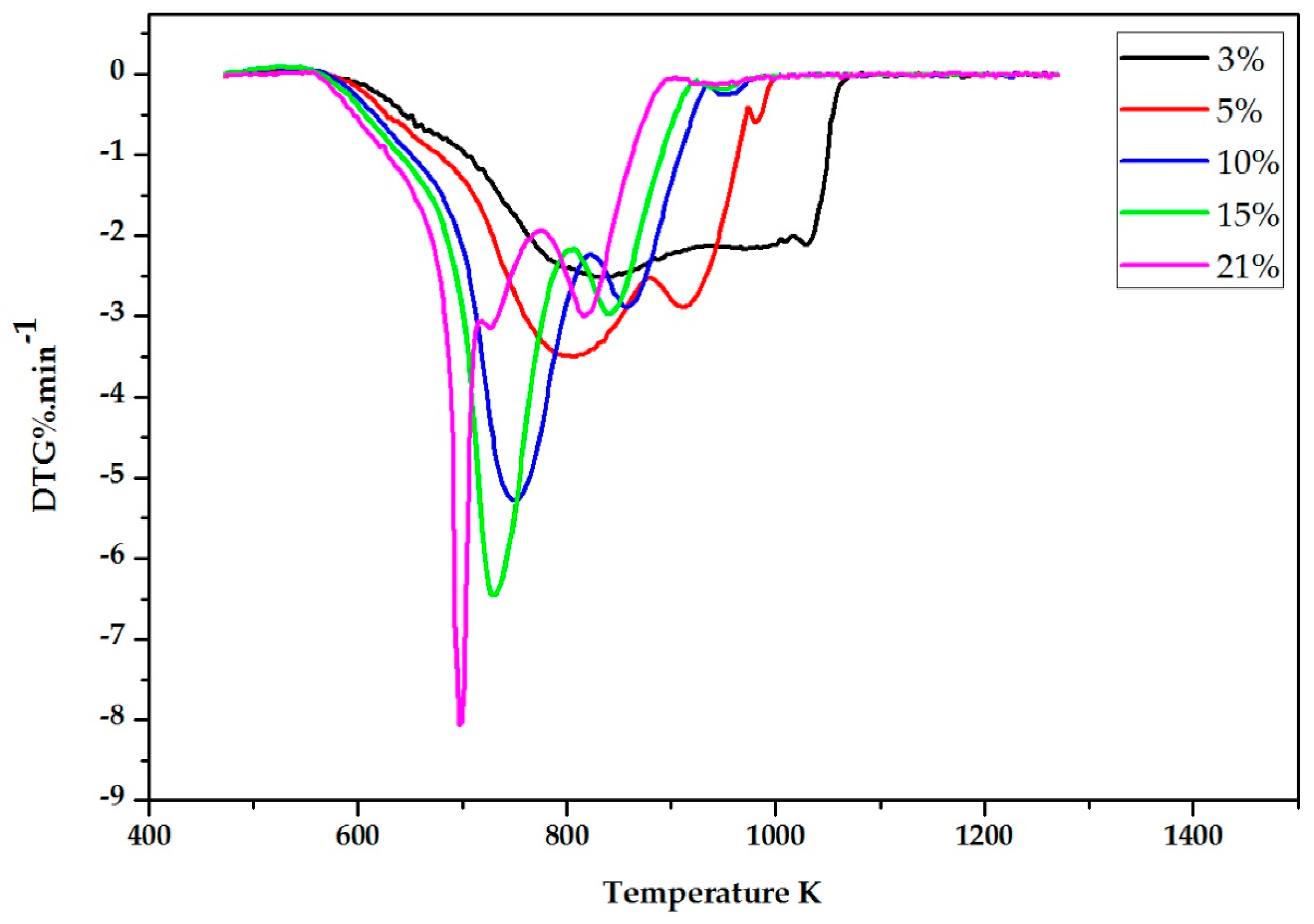
2.2. Experimental Results

The experiment of pulverized coal combustion under different O2 concentrations was conducted by TGA. During the experiment, the TGA/SDTA851e (Mettler Toledo, Zurich, Switzerland) analyzer was adopted to measure the mass loss percentage and mass loss rate of samples. Table 1 shows the proximate and ultimate analyses of Yanzhou bituminous coal.
In the experiment, the sample was initially weighted to (10 ± 0.1) mg and five samples of an equal weight were prepared. The temperature increased linearly from room temperature to 1273 K at the heating rate of 10 K·min−1. The reaction gas is the mixture of O2 and N2 with various O2 concentrations (O2 = 3%, 5%, 10%, 15%, and 21%), and the flux is kept at 30 mL·min−1.
TG and DTG (differential thermogravimetry) curves of Yanzhou pulverized coal with different O2 concentrations are described as Figure 1 and Figure 2, respectively.

3. The DIM Method Application and Discussion

The DIM method presented in Section 2.1 was applied to build the kinetic model of pulverized coal combustion under different O2 concentrations. The conversion ratio α calculated by TG data was inserted into forty-one common kinetic mechanism functions summarized as Table 2 [28,33,34].
As presented in Section 2.1, five sets of experimental data at different O2 oncentrations were used to plot ln ( β G ( α ) T T 0 ) against 1/T (Equation (11)), and then 5 × 41 sets of E values were obtained. Furthermore, 5 × 41 sets of E values were also calculated by using Equation (13). At each O2 oncentration, 41 pairs of E values from the two above-mentioned algorithms were compared for finding the closet E values. Finally, mechanism function No. 19 has the closest E values for the five sets of experimental data, and therefore it is the most probable mechanism funciton. For simplicity, 41 pairs of E values at a 10% O2 concentration were presented as an example to show the comparison of E values in Table 3.
Based on the DIM method, the most suitable kinetic mechanism function for this experiment is the Avrami-Erofeev equation with n = 4 (No. 19 in Table 2) and exhibited as:
G ( α ) = [ ln ( 1 α ) ] 4
f ( α ) = 1 4 ( 1 α ) [ ln ( 1 α ) ] 3
The calculation process of multivariable linear regression above is attained by computer programming. The estimated value of the regression coefficient β j , the confidence interval with its confidence level higher than 95% [35], and the R2 are shown as the following: β 0 = 41.040, and the confidence interval is [39.961, 42.118]; β 1   = 258,164, and the confidence interval is [250,853, 265,475]; β 2   = 3.326, and the confidence interval is [3.272, 3.380]; R2 is 0.9873.
Then, the regression model is:
y = 41.040 + 258,164 x 1 + 3.326 x 2
Therefore,   A = e 41.040 = 6.660 × 10 17   s 1 , E = 258,164 J/ mol, and n = 3.326.
A, E, n, R = 8.314 J/(mol·K) and f ( α ) are used to substitute the corresponding values in Equation (14). After rearrangement, the consequently apparent kinetic model of coal based on this experiment data is described as Equation (36).
d α / d t = 1.665 × 10 17 exp ( 31,052 / T ) ( 1 α ) [ ln ( 1 α ) ] 3 f o 2 3.326

4. Validation

The DIM method was discussed above for selecting the mechanism function and calculating the kinetic parameters. To validate the DIM method, the calculated curve using Equation (36) was compared with the experimental curve at a 7% O2 concentration ( f o 2 = 7%). The experiment of coal combustion with a 7% O2 concentration was conducted in the same conditions as the experiment aforementioned in Section 2.2. In addition, the Achar differential method [36], Coats-Redfern integral method, and the method developed by Wang et al. [14] (called the Wang method below in this paper) were respectively applied and the comparisons were provided for the prediction effect with the DIM method.
The universal Achar differential is:
ln ( d x d T f ( x ) ) = ln ( A / β ) E R T
The universal Coats-Redfern integral is:
ln ( G ( x ) T 2 ) = ln ( A R β E ) E R T
The ln ( d x d T f ( x ) ) and ln ( G ( x ) T 2 ) are separately regarded as y ; the ln ( A / β ) and ln ( A R β E ) are separately regarded as b; E R is k; and 1 T is x. Then, Equations (37) and (38) can be converted into linear equations. The plots of ln ( d x d T f ( x ) ) and ln ( G ( x ) T 2 ) vs. 1 T were drawn for each mechanism, and E values were determined by the slope after selection of the model with the biggest R2 [15,33,37].
The Wang method includes both Achar and Coats-Redfern methods. After the linear regression, two E and A are respectively obtained from the slope and intercept of the fitting curves with regard to one mechanism function. The suitable mechanism function can be judged by the closest two E values with minimum relative difference, and the relatively greater R2.
With experimental data, the forty-one sets of E, A, and R2 using Achar and Coats-Redfern are listed in Table 4. The No.19, No.19 and No.6 mechanism functions shown in Table 2 were singled out with the Achar differential method, Coats-Redfern integral method, and Wang method, respectively.
Based on the data in Table 4, the Achar method and Coats-Redfern method select the same mechanism function No. 19 shown in Table 2, but apply their own E and A. The Wang method chooses the mechanism function No. 6 shown in Table 2, but selects the E and A from the Coats-Redfern method. With the calculated E, A and the selected f ( α ) , an experimental curve and four calculated curves for the kinetic model are generated in Figure 3. Four calculated curves include the DIM method curve, Achar method curve, Coats-Redfern method curve, and Wang method curve.
Moreover, deviation is used to evaluate the accuracy of the model. The average deviation δ between the calculated and experiment curves is introduced as Equation (39) [38].
δ ( % ) = ( i = 1 N ( x i , e x p x i , c a l c ) 2 / N ) 1 / 2 max ( x i , e x p ) × 100
where δ is the average deviation; x i , e x p , x i , c a l c , and max ( x i , e x p ) respectively represent experimental values, calculated values, and the maximum experimental value; and N is the amount of experimental points. Based on Equation (39), the average deviations from different methods are calculated and shown in Table 5.
Table 5 shows that, compared with other methods, the DIM method has the lowest average deviation (1.26%), showing a good agreement with experimental observations.

5. Conclusions

The DIM method of kinetic analysis was introduced, and its application to coal combustion under different oxygen concentrations was demonstrated and validated.
  • A formula combining differential and integral was deduced through an analytical approach, which can offset the defects of a single differential or integral method.
  • In the application of the DIM method of pulverized coal combustion under different O2 concentrations (3%, 5%, 10%, 15%, and 21%), E, A, and O2 concentration exponent n were calculated as 258,164 J/mol, 6.660 × 10¹⁷ s−1, and 3.326, respectively, and the mechanism function f ( α ) was determined as the Avrami-Erofeev equation. Subsequently, the kinetic model was obtained.
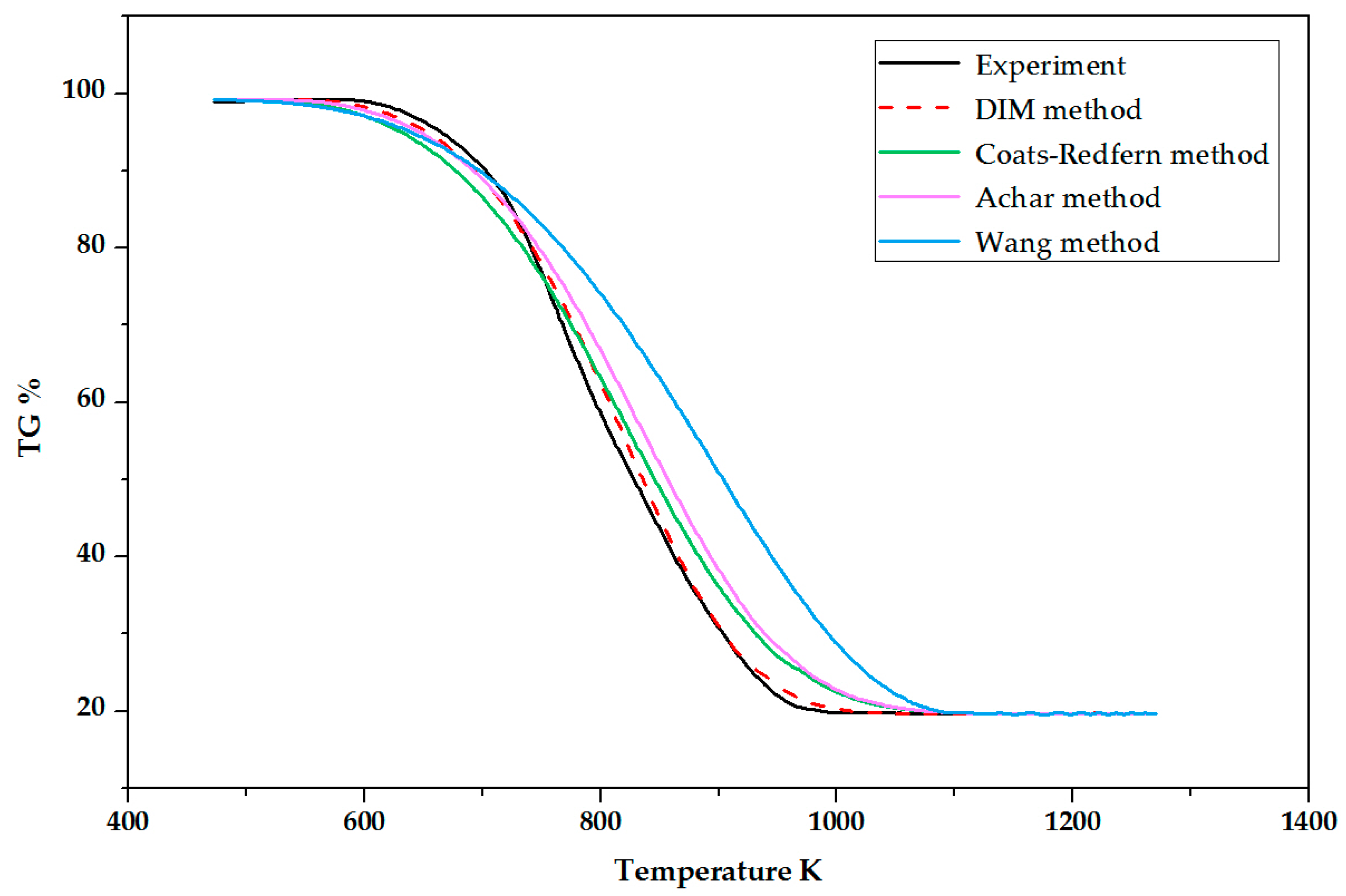
  • The experimental TG curve with a 7% O2 concentration was compared with four calculated curves generated by DIM, Wang, Achar, and Coats-Redfern methods, respectively. The DIM method showed a good accuracy with 1.26% average deviation.

Author Contributions

X.G. conceived the research. X.G. and Q.Z. carried out the experiment, deduction, and calculation. Q.Z., Y.L., Z.W., M.Z., and X.Z. participated in the analysis of the data and writing of the initial manuscript. X.G. and Q.Z. revised the manuscript and adjusted the data presentation. All authors have read and approved the manuscript.

Funding

This research was funded by the Hebei Applied Basic Research Program of China (No. 13964503D).

Conflicts of Interest

The authors declare no conflict of interest.

References

  1. Saini, V.R.; Gupta, P.; Arora, M.K. Environmental impact studies in coalfields in India: A case study from Jharia coal-field. Renew. Sustain. Energy Rev. 2016, 53, 1222–1239. [Google Scholar] [CrossRef]
  2. Saha, M.; Dally, B.B.; Medwell, P.R.; Chinnici, A. Burning characteristics of Victorian brown coal under MILD combustion conditions. Combust. Flame 2016, 172, 252–270. [Google Scholar] [CrossRef]
  3. Wang, F.F.; Li, P.F.; Mi, J.C.; Wang, J.B. A refined global reaction mechanism for modeling coal combustion under moderate or intense low-oxygen dilution condition. Energy 2018, 157, 764–777. [Google Scholar] [CrossRef]
  4. Brodny, J.; Tutak, M.; Michalak, M. The Use of the TGSP Module as a Database to Identify Breaks in the Work of Mining Machinery. In Proceedings of the 13th International Conference, Ustron, Poland, 30 May–2 June 2017. [Google Scholar]
  5. Brodny, J.; Tutak, M. Analysis of methane emission into the atmosphere as a result of mining activity. In Proceedings of the 16th International Multidisciplinary Scientific GeoConference & EXPO SGEM2016, Albena, Bulgaria, 28 June–7 July 2016. [Google Scholar]
  6. Brodny, J.; Tutak, M. Analysis of Gases Emitted into the Atmosphere during an Endogenous Fire. Available online: https://search.proquest.com/openview/8b90da3d1e86ef415620f779597cc791/1?pq-origsite=gscholar&cbl=1536338 (accessed on 5 July 2018).
  7. Pach, G.; Sułkowski, J.; Różański, Z.; Wrona, P. Costs reduction of main fans operation according to safety ventilation in mines—a case study. Arch. Mining Sci. 2018, 63, 43–60. [Google Scholar]
  8. Adamczyk, W.P.; Bialecki, R.A.; Ditaranto, M.; Haugen, N.E.L.; Katelbach-Wozniak, A.; Klimanek, A.; Sładek, S.; Szlek, A.; Wiecel, G. A method for retrieving char oxidation kinetic data from reacting particle trajectories in a novel test facility. Fuel 2018, 212, 240–255. [Google Scholar] [CrossRef]
  9. Vyazovkin, S. Kinetic concepts of thermally simulated reactions in solid: A view from a historical perspective. Int. Rev. Phys. Chem. 2000, 19, 45–60. [Google Scholar] [CrossRef]
  10. Fletcher, T.H.; Kerstein, A.R.; Pugmire, R.J.; Solum, M.S.; Grant, D.M. Chemical percolation model for devolatilization. 3. direct use of 13C NMR data to predict effects of coal type. Energy Fuels 1992, 6, 414–431. [Google Scholar]
  11. Shurtz, R.C.; Fletcher, T.H. Coal Char-CO2 Gasification Measurements and Modeling in a Pressurized Flat-Flame Burner. Energy Fuels 2013, 27, 3022–3038. [Google Scholar] [CrossRef]
  12. Niksaa, S.; Liua, G.S.; Hurtb, R.H. Coal conversion submodels for design applications at elevated pressures. Part I. devolatilization and char oxidation. Prog. Energy Combust. Sci. 2003, 29, 425–477. [Google Scholar] [CrossRef]
  13. Rojas, A.; Barraza, J.; Barranco, R.; Lester, E. A new char combustion kinetic model—Part 2: Empirical validation. Fuel 2012, 96, 168–175. [Google Scholar] [CrossRef]
  14. Wang, Y.F.; Song, Y.M.; Zhi, K.D.; Li, Y.; Teng, Y.Y.; He, R.X.; Liu, Q.S. Combustion kinetics of Chinese Shenhua raw coal and its pyrolysis Carbocoal. J. Energy Inst. 2017, 90, 624–633. [Google Scholar] [CrossRef]
  15. Niu, S.L.; Han, K.H.; Lu, C.M. Characteristic of coal combustion in oxygen/carbon dioxide atmosphere and nitric oxide release during this process. Energy Convers. Manag. 2011, 52, 532–537. [Google Scholar] [CrossRef]
  16. Bhatia, S.K.; Perlmutter, D.D. A random pore model for fluid-solid reactions: I. Isothermal, kinetic control. AIChE J. 1980, 26, 379–386. [Google Scholar]
  17. Bhatia, S.K.; Perlmutter, D.D. A random pore model for fluid-solid reactions: II. Diffusion and transport effects. AIChE J. 1981, 27, 247–254. [Google Scholar]
  18. Shao, J.G.; Zhang, J.L.; Wang, G.; Wang, Z.; Guo, H.W. Combustion Property and Kinetic Modeling of Pulverized Coal Based on Non-isothermal Thermogravimetric Analysis. J. Iron Steel Res. Int. 2014, 21, 1002–1008. [Google Scholar]
  19. Liu, Q.R.; Hu, H.Q.; Zhou, Q.; Zhu, S.W.; Chen, G.H. Effect of inorganic matter on reactivity and kinetics of coal pyrolysis. Fuel 2004, 83, 713–718. [Google Scholar] [CrossRef]
  20. Zhou, L.; Luo, T.; Huang, Q. Co-pyrolysis characteristics and kinetics of coal and plastic blends. Energy Convers. Manag. 2009, 50, 705–710. [Google Scholar] [CrossRef]
  21. Irfan, M.F.; Arami-Niya, A.; Chakrabarti, M.H.; Daud, W.M.A.W.; Usman, M.R. Kinetics of gasification of coal, biomass and their blends in air (N2/O2) and different oxy-fuel (O2/CO2) atmospheres. Energy 2012, 37, 665–672. [Google Scholar] [CrossRef]
  22. Das, T.; Baruah, B.P.; Saikia, B.K. Thermal behaviour of low-rank Indian coal fines agglomerated with an organic binder. J. Therm. Anal. Calorim. 2016, 126, 435–446. [Google Scholar] [CrossRef]
  23. Islam, A.; Auta, M.; Kabir, G.; Hameed, B.H. A thermogravimetric analysis of the combustion kinetics of karanja (Pongamia pinnata) fruit hulls char. Bioresour. Technol. 2016, 200, 335–341. [Google Scholar] [CrossRef] [PubMed]
  24. Gai, C.; Liu, Z.G.; Han, G.H.; Peng, N.N.; Fan, A.N. Combustion behavior and kinetics of lowlipid microalgae via thermogravimetric analysis. Bioresour. Technol. 2015, 181, 148–154. [Google Scholar] [CrossRef] [PubMed]
  25. Morin, M.; Pécate, S.; Masi, E.; Hémati, M. Kinetic study and modelling of char combustion in TGA in isothermal conditions. Fuel 2017, 203, 522–536. [Google Scholar] [CrossRef]
  26. Feng, S.D.; Li, P.; Liu, Z.Y.; Zhang, Y.; Li, Z.M. Experimental study on pyrolysis characteristic of coking coal from Ningdong coalfield. J. Energy Inst. 2018, 91, 233–239. [Google Scholar] [CrossRef]
  27. Duan, W.J.; Yu, Q.B.; Xie, H.Q.; Qin, Q. Pyrolysis of coal by solid heat carrier-experimental study and kinetic modeling. Energy 2017, 135, 317–326. [Google Scholar] [CrossRef]
  28. Alvarez, A.; Pizarro, C.; Garcia, R.; Bueno, J.L.; Lavin, A.G. Determination of kinetic parameters for biomass combustion. Bioresour. Technol. 2016, 216, 36–43. [Google Scholar] [CrossRef] [PubMed] [Green Version]
  29. Hu, R.Z.; Yang, Z.Q.; Liang, Y.J. The determination of the most probable mechanism function and three kinetic parameters of exothermic decomposition reaction of energetic materials by a. Thermochim. Acta 1988, 123, 135–151. [Google Scholar]
  30. Coats, A.W.; Redfern, J.P. Kinetic parameters from thermogravimetric data. Nature 1964, 201, 68–69. [Google Scholar] [CrossRef]
  31. Norwisz, J. The kinetic equation under linear temperature increase conditions. Thermochim. Acta 1978, 25, 123–125. [Google Scholar] [CrossRef]
  32. Yan, L.B.; He, B.S.; Hao, T.Y.; Pei, X.H.; Li, X.S.; Wang, C.J.; Duan, Z.P. Thermogravimetric study on the pressurized hydropyrolysis kinetics of a lignite coal. Int. J. Hydrogen Energy 2014, 39, 7826–7833. [Google Scholar] [CrossRef]
  33. Magalhaes, D.; Kazanc, F.; Riaza, J.; Erensoy, S.; Kabakli, O.; Chalmers, H. Combustion of Turkish lignites and olive residue: Experiments and kinetic modelling. Fuel 2017, 203, 868–876. [Google Scholar] [CrossRef]
  34. Duan, W.; Yu, Q.; Wu, T.; Yang, F.; Qin, Q. The steam gasification of coal with molten blast furnace slag as heat carrier and catalyst Kinetic study. Int. J. Hydrogen Energy 2016, 41, 18995–19004. [Google Scholar] [CrossRef]
  35. Murphy, J.J.; Shaddix, C.R. Combustion kinetics of coal chars in oxygen-enriched environments. Combust. Flame 2006, 144, 710–729. [Google Scholar] [CrossRef]
  36. Achar, B.N.; Brindley, G.W.; Sharp, H. Kinetics and mechanism of dehydroxylation processes: III. Applications and limitation of dynamic methods. Proc. Int. Clay. Conf. Jerusalem 1966, 1, 67–73. [Google Scholar]
  37. Dai, C.; Ma, S.; Liu, X.; Liu, X. Study on the Pyrolysis Kinetics of Blended Coal in the Fluidized-bed Reactor. Procedia Eng. 2015, 102, 1736–1741. [Google Scholar] [CrossRef]
  38. Wang, G.W.; Zhang, J.L.; Shao, J.G.; Liu, Z.J.; Zhang, G.H.; Xu, T.; Guo, J.; Wang, H.Y.; Xu, R.S.; Lin, H. Thermal behavior and kinetic analysis of co-combustion of waste biomass/low rank coal blends. Energy Convers. Manag. 2016, 124, 414–426. [Google Scholar] [CrossRef]
Figure 1. TG curves at different O2 concentrations.
Energies 11 01799 g001
Figure 2. DTG curves at different O2 concentrations.
Energies 11 01799 g002
Figure 3. The four kinds of calculated curves (DIM, Wang, Achar, and Coats-Redfern methods) and experimental TG curve at a 7% O2 concentration.
Energies 11 01799 g003
Table 1. Proximate and ultimate analyses of Yanzhou bituminous coal.
Proximate Analysis (w%)Ultimate Analysis (w%)
MadAadVadFCadCadHadNadSadOad
4.8116.9724.5153.7162.562.620.90.4111.73
Table 2. Common mechanism functions and corresponding f( α ) and G( α ).
NumberModel G ( α ) f ( α )
1Parabolic law α 2 1 2 α 1
2Valensi equation α + ( 1 α ) ln ( 1 α ) [ ln ( 1 α ) ] 1
3Jander equation [ 1 ( 1 α ) 1 2 ] 1 2 4 ( 1 α ) 1 2 [ 1 ( 1 α ) 1 2 ] 1 2
4Jander equation [ 1 ( 1 α ) 1 2 ] 2 ( 1 α ) 1 2 [ 1 ( 1 α ) 1 2 ] 1
5Jander equation [ 1 ( 1 α ) 1 3 ] 1 2 6 ( 1 α ) 2 3 [ 1 ( 1 α ) 1 3 ] 1 2
6Jander equation [ 1 ( 1 α ) 1 3 ] 2 3 2 ( 1 α ) 2 3 [ 1 ( 1 α ) 1 3 ] 1
7G-B equation 1 2 3 α ( 1 α ) 2 3 3 2 [ ( 1 α ) 1 3 1 ] 1
8Inverse Jander equation [ ( 1 + α ) 1 3 1 ] 2 3 2 ( 1 + α ) 2 3 [ ( 1 + α ) 1 3 1 ] 1
9Z-L-T equation [ ( 1 α ) 1 3 1 ] 2 3 2 ( 1 α ) 4 3 [ ( 1 α ) 1 3 1 ] 1
10Avrami-Erofeev equation [ ln ( 1 α ) ] 1 4 4 ( 1 α ) [ ln ( 1 α ) ] 3 4
11Avrami-Erofeev equation [ ln ( 1 α ) ] 1 3 3 ( 1 α ) [ ln ( 1 α ) ] 2 3
12Avrami-Erofeev equation [ ln ( 1 α ) ] 2 5 5 2 ( 1 α ) [ ln ( 1 α ) ] 3 5
13Avrami-Erofeev equation [ ln ( 1 α ) ] 1 2 2 ( 1 α ) [ ln ( 1 α ) ] 1 2
14Avrami-Erofeev equation [ ln ( 1 α ) ] 2 3 3 2 ( 1 α ) [ ln ( 1 α ) ] 1 3
15Avrami-Erofeev equation [ ln ( 1 α ) ] 3 4 3 4 ( 1 α ) [ ln ( 1 α ) ] 1 4
16Avrami-Erofeev equation [ ln ( 1 α ) ] 3 2 2 3 ( 1 α ) [ ln ( 1 α ) ] 1 2
17Avrami-Erofeev equation [ ln ( 1 α ) ] 2 1 2 ( 1 α ) [ ln ( 1 α ) ] 1
18Avrami-Erofeev equation [ ln ( 1 α ) ] 3 1 3 ( 1 α ) [ ln ( 1 α ) ] 2
19Avrami-Erofeev equation [ ln ( 1 α ) ] 4 1 4 ( 1 α ) [ ln ( 1 α ) ] 3
20First order ln ( 1 α ) 1 α
21P-T equation ln ( α 1 α ) α ( 1 α )
22Mampel power law α 1 4 4 α 3 4
23Mampel power law α 1 3 3 α 2 3
24Mampel power law α 1 2 2 α 1 2
25Mampel power law α 1
26Mampel power law α 3 2 2 3 α 1 2
27Mampel power law α 2 1 2 α 1
28Reaction order 1 ( 1 α ) 1 4 4 ( 1 α ) 3 4
29Contracting sphere 1 ( 1 α ) 1 3 3 ( 1 α ) 2 3
30Contracting sphere 3 [ 1 ( 1 α ) 1 3 ] ( 1 α ) 2 3
31Contracting cylinder 1 ( 1 α ) 1 2 2 ( 1 α ) 1 2
32Contracting cylinder 2 [ 1 ( 1 α ) 1 2 ] ( 1 α ) 1 2
33Reaction order 1 ( 1 α ) 2 1 2 ( 1 α ) 1
34Reaction order 1 ( 1 α ) 3 1 3 ( 1 α ) 2
35Reaction order 1 ( 1 α ) 4 1 4 ( 1 α ) 3
36Second order ( 1 α ) 1 ( 1 α ) 2
37Reaction order ( 1 α ) 1 1 ( 1 α ) 2
38Two-third order ( 1 α ) 1 2 2 ( 1 α ) 3 2
39Exponent law ln α α
40Exponent law ln α 2 1 2 α
41Third order ( 1 α ) 2 1 2 ( 1 α ) 3
Table 3. The comparison of E values with the forty-one mechanism functions at a 10% oxygen concentration.
No.E1 (Equation (11)) (J/mol)E2 (Equation (13)) (J/mol)E = E1E2 (J/mol)|△E/E1||△E/E2|
161,074.6434,272.7626,801.890.43880.7820
267,418.2339,282.3228,135.910.41730.7162
310,758.323345.337412.990.68902.2159
473,246.3445,688.9627,557.380.37620.6032
512,279.785360.196919.590.56351.2909
679,332.1953,748.3925,583.800.32250.4760
77,0951.6842,817.5928,134.090.39650.6571
856,576.7731,257.3125,319.460.44750.8100
9121,550.68152,645.18−31,094.500.25580.2037
103251.611488.911762.690.54211.1839
117692.945574.962117.990.27530.3799
1211,248.848843.792405.050.21380.2719
1316,578.1213,747.042831.080.17080.2059
1425,457.4721,919.133538.340.13900.1614
1529,905.4654,607.46−2,4702.000.82600.4524
1669,879.1762,779.557099.620.10160.1131
1796,525.5487,295.809229.740.09560.1057
18149,818.28136,328.3113,489.970.09000.0990
19203,111.02185,360.8117,750.210.08740.0958
2043,224.4938,263.294961.190.11480.1297
21-99,773.33---
22−1,180.59−5138.973958.383.35290.7703
231783.35−3262.225045.572.82931.5467
247712.07491.287220.790.936314.6979
2525,499.0411,751.7713,747.270.53911.1698
2643,282.6823,012.2720,270.420.46830.8809
2761,074.6434,272.7626,801.890.43880.7820
2836,431.9524,366.9412,065.000.33120.4951
2934,627.8121,489.5913,138.220.37940.6114
3034,627.8121,489.5913,138.220.37940.6114
3131,584.8917,459.8714,125.010.44720.8090
3231,584.8917,459.8714,125.010.44720.8090
3319,113.897222.9511,890.940.62211.6463
3415,430.784848.1310,582.650.68582.1828
3512,870.073261.729608.360.74662.9458
3653,276.11137,575.97−84,299.861.58230.6128
3788,876.66160,096.95−71,220.290.80130.4449
3821,599.7763,403.38−41,803.611.93540.6593
39-−167,150.70---
40-−167,150.70---
41116,645.42285,921.15−169,275.731.45120.5920
- Denotes non-real numbers.
Table 4. E, A, and R2 of pulverized coal combustion with the forty-one mechanism functions.
No.AcharC-R
E(J/mol)A(s−1)R2E(J/mol)A(s−1)R2
127,036.206.64 × 10−40.124664,006.401.740.8560
245,189.281.29 × 10−20.337570,286.463.520.8787
3643.807.71 × 10−52.38 × 10−49439.804.70 × 10−40.6541
467,295.675.03 × 10−10.642576,091.676.190.8997
510,514.864.42 × 10−40.0751610,974.366.09 × 10−40.7347
681,770.403.980.781882,229.911.03 × 1010.9165
758,959.174.34 × 10−20.533773,785.821.680.8915
820,581.271.82 × 10−50.0756759,482.266.77 × 10−20.8436
9150,204.083.07 × 1060.9567127,852.361.34 × 1050.9415
1014,669.161.91 × 10−30.19121358.774.30 × 10−50.1610
1119,381.244.97 × 10−30.29626070.863.75 × 10−40.6956
1223,150.911.02 × 10−20.37859840.531.04 × 10−30.8091
1328,805.422.85 × 10−20.490015,495.033.67 × 10−30.8713
1438,229.581.45 × 10−10.634224,919.202.25 × 10−20.9076
1542,941.675.68 × 10−10.668229,631.295.24 × 10−20.9163
1685,350.452.67 × 1020.893872,040.065.33 × 1010.9405
17113,622.971.99 × 1040.9294100,312.584.15 × 1030.9448
18170,168.009.35 × 1070.9527156,857.622.03 × 1070.9485
19226,713.043.90 × 10110.9590213,402.658.62 × 10100.9502
2057,077.933.190.797643,767.555.79 × 10−10.9301
2118,685.983.97 × 10−20.3348---
22−40,149.713.86 × 10−80.3194−3179.50−4.03 × 10−50.3664
23−36,950.387.41 × 10−80.281019.833.62 × 10−71.46 × 10⁻⁵
24−30,551.722.31 × 10−70.20516418.482.43 × 10−40.4396
25−11,355.754.14 × 10−60.030925,614.458.70 × 10−30.7814
267840.225.56 × 10−50.013344,810.431.36 × 10−10.8354
2727,036.206.64 × 10−40.124664,006.401.740.8560
2839,969.512.69 × 10−20.560036,577.092.89 × 10−20.8970
2934,266.701.16 × 10−20.446834,726.212.52 × 10−20.8833
3034,266.703.48 × 10−20.446834,726.217.57 × 10−20.8833
3122,861.091.81 × 10−30.212731,657.091.86 × 10−20.8557
3222,861.093.63 × 10−30.212731,657.093.71 × 10−20.8557
33−79,789.431.07 × 10−110.361219,246.643.40 × 10−30.6704
34−148,223.112.09 × 10−170.494315,525.151.84 × 10−30.5838
35−216,656.803.61 × 10−230.554612,918.331.15 × 10−30.5093
36125,511.612.46 × 1060.907155,656.191.81 × 1020.6242
37125,511.612.46 × 1060.907194,048.132.46 × 1040.8625
3891,294.771.40 × 1030.920521,439.357.97 × 10−20.5146
39−49,747.695.15 × 10−80.4305---
40−49,747.691.03 × 10−70.4305---
41193,945.293.79 × 10120.8546124,089.883.12 × 1080.6658
- Denotes non-real numbers.
Table 5. Average deviation comparison of different methods.
MethodAverage Deviation ( δ , % )
DIM1.26
Wang9.58
Achar4.05
Coats-Redfern3.01

