Abstract
With plug-in hybrid electric vehicles (PHEVs), the catalyst temperature is below the light-off temperature due to reduced engine load, extended engine off period, and frequent engine on/off shifting. The conversion efficiency of a three-way catalyst (TWC) and tailpipe emissions were proven to depend heavily on the temperature of the catalyst. The existing energy management strategy (EMS) of the PHEVs focuses on the improvement of fuel efficiency and emissions based on hot engine characteristics, but neglects the effect of catalyst temperature on tailpipe emissions. This paper presents a new EMS that incorporates a catalyst thermal management method. First, an additional cost is established to implement additional constraints on catalyst temperature, and then the global cost function is created using this additional cost and the fuel consumption. Second, we find the global optimal solution using Pontryagin’s minimum principle method, which provides an optimal control policy and state trajectories. Then, based on the analysis of the optimal control policy, an engine on/off filter (eng on/off filter) is introduced to command the engine on/off shifting. This filter plays an important role in adjusting both the energy and catalyst thermal management strategy for PHEVs. Finally, a practical approach based on the eng on/off filter is developed, and a genetic algorithm is applied to optimize the time constants of this filter. Simulation results demonstrate that the proposed approach‘s fuel consumption increased slightly, but the tailpipe emissions of HC (hydrocarbons), CO (carbon monoxide) and NOx (nitrogen oxide) significantly decreased compared with the standard approach.
1. Introduction
An energy management strategy (EMS) is a crucial technology for plug-in hybrid electric vehicles (PHEVs) owing to its impact on fuel economy and emissions performance [1,2]. For PHEVs, the most direct and easiest EMS is the charge depletion–charge sustaining (CD-CS)-based energy management strategy [3] that applies a threshold to the state of charge (SOC) to control the mode change. Before the SOC reaches the predetermined threshold, the vehicle is mainly powered by the battery, which is a process called CD mode. After the SOC reaches the threshold, the vehicle is powered by the engine and the battery together, which is a process called CS mode [4,5]. As this strategy is not a blended strategy, it makes the charge deplete in the whole trip. CD-CS is not able to fully exploit the potential of the plug-in hybrid system [6]. Thus, many studies have been performed to improve the energy management of PHEVs. A variety of optimal methods, such as deterministic dynamic programming (DDP) [7,8,9,10], a two-scale dynamic programming (DP) approach [11,12], stochastic dynamic programming (SDP) [13,14,15], Pontryagin’s minimal principle (PMP) [16,17,18], approximate Pontryagin’s minimum principle (A-PMP) [19], quadratic programming (QP) [20], equivalent consumption minimum strategy (ECMS) [21,22,23], and adapt equivalent consumption minimum strategy (A-ECMS) [24,25] have been successfully applied to improve the energy management of PHEVs.
The optimality criterion of the above methods is the fuel consumption and, possibly, emissions. These methods are usually based on the assumption that the PHEV system is under thermal equilibrium. However, thermal transients in the PHEV system are even more important than in conventional engine-propelled vehicles, since the engine in PHEV systems has a longer engine off period and more engine on/off shifting. Few publications have been reported on the integration of energy and thermal management for hybrid electric vehicles. Integrating energy management strategies of PHEVs with a focus on the effect of the coolant temperature on the engine performance and the vehicle power demand was reported [26]. Padovani et al. [27] proposed a strategy including the battery thermal management for hybrid electric vehicles (HEVs) to reduce the influence of battery temperature on battery aging. In Pham et al. [28], an approach for integrated energy and battery thermal management was proposed by incorporating the battery temperature and heating and cooling power demand.
In addition to coolant and battery temperatures, the catalyst temperature also influences vehicle performance, such as low catalyst temperature worsening vehicle’s tail pipe emissions and a too high catalyst temperature causing the catalyst to sinter and quickening the catalyst aging. The emission conversion efficiency of the three-way catalyst (TWC) depends heavily on the temperature of the catalyst. To achieve high conversion efficiency, the catalyst temperature must be above the light-off temperature. Therefore, fast catalyst warm-up and catalyst temperature management are key to minimizing total tailpipe emissions. An electrical heated catalyst was applied by Kessels et al. [29] to reduce the light-off time of a hybrid vehicle. Kum et al. [30] used the dynamic programming (DP) technique to optimize energy and the catalyst temperature of PHEVs for minimum fuel consumption and tailpipe emissions. Due to the optimal control policy computed by DP being time-dependent and curse of dimensionality, it is hard for DP to optimize PHEV’s torque distribution with two-state variables in real time.
Tailpipe emissions are dominated by the catalyst temperature and its conversion efficiency. In general, the light-off temperature of a TWC is between 250 °C and 350 °C, and the normal operating temperature is between 350 °C and 800 °C. When the catalyst temperature deviates from this temperature range, its conversion efficiency is low, then tailpipe emissions worsen. As a consequence, a PMP-based EMS integrating catalyst temperature is proposed in this study. This EMS adds a penalty, also called an additional cost, for undesired catalyst temperature to the global cost function, and Pontryagin’s minimum principle method is used to find the globally optimal solution. Since this EMS adds an extra co-state after integrating catalyst temperature that causes hard calibration, an engine on/off filter is introduced to command the engine on/off (eng on/off) after analyzing the above EMS’s optimal solution. Finally, a practical approach based on the eng on/off filter is developed, and a genetic algorithm (GA) is applied to optimize the time constants of the filter.
The outline of this paper is as follows. The structure and parameters of a parallel continuously variable transmission (CVT)-based PHEV powertrain are described in Section 2. The thermal model of the engine and TWC are provided in Section 3. Then in Section 4, the optimization problem with the additional catalyst temperature constraint is formulated, and this problem is solved via Pontryagin’s minimum principle. A practical approach based on the eng on/off filter is proposed in Section 5, and the GA is applied to optimize the time constants of the filter in this section. Finally, conclusions are discussed in Section 6.
2. Structure and Parameters of the Powertrain System
This study focused on a single-shaft parallel CVT-based PHEV. Figure 1 shows the powertrain of this vehicle that includes an internal combustion engine (ICE), an integrated starter and generator motor (ISG motor), battery, clutch, a continuously variable transmission (CVT), and final drive (FD). The vehicle runs in different operating modes by controlling the state of the engine and motor and the separation and combination of the clutch. According to the state of the engine, the working mode of the vehicle can be divided into two modes: engine on mode, and engine off mode. During the engine on mode, the clutch is closed, the engine provides positive power, and the output power of the motor can be positive (driving), negative (generating), or zero (idle). During the engine off mode, the clutch is open, only the motor runs, and this mode can be subdivided into motor-driving mode and braking mode. The basic parameters of the PHEV are shown in Table 1.
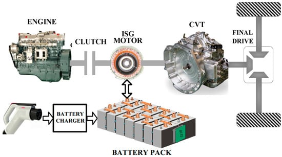
Figure 1.
Parallel continuously variable transmission (CVT)-based plug-in hybrid electric vehicle (PHEV) powertrain system.

Table 1.
Basic parameters of the PHEV.
3. Thermal Model of Engine and Three-Way Catalyst (TWC)
In this paper, the model for the supervisory control approach can be divided into two sub-models: engine thermal model and TWC thermal model. The steady-state engine model only outputs hot engine data, so establishing the engine thermal model that takes the engine’s coolant temperature into account to predict cold engine outputs is necessary, especially for engine-out emissions during cold-start. The TWC thermal model includes catalyst temperature dynamics, which are required for computing the conversion efficiency of the TWC.
3.1. Engine Thermal Model
The engine thermal model can be further divided into two sub-blocks, coolant temperature dynamics, and cold-engine correction factor. A lumped-capacitance thermal network model, depicted in Figure 2, was defined for the coolant temperature dynamics model. The heat transfer equations for calculating the coolant temperature are listed in Appendix A.
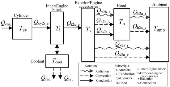
Figure 2.
Schematic illustration of the engine thermal model.
For control purposes, a simplified model that predicts cold engine outputs should be built. One approach is to simply multiply hot engine outputs by a cold factor, which is a function of the coolant temperature. This method was investigated by Murrell et al. [31], which can be expressed as follows:
where is the engine’s coolant temperature factor, is the engine cooling system’s thermostat set point, and is the coolant temperature. These temperatures are expressed in degrees centigrade. , , , and are the hot engine fuel consumption rate and hot engine outputs rate of HC, CO, and NOx, respectively. These values can be obtained by looking up maps by engine speed and engine torque, shown in Figure 3. From Figure 3a, it can be seen that fuel enriches at high speed or torque. This can be explained by looking at the fundamentals of the internal combustion engine. For the high speed or torque, the only way to increase power is to richen the mixture after the wide-open-throttle. Thus, after the wide-open-throttle, the mixture becomes richer and richer, the air/fuel ratio gets smaller and smaller and fuel efficiency is lower and lower as the required power increases. , , , and are the cold engine fuel consumption rate and cold engine outputs rate of HC, CO, and NOx, respectively; and , , , , , , , and are the curve-fitting parameters. The cold-start test data of fuel consumption and emissions are not available to the author, so above parameters come from Advanced Vehicle Simulator (ADVISOR). Their values are 1, 3.1, 7.4, 3.072, 9.4, 3.21, 0.6 and 7.3, respectively.
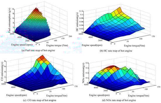
Figure 3.
The fuel consumption rate and emissions rate maps of the hot engine.
3.2. TWC Thermal Model
The schematic diagram of the TWC is shown in Figure 4. The TWC can be simplified as the catalyst monolith (A), catalyst internal shell (B), and catalyst external shell (C). The TWC thermal model uses the exhaust gas flow rate () and the exhaust gas temperature () at the TWC inlet as its inputs. The value of these inputs can be obtained by looking up maps indexed vertically by engine speed and horizontally by engine torque. The exhaust gas flow rate map, shown in Figure 5a, is available from the fuel map and air-fuel ratio (A/F) according to the following equation:
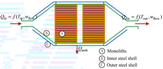
Figure 4.
Schematic diagram of the three-way catalyst (TWC).
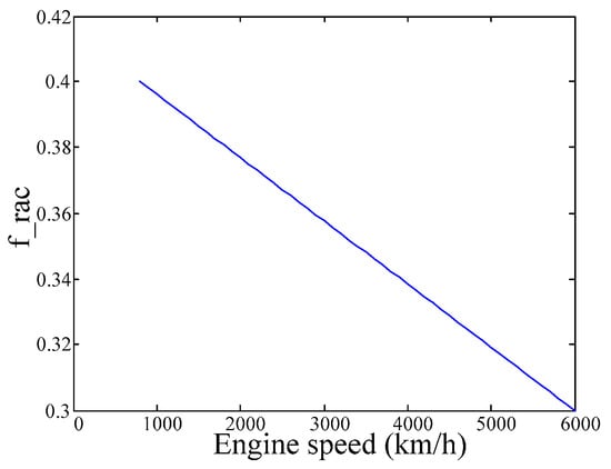
Figure 5.
The estimated value of the parameter f_rac.
The map of the exhaust gas temperature is shown in Figure 5b, which can also be obtained from the fuel map through Equations (3)–(5):
where is the engine’s waste heat, is the mass of fuel from fuel map, is the lower heating value of the fuel, is the speed of the engine with the unit of rad/s, is the engine torque, is the power of the exhaust gas, and is the fraction of waste heat that goes to the exhaust. This parameter can be estimated by engine speed, it is shown in Figure 5. is the temperature of the exhaust gas, is the exhaust gas flow with unit g/s, is the capacitance of the exhaust gas, and is the ambient temperature. It is known from Figure 6b, the exhaust gas temperature decreases with the increasing engine torque in most regions. According to Equation (5), since and are constants, the exhaust gas temperature is determined by the power of the exhaust gas and the exhaust gas flow. To explain the above phenomenon in Figure 6b, we take 3000 rpm as an example. The change curves of the exhaust gas power, flow and temperature with engine torque when engine speed is 3000 rpm are shown in Figure 7. According to this figure, when the engine torque is below 100 Nm, the exhaust gas flow’s increasing rate is greater than the rate of the exhaust gas power; therefore, the exhaust gas temperature decreases with the increasing torque in this torque range. When the engine torque is between 100 Nm and 140 Nm, the line segment AB is nearly parallel to CD, and BE is nearly parallel to DF, these mean that the exhaust gas flow’s increasing rate is nearly the same as the rate of the exhaust gas power; thus, the exhaust gas temperature is almost unchanged during this torque range. When the engine torque is above 140 Nm, the exhaust gas power’s increasing rate is obvious greater than the rate of the exhaust gas flow, so the exhaust gas temperature increases with the increasing engine torque during this torque range.
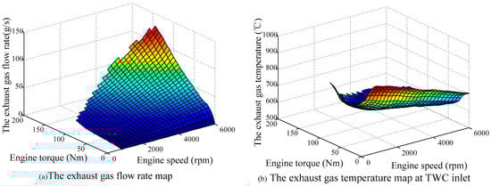
Figure 6.
Maps of the TWC inputs.
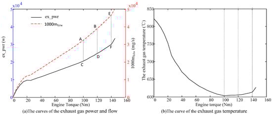
Figure 7.
The curves of the exhaust gas power, flow and temperature at 3000 rpm.
Neglecting the exhaust gas heat loss to the exhaust manifold and catalyst inlet/outlet pipes, the thermal network representing the catalyst and associated thermal elements is shown in Figure 8. The TWC was modeled through a three-node lumped capacitance model, which includes monolith (), internal shell () and external shell (). Heat is exchanged from the exhaust gas to the node of the monolith and the node of the internal shell through convection. A part of the monolith’s heat transmits to the internal shell via conduction. Heat is exchanged from the node of the internal shell to the node of the external shell via conduction and radiation. Heat transfers from the node of the external shell to the ambient air through convection and radiation. and are the resistance of thermal conduction, and are the resistance of convective heat transfer, and and are the resistance of radiative heat transfer. These thermal resistances can be obtained by the following equations:
where is thermal conductivity, is the corresponding surface area, is the representative distance between nodes, is the convective heat transfer coefficient, and are the surface temperatures, is the emissivity, and is the Steffan–Boltzman constant.
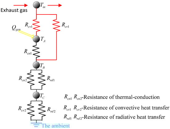
Figure 8.
Thermal network representing the catalyst and associated thermal elements.
Then, the equation for the lumped capacitor model is described as:
where is the mass of the catalyst monolith (ceramic); is the lumped thermal capacitance of the catalyst monolith is the temperature of the catalyst monolith; is the convective heat transfer coefficient between exhaust gas and catalyst monolith, which is a function of exhaust gas flow, and the function, from ADVISOR, is expressed as follows.
is the inner (honeycomb) surface area of the catalyst monolith; is the temperature of the catalyst internal shell; is the change rate of the catalyst monolith’s thermal energy; is the net heat flow from the exhaust gas to the catalyst monolith through convection; is the net heat flow from the catalyst monolith to the catalyst internal shell via conduction; is the net heat flow from chemical reactions of the exhaust gas; and , , and are the flow rates of HC, CO, and NOx in the exhaust gas, these parameters can be calculated with Equation (1). According to Equation (1), , and , also expressed as , , and , are the function of engine torque, engine speed, and the engine’s coolant temperature, while the engine’s coolant temperature is the function of the engine torque and engine speed. Therefore, these parameters are dependent on engine torque and engine speed. , , and are the molar masses of HC, CO, and NOx, respectively; , , and are the heat production of HC, CO, and NOx, respectively, by chemical reaction. , , and are the conversion efficiencies of HC, CO, and NOx, respectively. Catalyst conversion efficiencies are the function of catalyst temperature. Additionally, there is a catalyst efficiency adjustment (decrease), which is made at high exhaust flow rates. The relationship between conversion efficiency and the catalyst temperature can be described by arctan functions.
where represents each type of emission; is the light off temperature of each type of emissions; is a tuning parameter that represent a slope of the efficiency function; is a correction factor for the exhaust gas flow rate, this factor can be approximated by a linear function as shown below [32].
where is flow rate of each emission; , and are the parameters estimated by experimental data. Finally, the list of parameters is shown in Table 2.
Table 2.
Conversion efficiency model parameters.
The list of equations used for the catalyst internal shell (B) is described as follows:
where is the mass of the catalyst internal shell; is the lumped thermal capacitance of the catalyst internal shell, is the convective heat transfer coefficient between the exhaust gas and the catalyst internal shell; is the surface area of the catalyst internal shell; is the temperature of the catalyst external shell; is the change rate of the catalyst internal shell’s thermal energy; is the net heat flow from the exhaust gas to the catalyst internal shell through convection; is the net heat flow from the catalyst internal shell to the external shell via conduction and radiation; is the emissivity; and is the Stefan–Boltzmann constant .
The list of equations used for catalyst external shell (C) is as follows:
where is the mass of the catalyst external shell; is the lumped thermal capacitance of the catalyst external shell, and the value is 460 J/kgK; is the ambient temperature; is the change rate of the catalyst’s external shell’s thermal energy; is the net heat flow from the catalyst external shell to the ambient air via convection and radiation; and is the surface area of the catalyst’s external shell.
After converting the above equations, the state equation of the catalyst monolith’s temperature was obtained:
where is the engine torque and is the engine speed.
3.3. Parameter Estimation and Model Validation
We focus on parameter estimation and model validation of the engine and TWC thermal model in this section. Some of these thermal models’ parameters, shown in Table 3, are from ADVISOR, which was developed by the American National Renewable Energy Laboratory (NREL) for rapid analysis of the performance and fuel economy of conventional, electric, and hybrid vehicles and contains a component data file (its directory is “:\ADVISOR 2002\date”), this file contains several sub files, such as fuel converter data files, exhaust after treatment files, transmission data files, and driving cycle files. We can obtain the parameters in Table 3 by inspecting the fuel converter data files and exhaust after treatment files. The remaining parameters, more sensitive to coolant and catalyst temperature, come from calibration. These remaining parameters are calibrated by comparing the model’s temperature response with the test data. The parameters of the engine thermal model are tuned to match the coolant temperature responses of the model to those of the road test data, after the engine thermal model is tuned properly, parameters of the TWC model are then tuned to generate the catalyst temperature responses that match with those of road test data. Note that only limited the coolant and catalyst temperatures test data are available to the author due to the difficulty of experiment set-ups for the engine out emissions and tail out emissions, and thus, the tail-pipe emission of the model response with those of test data is not performed. The process of the real vehicle on road test and parameter estimation are shown as follows. Firstly, we chose a route in our university campus for the plug-in hybrid electric vehicle’s road testing. Then, the vehicle starts by the ISG motor. After starting, the operating mode of the vehicle was switched from pure electric mode to only engine driving mode. The signals of the vehicle speed, the engine speed, the engine torque, the coolant temperature and the catalyst temperature are collected during the test. The vehicle speed is shown in Figure 9a, and the engine torque and motor torque are shown in Figure 9b. Finally, using the vehicle speed, the engine speed, and the engine torque test data as inputs to the thermal model of engine and TWC, the parameters of the engine thermal model are tuned to match the coolant temperature responses of the model to those of the road test data, the comparison between model coolant temperature and test data temperature is shown in Figure 9c. The parameters of the TWC thermal model are tuned to match the catalyst temperature responses of the model to those of the road test data, the comparison between model catalyst temperature and test data temperature is shown in Figure 9d. The list of parameters, obtained from the tuning process, is shown in Table 4.
Table 3.
Thermal models’ parameters are from Advanced Vehicle Simulator (ADVISOR).
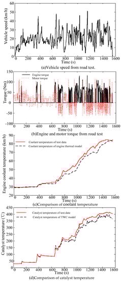
Figure 9.
Parameter estimation by matching the model’s temperature response to the test data.
Table 4.
Thermal models’ parameters determined from model tuning and validation.
After parameter estimation, another road test date is used to validate above engine and TWC thermal model. This road test’s vehicle speed is shown in Figure 10a, the engine torque and motor torque are shown in Figure 10b, the comparison between model temperature and test data temperature is shown in Figure 10c,d. From Figure 10c,d, the thermal model of the engine and TWC can predict the coolant and catalyst temperature well, despite some discrepancy existence.
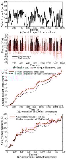
Figure 10.
Model validation by comparing model temperature with test data temperature.
4. Integrated Energy and Catalyst Thermal Management Strategy
4.1. Global Cost Function and Constraints
The energy management strategy based on optimal control theory seeks to minimize the global cost function over the total length of the trip. Most commonly, the global cost function is only the fuel consumption. However, considering some other costs in the global cost function it is possible to implement additional constraints, for example on emissions [33], drivability [34], or temperature [26]. In this paper, the proposed global cost function includes an additional cost on catalyst temperature evolution in addition to the fuel consumption, as shown in Equation (13). The constraints in this equation are the limitations of the motor, the engine, and the battery. The torque delivered by the engine has to be greater than its minimum torque and within its maximum torque, as is the case for the motor. The SOC window is limited to guarantee the performance and longevity of the battery. This study also required that the final SOC be near 0.25.
where represents the time; is the instantaneous fuel consumption that can be calculated by Equation (1); is the terminal time; is the control variable, selecting the output torque of the motor as the control variable; is the power required at the inlet of the CVT; is the torque required at the inlet of the CVT; is the vehicle speed; is the catalyst temperature; is motor’s minimum torque; is motor’s maximum torque; and are the minimum and maximum torque of the engine, respectively; and are the lower and upper limits of SOC, respectively; is a function ensuring a solution meeting the final requirement on the battery’s SOC; and is a weighting factor, which creates a trade-off between fuel consumption and the TWC’s conversion efficiency. The value of this factor is shown in Figure 11. The factor is set to 0 when the catalyst temperature is between 350 °C and 800 °C because this temperature range is a suitable temperature range for the catalyst, and the conversion efficiency of the catalyst is high at this temperature range. When the catalyst temperature exceeds 800 °C, the value of the factor increases rapidly with increasing catalyst temperature, to prevent the catalyst temperature from rising further, as an excessively catalyst temperature will cause the catalyst to sinter and quicken the catalyst aging. When the catalyst temperature is below 350 °C, the value of the factor is negative, then the additional cost is also negative, which favors catalyst warming.
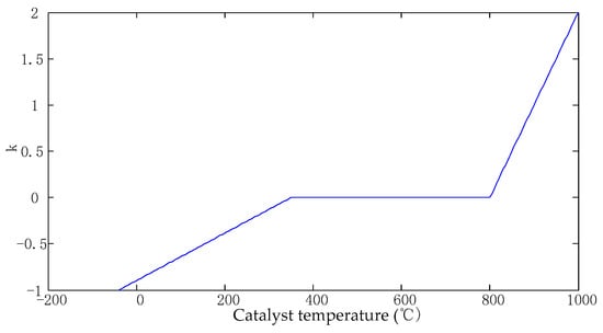
Figure 11.
The value of the weighting factor.
4.2. Establishment of the Hamilton Function
To minimize the global cost function, Pontryagin’s minimum principle (PMP) was used, and the Hamiltonian function is:
where and are the Lagrange factor, and and are the state variables, is the candidates of the control variable, or .
The simulation step size is 1 s. At t moment, .
Then, Equation (15) is expressed as follows.
The optimal control is obtained, when the following conditions are satisfied.
In Equation (16), is a constant for t moment. Thus, has no effect on Equation (17). Finally, Equation (15) is equivalent to Equation (18).
Therefore, implementing a penalty for the catalyst temperature is actually implementing a penalty for the derivative of the catalyst temperature.
The state equation of the battery‘s SOC is as follows:
where is the open circuit voltage of the battery, is the battery’s internal resistance, is the rated capacity of the battery, and is the output power of the battery.
The dynamic of the co-state on SOC is defined as:
Ignoring the impact of the battery SOC on the internal resistance and open-circuit voltage of the battery, then [35,36,37]. Therefore, .
The dynamic of the second co-state on catalyst temperature is defined as:
According to Figure 11, is equal to , 0, or , whereas , thus . From Equation (8), the Map of can be obtained, and it is shown in Figure 12.
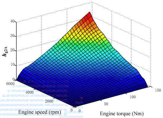
Figure 12.
The map of .
According to Figure 12, the maximum value of the is 33.67.
Equation (18) can be translated to the following equation.
According to Equation (22), we know that the Hamiltonian function is made up of three terms: the fuel consumption, equivalent fuel consumption of battery and an additional cost on catalyst temperature. Since the main tasks of the energy management system is coordination between the first two terms. The value of the additional term should be less than any remaining terms.
Figure 13 shows the change curve of the and with respect to motor torque. It can be seen that the difference between and is 4 orders of magnitude. As a consequence, if the inequality (23) is satisfied, the difference between and is at least four orders of magnitude. is obtained when PMP with the only one Lagrange factor is simulated, and the value of is about 103, Therefore, is about 10−1.
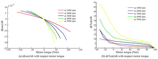
Figure 13.
The change curve of the and with respect to motor torque.
As a consequence,
Thus,
Therefore, .
4.3. Simulation Results and Discussion
The calculation process of the integrated strategy is shown in Figure 14, where is the speed of the ISG motor, is the torque required at the inlet of the CVT, is the control variable, in this paper, the control variable is the motor output torque , is the lower limit of the control variable at t moment, and is the upper limit of the control variable at t moment. The operating principle of the proposed strategy is as follows:
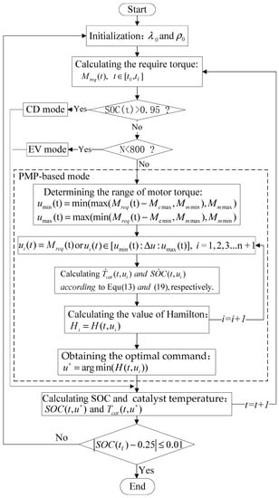
Figure 14.
The calculation process of the integrated strategy.
- (1)
- If the SOC of the battery is enough (SOC > 0.95), the vehicle works in CD mode. In this mode, the vehicle operates based on the following set of rules. If , then the torque requested can only be provided by battery; if , then the torque requested can be provided by the engine only; and if , then the engine and motor both provide the requested torque. If , then the vehicle works in mechanical braking mode.
- (2)
- If the motor speed is below the engine launch speed limit ( rpm), then the vehicle is powered entirely by the motor in electric vehicle (EV) mode.
- (3)
- If SOC ≤ 0.95 and N ≥ 800 rpm, then the optimal torque distribution is determined based on Pontryagin’s minimum principle. In other words, the vehicle works in PMP-based mode. The five steps of the optimization process under this mode are illustrated in Figure 14. The first step is determining the lower and upper limits of the control variable according to current requested torque. The second step is discretizing the control variable range (). Then, the and are calculated for every candidate control variable . The next step is the calculation of the Hamiltonian functions. The last step is comparing and obtaining the optimal command that corresponds to the smallest Hamiltonian function.
In fact, the procedure, shown in Figure 14, is known as the calibration method. It starts from an initial guess for and . The solution of the problem is then obtained by replacing at each time the value of (motor torque) resulting from the minimization Hamiltonian function. If the final value of the SOC does not match the desired terminal condition , and the engine’s catalyst has not been lighted off in all segments except for the starting stage, the value of and are adjusted until above conditions on the state is met. This approach does not yield strictly optimal results, but is more representative of what could be implemented in an actual vehicle.
To prove the significance of integrating the catalyst temperature on the PMP-based EMS of PHEVs, simulations of the integrated strategy (PMP-based with catalyst temperature) and energy-only management strategy (PMP-based without catalyst temperature) were conducted under eight repeated New European Driving Cycle (NEDC) and an urban dynamometer driving schedule/highway/urban dynamometer driving schedule (UDDS–HWFET–UDDS) driving cycle, which represents a typical work–home commute, it starts in a suburban area, characterized by environmental protection agency (EPA) urban dynamometer driving schedule (UDDS), then continues on a highway (HWFET), and finally arrives to downtown urban area, UDDS. The engine output torque and catalyst temperature trajectory are depicted in Figure 15 and Figure 16, respectively. The working points of the engine are shown in Figure 17 and Figure 18, and the fuel consumption and tailpipe emissions information is provided in Table 5.
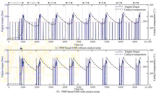
Figure 15.
Comparison of simulation results under eight repeated New European Driving Cycle (NEDC) for different energy management strategies (EMSs).
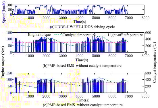
Figure 16.
Comparison of simulation results under an urban dynamometer driving schedule/highway/urban dynamometer driving schedule (UDDS–HWFET–UDDS) cycle for different energy management strategies (EMSs).
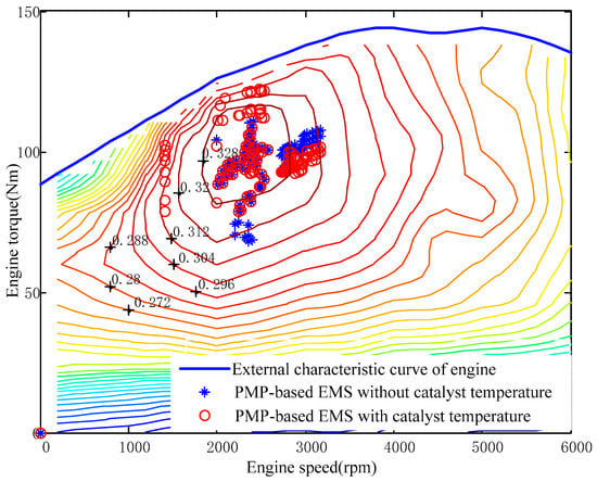
Figure 17.
Engine working points under different EMS for eight repeated NEDC cycles.
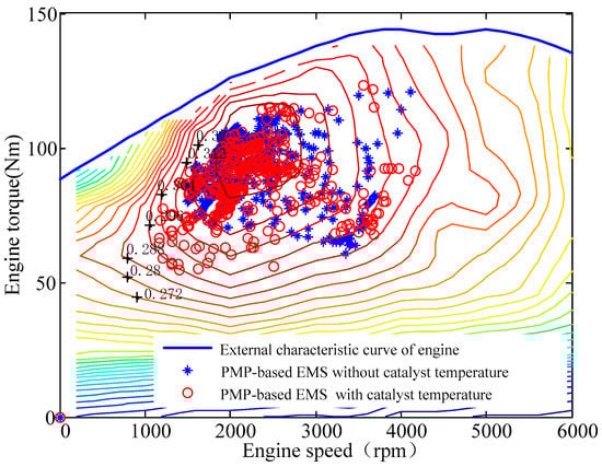
Figure 18.
Engine working points under different EMS for UDDS–HWFET–UDDS driving cycle.
Table 5.
Vehicle’s fuel consumption and tailpipe emissions under different EMSs for eight repeated NEDC cycles and UDDS–HWFET–UDDS driving cycle.
Figure 15 demonstrates the simulation results of two EMSs, PMP-based without catalyst temperature and PMP-based with catalyst temperature, over eight repeated NEDC driving cycles. The engine output torque and catalyst temperature trajectories for the PMP-based EMS without catalyst temperature are illustrated in Figure 15a. Under this strategy, the engine on/off switch is activated frequently. The light-off temperature of the catalyst is 300 °C, which is obtained from the catalyst’s product introduction. Then, as shown in Figure 15a, the catalyst has not been lighted off in the a1–a8 segments, so the tailpipe emissions will be bad. The engine output torque and catalyst temperature trajectories for the PMP-based EMS with catalyst temperature are illustrated in Figure 15b. Compared with the results of the PMP-based strategy without catalyst temperature, the number of times that the engine on/off switch is activated has been reduced significantly under the PMP-based strategy with catalyst temperature. After the engine starts, the output torque of the engine obviously increases under the condition of minimal engine efficiency loss. So, the engine’s catalyst temperature increased rapidly, and the catalyst lighted off in all segments except for b1.
Figure 16 demonstrates the simulation results of two EMSs, PMP-based without catalyst temperature and PMP-based with catalyst temperature, over a UDDS–HWFET–UDDS driving cycle. Figure 16a is the UDDS–HWFET–UDDS driving cycle. The engine output torque and catalyst temperature trajectories for the PMP-based EMS without catalyst temperature are illustrated in Figure 16b. These trajectories for the PMP-based EMS with catalyst temperature are illustrated in Figure 16c. Compared with the results of the PMP-based strategy without catalyst temperature, the number of times that the engine on/off switch is activated was reduced significantly under the PMP-based strategy with catalyst temperature. The catalyst under the EMS based on PMP without catalyst temperature did not light off most of the time, whereas the catalyst under EMS based on PMP with catalyst temperature lighted off in most segments except for the starting stages of c1 and c2.
The working points of the engine under eight repeated NEDC cycles and a UDDS–HWFET–UDDS driving cycle are shown in Figure 17 and Figure 18, respectively. Most engine working points of EMSs based on PMP without catalyst temperature and PMP with catalyst temperature are very close to each other; only a few points of the EMS based on PMP with catalyst temperature diverged from the points of the EMS based on PMP without catalyst temperature, but these points still fell within the oil economic zone.
The fuel consumption and tailpipe emissions of these EMSs are provided in Table 5. The tailpipe emissions are calculated by the following equation:
Compared with the results of the PMP-based EMS without catalyst temperature, the fuel consumption under the PMP-based EMS with catalyst temperature increased by 2.2% after eight repeated NEDC cycles, and increased by 2.27% under the UDDS–HWFET–UDDS driving cycle, but the tailpipe emissions of HC, CO, and NOx under the PMP-based EMS with catalyst temperature decreased by 17.9, 25.9, and 24.5%, respectively, under eight repeated NEDC cycles and decreased by 16.65, 24.15, and 23.88%, respectively, under the UDDS–HWFET–UDDS driving cycle. Thus, after integrating catalyst temperature in the PMP-based EMS of PHEVs, the vehicle’s tailpipe emissions were considerably reduced with minimal fuel consumption increase.
5. Real-Time Implementation
5.1. Energy Management Strategy (EMS) Based on Pontryagin’s Minimal Principle (PMP) with Eng on/off Filter
Although the PMP-based approach could be implemented in the real-time control of a vehicle, the proposed PMP with catalyst temperature strategy requires an extra co-state after integrating catalyst temperature. As PMP-based EMSs are sensitive to the co-state, PMP-based EMSs with only one co-state are difficult to calibrate, let alone PMP-based EMSs with two co-states.
According to the results, as shown in Figure 15 and Figure 16, the proposed PMP-based strategy with catalyst temperature influences the catalyst to light off by reducing the engine on/off shifting times. Based on the analysis of the optimal control policy, an engine on/off filter (eng on/off filter) was introduced to command the engine on/off shifting. The PMP-based strategy with an eng on/off filter can reduce the engine on/off shifting times without adding an extra co-state; therefore, it is easily applicable to a standard optimal online EMS.
The calculation process of the PMP-based EMS with eng on/off filter is shown in Figure 19. The engine on/off filter, without adding any control variable or co-state, can prevent the engine from experiencing frequent starts and stops, and engine on/off requests sent to the filter are basically determined by the engine torque command. If a non-zero engine torque is distributed by the control strategy, then an engine on request is prompted to the filter. Otherwise, an engine off request is sent to the filter. The filter has two time constants, s and s. The rules of the filter can be expressed as:
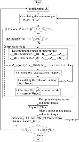
Figure 19.
Calculation process of PMP-based EMS with eng on/off filter.
- (1)
- If the engine is on and the elapsed time of the zero engine torque signal is s, then the engine off request passes through the engine on/off filter, and the engine off command will be sent to the engine plant in the next time step.
- (2)
- If the engine is on and the elapsed time of the zero engine torque signal is shorter than s, then the engine off request cannot pass through the engine on/off filter, and the engine must remain in an idle state.
- (3)
- If the engine is off and the elapsed time of the non-zero engine torque signal is s, then the engine on request passes through the engine on/off filter, and the engine on command and engine torque command will be sent to the engine plant.
- (4)
- If the engine is off and the elapsed time of the non-zero engine torque signal is shorter than s, then, the engine on request cannot pass through the engine on/off filter. In this situation, the engine torque command cannot be implemented by the engine, which is still off. So, the original torque distribution will be redistributed, and the torque originally assigned to the engine will be transferred to the ISG motor.
- (5)
- Except for the situations mentioned above, the engine will remain in its current state.
5.2. Optimization of Filter Time Constants Based on Genetic Algorithm
The filter’s time constants, s and s, considerably affect a vehicle’s fuel economy and emissions. The fuel economy is worse because and change the original optimal torque distribution from PMP-based EMS, but if the values of and are properly optimized, the engine on/off shifting times decrease, the engine works concentrated, the catalyst will warm up rapidly, and vehicle emissions will decrease considerably at the expense of a minimal fuel increase. So, optimizing these time constants is necessary. The time constant optimization problem is highly non-linear, so finding the optimal constants through analytical or numeric methods is difficult. The genetic method was introduced to effectively determine these constants. The fitness function is expressed as:
where is engine’s fuel consumption; HC, CO, and NOx are the tailpipe emissions of HC, CO, and NOx, respectively. , , , and are the maximum values of the engine’s fuel consumption and tailpipe emissions, and the fuel consumption and tailpipe emissions under the CD-CS control strategy for eight repeated NEDC driving cycles are defined as this maximum values; is the weight of the engine’s fuel consumption; and , , and are the weight of tailpipe emissions of HC, CO, and NOx, respectively.
In this paper, the parameters of and are integers, so we transform the floating point numbers of all the produced individuals to integers and then operate them on the PMP-based on EMS with eng on/off filter. The round function is used for rounding individuals to the nearest integer. The parameters of the algorithm were set as follows. The maximum iteration of the genetic method was 80, the population size was 100, the crossover probability was 0.7, and the mutation probability was 0.01. The optimization result is shown in Figure 20. With the continuous evolution of the population, the fitness function value decreased, and this value converged to 2.5269, and its corresponding best individual was (,) = (5,2). Since the best individual is optimized for a given driving cycle, this individual may not suit for another velocity profile. In practical applications, we can optimize these parameters of and under different driving cycles, driving distances, and initial battery SOC off-line, then, a compromise value can be chosen as the final value.
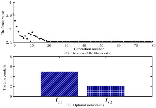
Figure 20.
The optimization result obtained with a genetic algorithm (GA).
5.3. Simulation Results of PMP-Based EMS with Eng on/off Filter
To validate the effect of the real-time EMS based on PMP with eng on/off filter, three EMSs were simulated under eight repeated NEDC driving cycles and a UDDS–HWFET–UDDS driving cycle. These EMSs included a PMP-based EMS without catalyst temperature, a PMP-based EMS with catalyst temperature and a PMP-based EMS with eng on/off filter. The simulation results are depicted in Figure 21 and Figure 22, and the fuel consumption and tailpipe emissions information are provided in Table 6 and Table 7, respectively.
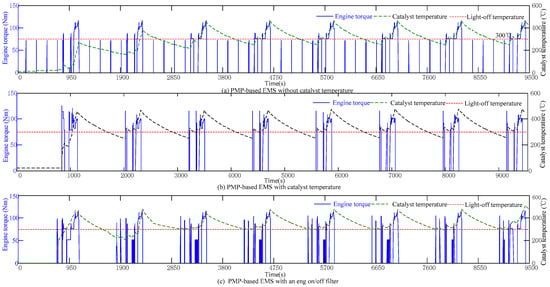
Figure 21.
The simulation results under different EMSs for eight repeated NEDC cycles.
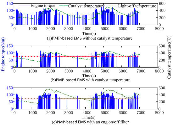
Figure 22.
Simulation results under different EMSs for the UDDS–HWFET–UDDS driving cycle.
Table 6.
Vehicle’s fuel consumption and tailpipe emissions under different EMSs for eight repeated NEDC cycles.
Table 7.
Vehicle’s fuel consumption and tailpipe emissions under different EMSs for the UDDS–HWFET–UDDS driving cycle.
Figure 21 outlines the simulation results under the three control strategies for eight repeated NEDC driving cycles. According to the figure, under PMP-based EMS without catalyst temperature, the engine starts and stops frequently, and the engine’s working time is dispersed. The catalyst does not light off for most of the time, so the efficiency of the catalytic converter is low. under the PMP-based EMS with catalyst temperature and the PMP-based EMS with an eng on/off filter, the engine on/off shifting times decreased considerably, the engine’s working time concentrated, the engine’s catalyst temperature increased rapidly, and the catalyst lighted off in most segments except for the starting stage.
Table 6 is the engine’s fuel consumption and tailpipe emissions of the three EMSs under eight repeated NEDC driving cycles. Compared with the results of the PMP-based EMS with catalyst temperature, the fuel consumption, and HC, CO, and NOx emissions under the PMP-based EMS with an eng on/off filter increased by 0.8%, 5.33%, 5.45%, and 4.73%, respectively. However, compared with the results of the PMP-based EMS without catalyst temperature, the tailpipe emissions of HC, CO, and NOx under PMP-based EMS with an eng on/off filter decreased by 13.57%, 21.9%, and 20.99%, respectively, with the fuel consumption only increasing by 3%.
Figure 22 outlines the simulation results under the three control strategies for the UDDS–HWFET–UDDS driving cycle. Figure 22a–c are the change curves of the engine torque and catalyst temperature under the different EMSs. According to the figure, the catalyst under the PMP-based EMS without catalyst temperature does not light off for the majority of the time, whereas the catalyst under the PMP-based EMS with catalyst temperature and the PMP-based EMS with an eng on/off filter lighted off in most segments except for the starting stage. This is because the engine under the PMP-based EMS without catalyst temperature starts and stops frequently, and the engine’s working time is dispersed. However, under the PMP-based EMS with catalyst temperature and the PMP-based EMS with an eng on/off filter, the engine on/off shifting times obviously decreased, the engine’s working time concentrated, and the engine’s catalyst temperature increased rapidly.
Table 7 provides the engine’s fuel consumption and tailpipe emissions of the three EMSs under the UDDS–HWFET–UDDS driving cycle. Compared with the results of the PMP-based EMS with catalyst temperature, the fuel consumption, HC emissions, CO emissions and NOx emissions under the PMP-based EMS with an eng on/off filter increased by 1.62%, 6.06%, 6.26%, and 4.84%, respectively. However, compared with the results of the PMP-based EMS without catalyst temperature, the tailpipe emissions of HC, CO, and NOx under the PMP-based EMS with an eng on/off filter, decreased by 11.59%, 19.4%, and 20.19%, respectively, with the fuel consumption only increasing by 3.92%.
From above analysis, we concluded that the HC, CO, and NOx emissions of the proposed real-time PMP-based approach with eng on/off filter significantly decreased with a slight fuel consumption increase, compared with the standard PMP-based EMS without catalyst temperature.
6. Conclusions
The catalyst temperature has an important effect on the conversion efficiency of a three-way catalyst and vehicle tailpipe emissions. Therefore, the PMP-based EMS with catalyst temperature considered a soft constraint, also called an additional cost, on the catalyst temperature, and added the additional cost to the global cost function to be minimized. The problem was solved using Pontryagin’s minimum principle, Our EMS significantly reduced the number of engine starts and stops times, enabled the rapid warmup of the catalyst, and greatly reduced the tailpipe emissions with an only slight fuel consumption increase. However, this EMS adds a co-state after integrating the catalyst temperature, which restricts its application in real-time control.
To solve the above problem, we introduced an engine on/off filter to command the engine on/off shifting. Based on the eng on/off filter, a real-time PMP-based EMS with eng on/off filter was developed, and a genetic algorithm was applied to optimize the time constants of the filter. To validate the effect of the real-time PMP-based EMS with an eng on/off filter, we simulated three EMSs under eight repeated NEDC driving cycles and a UDDS–HWFET–UDDS driving cycle. Simulation results demonstrated that the fuel consumption of our proposed approach slightly increased, but the tailpipe emissions of HC, CO, and NOx significantly decreased compared to the standard PMP-based approach without catalyst temperature.
Currently, the proposed strategy has only been verified through simulations. The next step would be to perform hardware-in-the-loop tests or experimental validations.
Author Contributions
Y.Z. wrote the paper and provided algorithms; Y.C. and C.C. built the simulation model and completed the simulation for different EMSs; and G.K. and W.G. analyzed the simulation results.
Funding
This research was funded by the National Natural Science Foundation of China (Grant No. 51665020) and the state key laboratory of mechanical transmission’s open fund (Grant No. SKLMT-KFKT-201617).
Conflicts of Interest
The authors declare no conflict of interest.
Abbreviations
The following abbreviations are used in this manuscript:
| PHEVs | plug-in hybrid electric vehicles |
| TWC | three-way catalyst |
| CVT | continuously variable transmission |
| ICE | engine |
| ISG | motor integrated starter and generator motor |
| A | the catalyst monolith |
| B | catalyst internal shell |
| C | catalyst external shell |
| i | inner/engine block |
| x | exterior/engine accessories |
| cy | cylinder |
| h | engine hood |
| EMS | energy management strategy |
| PMP | pontryagin’s minimum principle |
| DP | dynamic programming |
| ECMS | equivalent consumption minimum strategy |
| GA | genetic algorithm |
| eng on/off | engine on/off |
| SOC | state of charge |
| CD | charge depleting |
| CS | charge sustaining |
| EV | electric vehicle |
| NEDC | the new european driving cycle |
| UDDS | environmental protection agency (EPA) urban dynamometer driving schedule |
| HWFET | EPA highway fuel economy test cycle |
Appendix A. List of Equations Used for Engine Thermal Model
References
- Kim, N.; Cha, S.; Peng, H. Optimal equivalent fuel consumption for hybrid electric vehicles. IEEE Trans. Veh. Technol. 2012, 20, 817–825. [Google Scholar]
- Kim, N.; Cha, S.; Peng, H. Optimal control of hybrid electric vehicles based on Pontryagin’s minimum principle. IEEE Trans. Veh. Technol. 2011, 19, 1279–1287. [Google Scholar]
- Guzzella, L.; Sciarretta, A. Control of hybrid electric vehicles: Optimal energy management strategies. IEEE Control Syst. Mag. 2007, 27, 60–70. [Google Scholar]
- Chen, Z.; Xia, B.; You, C.; Mi, C.C. A novel energy management method for series plug-in hybrid electric vehicles. Appl. Energy 2015, 145, 172–179. [Google Scholar] [CrossRef]
- Overington, S.; Rajakaruna, S. High-efficiency control of internal combustion engines in blended charge depletion/charge sustenance strategies for plug-in hybrid electric vehicles. IEEE Trans. Veh. Technol. 2015, 64, 48–61. [Google Scholar] [CrossRef]
- Wirasingha, S.G.; Emadi, A. Classification and review of control strategies for plug-in hybrid electric vehicles. IEEE Trans. Veh. Technol. 2011, 60, 111–122. [Google Scholar] [CrossRef]
- Gong, Q.; Li, Y.; Peng, Z.R. Computationally efficient optimal power management for plug-in hybrid electric vehicles with spatial domain dynamic programming. In Proceedings of the ASME 2008 Dynamic Systems and Control Conference, Ann Arbor, MI, USA, 20–22 October 2008. [Google Scholar]
- Zou, Y.; Liu, T.; Sun, F.C.; Peng, H. Comparative study of dynamic programming and Pontryagin’s minimum principle on energy management for a parallel hybrid electric vehicle. Energies 2013, 6, 2305–2318. [Google Scholar]
- Chen, Z.; Mi, C.C.; Xu, J.; Gong, X.Z.; You, C.W. Energy management for a power-split plug-in hybrid electric vehicle based on dynamic programming and neural networks. IEEE Trans. Veh. Technol. 2014, 63, 1567–1580. [Google Scholar] [CrossRef]
- Wang, X.; He, H.; Sun, F.; Zhang, J. Application study on the dynamic programming algorithm for energy management of plug-in hybrid electric vehicles. Energies 2015, 8, 3225–3244. [Google Scholar] [CrossRef]
- Gong, Q.; Li, Y.; Peng, Z.R. Trip based power management of plug-in hybrid electric vehicle with two-scale dynamic programming. In Proceedings of the Vehicle Power and Propulsion Conference (VPPC 2007), Arlington, TX, USA, 9–12 September 2007. [Google Scholar]
- Gong, Q.; Li, Y.; Peng, Z.R. Computationally efficient optimal power management for plug-in hybrid electric vehicles based on spatial-domain two-scale dynamic programming. In Proceedings of the 2008 IEEE International Conference on Vehicular Electronics and Safety (ICVES 2008), Columbus, OH, USA, 22–24 September 2008. [Google Scholar]
- Moura, S.J.; Callaway, D.S.; Fathy, H.K.; Stein, J.L. Tradeoffs between battery energy capacity and stochastic optimal power management in plug-in hybrid electric vehicles. J. Power Source 2010, 195, 2979–2988. [Google Scholar] [CrossRef]
- Wu, X.; Hu, X.; Moura, S.; Yin, X.; Pickert, V. Stochastic control of smart home energy management with plug-in electric vehicle battery energy storage and photovoltaic array. J. Power Source 2016, 333, 203–212. [Google Scholar] [CrossRef]
- Wu, X.; Hu, X.; Yin, X.; Moura, S. Stochastic Optimal Energy Management of Smart Home with PEV Energy Storage. IEEE Trans. Smart Grid 2016, 7, 1–11. [Google Scholar] [CrossRef]
- Xu, L.; Ouyang, M.; Li, J.; Yang, F.; Lu, L.; Hua, J. Application of Pontryagin’s Minimal Principle to the energy management strategy of plugin fuel cell electric vehicles. Int. J. Hydrogen Energy 2013, 38, 10104–10115. [Google Scholar] [CrossRef]
- Chen, Z.; Mi, C.C.; Xia, B.; You, C. Energy management of power-split plug-in hybrid electric vehicles based on simulated annealing and Pontryagin’s minimum principle. J. Power Source 2014, 272, 160–168. [Google Scholar] [CrossRef]
- Onori, S.; Tribioli, L. Adaptive Pontryagin’s Minimum Principle supervisory controller design for the plug-in hybrid GM Chevrolet Volt. Appl. Energy 2015, 147, 224–234. [Google Scholar] [CrossRef]
- Hou, C.; Ouyang, M.; Xu, L.; Wang, H. Approximate Pontryagin’s minimum principle applied to the energy management of plug-in hybrid electric vehicles. Appl. Energy 2014, 115, 174–189. [Google Scholar] [CrossRef]
- Chen, Z.; Mi, C.C.; Xiong, R.; Xu, J.; You, C. Energy management of a power-split plug-in hybrid electric vehicle based on genetic algorithm and quadratic programming. J. Power Source 2014, 248, 416–426. [Google Scholar] [CrossRef]
- Gao, A.; Deng, X.; Zhang, M.; Fu, Z.M. Design and Validation of Real-Time Optimal Control with ECMS to Minimize Energy Consumption for Parallel Hybrid Electric Vehicles. Math. Probl. Eng. 2017, 2017. [Google Scholar] [CrossRef]
- Geng, B.; Mills, J.K.; Sun, D. Energy management control of microturbine-powered plug-In hybrid electric vehicles using the telemetry equivalent consumption minimization Strategy. IEEE Trans. Veh. Technol. 2011, 60, 4238–4248. [Google Scholar] [CrossRef]
- Nüesch, T.; Cerofolini, A.; Mancini, G.; Cavina, N.; Onder, C.; Guzzella, L. Equivalent consumption minimization strategy for the control of real driving NOx emissions of a diesel hybrid electric vehicle. Energies 2014, 7, 3148–3178. [Google Scholar] [CrossRef]
- Montazeri-Gh, M.; Pourbafarani, Z. Near-Optimal SOC Trajectory for Traffic-based Adaptive PHEV Control Strategy. IEEE Trans. Veh. Technol. 2017, 66, 9753–9760. [Google Scholar] [CrossRef]
- Han, J.; Park, Y.; Kum, D. Optimal adaptation of equivalent factor of equivalent consumption minimization strategy for fuel cell hybrid electric vehicles under active state inequality constraints. J. Power Source 2014, 267, 491–502. [Google Scholar] [CrossRef]
- Lescot, J.; Sciarretta, A.; Chamaillard, Y.; Charlet, A. On the integration of optimal energy management and thermal management of hybrid electric vehicles. In Proceedings of the Vehicle Power and Propulsion Conference (VPPC), Lille, France, 1–3 September 2010. [Google Scholar]
- Padovani, T.M.; Debert, M.; Colin, G.; Yann, C. Optimal energy management strategy including battery health through thermal management for hybrid vehicles. IFAC Proc. Vol. 2013, 46, 384–389. [Google Scholar] [CrossRef]
- Pham, H.T.; Van, P.P.J.; Kessels, J.; Huisman, R.G.M. Integrated energy and thermal management for hybrid electric heavy duty trucks. In Proceedings of the Vehicle Power and Propulsion Conference (VPPC), Seoul, Korea, 9–12 October 2012. [Google Scholar]
- Kessels, J.T.B.A.; Foster, D.L.; Bleuanus, W.A.J. Towards integrated powertrain control: Thermal management of NG heated catalyst system. In Proceedings of the Les Rencontres Scientifiques de l’IFP-Advances in Hybrid Powertrains, Rueil-Malmaison, France, 25–26 November 2008. [Google Scholar]
- Kum, D.; Peng, H.; Bucknor, N.K. Optimal Energy and Catalyst Temperature Management of Plug-in Hybrid Electric Vehicles for Minimum Fuel Consumption and Tailpipe Emissions. IEEE Trans. Control Syst. Technol. 2012, 21, 14–26. [Google Scholar] [CrossRef]
- Murrell, J.D.; Lewis, G.M.; Baker, D.M.; Assanis, D.N. An Early-Design Methodology for Predicting Transient Fuel Economy and Catalyst-Out Exhaust Emissions; SAE Technical Paper; SAE: Warrendale, PA, USA, 1997. [Google Scholar] [CrossRef]
- Sanketi, P.R.; Hedrick, J.K.; Kaga, T. A simplified catalytic converter model for automotive cold-start control applications. In Proceedings of the International Mechanical Engineering Congress and Exposition 2005, Orlando, FL, USA, 5–11 November 2005. [Google Scholar]
- Michel, P.; Charlet, A.; Colin, G.; Yann, C.; Nouillant, C.; Bloch, G. Energy management of HEV to optimize fuel consumption and pollutant emissions. In Proceedings of the 2012 International Symposium on Advanced Vehicle Control, Seoul, Korea, 10–12 September 2012. [Google Scholar]
- Debert, M.; Padovani, T.M.; Colin, G.; Chamaillard, Y.; Guzzella, L. Implementation of comfort constraints in dynamic programming for hybrid vehicle energy management. Int. J. Veh. Des. 2012, 58, 367–386. [Google Scholar] [CrossRef]
- Serrao, L.; Onori, S.; Rizzoni, G. A comparative analysis of energy management strategies for hybrid electric vehicles. J. Dyn. Syst. Meas. Control 2011, 133, 031012. [Google Scholar] [CrossRef]
- Tribioli, L.; Onori, S. Analysis of energy management strategies in plug-in hybrid electric vehicles: Application to the GM Chevrolet Volt. In Proceedings of the American Control Conference, Washington, DC, USA, 17–19 June 2013. [Google Scholar]
- Sharma, O.P.; Onori, S.; Guezennec, Y. Analysis of Pontryagin’s minimum principle-based energy management strategy for phev applications. In Proceedings of the ASME 2012 5th Annual Dynamic Systems and Control Conference joint with the JSME 2012 11th Motion and Vibration Conference, Fort Lauderdale, FL, USA, 17–19 October 2012. [Google Scholar]
© 2018 by the authors. Licensee MDPI, Basel, Switzerland. This article is an open access article distributed under the terms and conditions of the Creative Commons Attribution (CC BY) license (http://creativecommons.org/licenses/by/4.0/).