1. Introduction
Currently, there is an exponential growth of technological developments in the fields of electric vehicles (EVs), hybrid electric vehicles (HEVs), plug-in electric vehicles (PEVs), and other automotive applications. Due to the long-life cycle, high energy density, and low self-discharge rate, lithium-ion batteries are used as a highly prospective technology. The state of charge (SOC) is a critical factor which affects the safe and reliable operation of the battery. Typically, a battery pack used for a vehicular application comprises several hundreds of cells, which are connected in series and in parallel, in order to meet the voltage and power requirements of the application. In such a case, the state information of each cell is very important due to the potential risk of a string of batteries failing to supply the power to the vehicle if any battery cell in a string becomes faulty. Various approaches such as Coulomb counting, fuzzy logic (FL), artificial neural networks (ANNs), and Kalman filters were applied for online SOC estimation of batteries [
1,
2,
3,
4,
5]. The Coulomb-counting method which measures the amount of charge withdrawn from or put into the battery in terms of ampere hours is simple, and it requires low computing power. However, the initial SOC of the battery must be known for the start-up of SOC estimation. Furthermore, recalibration is required when the counting of ampere hours is performed over a long period of time, since the significant error in SOC estimation occurs due to an accumulation of errors in the measurement process. The ANN and FL approaches can estimate the SOC of a battery with an arbitrary initial SOC value [
6,
7]. The robustness of these models strongly relies on the quantity and quality of the training dataset. A limited training dataset may result in limited model robustness, thereby reducing the applicability of the method [
8,
9,
10]. The extended Kalman filter (EKF) approach is a computationally efficient, recursive, digital signal processing technique that was designed to remove unwanted noise from data, and is used to estimate the state of nonlinear dynamic systems. The EKF predicts a new state and its instability, before correcting the new measurement by minimizing the mean-squared error [
11,
12]. However, in commercial electric vehicle applications, the power supply of these engines requires battery packs that consist of hundreds of cells, consequently limiting the use of these algorithms due to their complexity. Highly accurate SOC information of multiple batteries is, therefore, essential for such a scenario. Moreover, accurate information on the battery impedance based on the equivalent circuit model (ECM) is extremely important and necessary for battery SOC estimation [
13,
14]. However, a complex estimation algorithm for individual cells in a module would lead to computational overkill, and would not be appropriate for implementation in a low-cost microcontroller commercially available in the market [
13]. Hence, variation in impedance must be accurately determined under various operating conditions, and over the battery’s lifetime, together with its dependence on current, SOC, temperature, and aging [
14]. Notable analyses of the effect of variable temperature and aging under actual drive cycles on the performance of lithium-ion battery modules for an electric vehicle can be found in References [
15,
16]. In addition, to obtain data for this variation, many experiments are required that are not only time-consuming, but also labor intensive.
Typically, a battery module for vehicular applications comprises hundreds of cells that are connected in series and parallel combinations to provide high power to the load. SOC imbalance may occur due to individual cell characteristics, such as capacity, SOC, temperature, and aging, as previously mentioned. Thus, a battery management system (BMS) is often adopted for managing the SOCs of battery cells in a module, as any imbalance among battery cells contributes to a reduction in capacity of the battery module, which may severely deteriorate its performance and cause early failure. The imbalance among cells in a battery pack can be caused by several factors, either extrinsic or intrinsic to the cell’s properties [
17]. Extrinsic factors include current variations in parallel strings, or voltage variations in series strings, as well as environmental storage conditions which lead to an imbalance in the extent of the cell’s reaction. Intrinsic factors include variations in cell quality caused by variations in the content of the active material, composition, and physical property of the cells. The effects of cell imbalance can be summarized by three effects. Firstly, overvoltage exposure leads to faster cell degradation, as once a cell has a lower capacity, it is exposed to a higher voltage during charge. Thus, degradation of the cell accelerates and its capacity further reduces, resulting in thermal runaway. Secondly, overcharging and overheating cause chemical reaction hazards between the active components and with the electrolyte, ultimately leading to explosions or fires. If one cell is deteriorated, it can initiate an explosive chain reaction for other cells. Thirdly, the charging or discharging period of deteriorated cells is much quicker than usual due to safety protections, thereby reducing the capacity of the battery pack. The charging process is terminated if one of the cells exceeds the charge cut-off voltage, so as to prevent overcharging. Similarly, termination of the discharging process occurs when any of the cells reach the discharge voltage threshold. Therefore, the SOC of the individual cell in a battery module needs to be estimated accurately, in combination with the cell-balancing process, to keep the energy of the cells balanced, and to extend their lifetimes.
In this paper, a simple SOC estimation method suitable for multiple cells is proposed using a nonlinear state observer (NSO). In order to reduce computational burden, the complex cell impedance was simplified to an ohmic resistance, and a ratio vector was used to reflect the relative variation in impedance with respect to each cell in the module. Furthermore, online parameter identification for the lithium-ion (Li-ion) batteries was included using an autoregressive exogenous (ARX) model, so as to achieve robust SOC estimation without any pretests for parameter identification under variations in temperature. As the process included SOC estimation of multiple battery cells, the computational burden was a very important design consideration for the reduction of overall system cost. Therefore, the NSO was preferred due to its lower computation burden and better performance for multi-cell applications [
18].
All details on the proposed method are given in the sections below. In
Section 2, the simplified battery model used for SOC estimation is discussed. In
Section 3, the ARX-based model and online parameter identification method using a recursive least square (RLS) algorithm is introduced. SOC estimation using a nonlinear state observer is presented in
Section 4, and its superiority with respect to the linear observer was verified. In
Section 5, SOC estimation of multiple cells using a nonlinear state observer is discussed. Finally, the performance of the proposed algorithm was verified using experimental results in
Section 6.
2. Battery Model
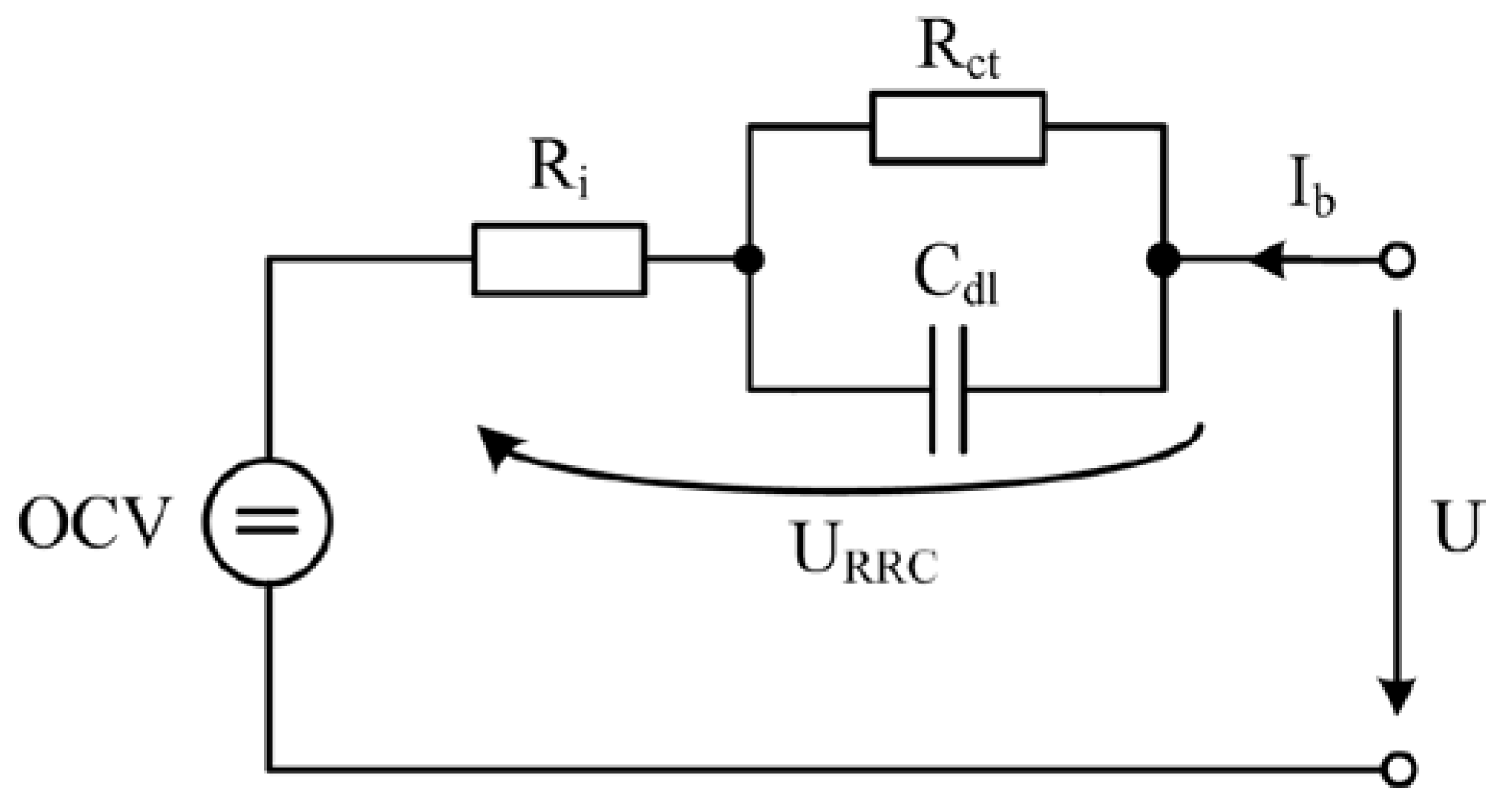
An ECM for the Li-Ion battery is shown in
Figure 1. The terminal voltage (
U) of the battery constitutes an open circuit voltage (OCV) and the cell dynamic voltage fraction (
URRC) across the impedance model. The battery impedance contains an ohmic internal resistance (
Ri) connected in series with an
R–C parallel circuit, composed of a charge transfer resistance (
Rtc) and a double layer capacitance (
Cdl). The electrical behavior of the ECM in the s-domain can be expressed as Equation (1).
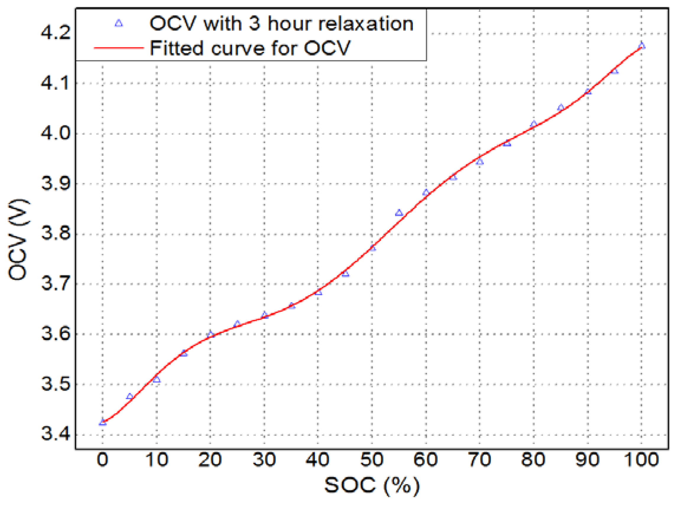
The OCV–SOC relationship, shown in
Figure 2, was modeled by a seventh order polynomial function of SOC, as described by Equation (2).
The dynamic voltage fraction of the battery (
UHPF) and the battery current (
IHPF) were extracted using high-pass filtering of the measured terminal voltage and current of the cell, respectively. The dynamic voltage (
UHPF), which is the voltage drop across the
Ri and
Rct–Cdl network, can be expressed as:
The transfer function G(s) can be obtained from Equation (4).
The forward Euler transformation method, shown in Equation (5), was employed to discretize the transfer function. Thus, the discrete transfer function of the battery model with sampling time
T can be obtained using Equation (6).
where
z is the discretization operator.
where
Following discretization, the relationship between various samples of input and output can be expressed by Equation (8), by rewriting Equation (3) in the discrete time domain.
Equation (8) is the specific form of the ARX model given in Equation (9), for the ECM shown in
Figure 1 [
19].
In terms of online parameter estimation, the terminal voltage and current were sampled at a specific constant time period, and then, the model parameters were estimated using an RLS algorithm, as explained in
Section 3.
3. Online Parameter Identification Algorithm
A recursive least square algorithm was used to estimate the coefficient factors,
a1,
b0, and
b1 [
20]. To identify the model parameters, the ARX form in Equation (9) was rewritten in the form of a recursive function.
where
Here, φk is the input data matrix obtained from the input data, consisting of the high-pass filtered voltage (UHPF) and current (IHPF) of the battery at time indexes k and k − 1. θk is the parameter matrix containing the coefficients to be identified.
The gain, , of the RLS algorithm is shown in Equation (13).
The estimated coefficient vector, , can be represented by Equation (14).
The covariance matrix,
, of the estimated coefficient vector,
, is shown in Equation (15).
where the forgetting factor,
λk, is typically set to a value between 0.95 and 1, which can be used to give more weight to recent data when compared with old data [
20].
After identifying
a1,
b0, and
b1, the parameters of the battery model at each time step can be determined using an inverse parameter transformation, as shown in Equation (16).
4. SOC Estimation Using a Nonlinear State Observer
A battery system is highly nonlinear, as observed in the SOC–OCV relationship given in Equation (2). Therefore, a nonlinear state observer (NSO) was used for SOC estimation of the lithium-ion battery. Based on the battery model shown in
Figure 1, the state space equation of the battery was formulated as shown in Equation (17).
where
UCdl is the voltage drop on the double layer capacitance (
Cdl),
η is the Coulomb efficiency of the cell,
Ib is the battery current, and
Cn is the nominal capacity of the battery.
The observation equation of the battery can be expressed as Equations (18) and (19).
The instantaneous OCV was calculated based on the nonlinear OCV–SOC function given in Equation (2), and the dynamic voltage fraction was reconstructed by extracting the impedance values using Equation (16). Finally, the estimated terminal voltage of the battery was established in the form of an observation equation, as shown in Equation (20).
where the “^” operator over the letter
U indicates estimated values. The Lyapunov stability theory was used to verify the convergence of the NSO [
20].
The eigenvalue, ζ, of matrix A was calculated, and the results are shown in Equation (21).
Therefore, the nonlinear observer can be represented as Equation (22), where a difference between the estimated voltage,
, and the measured voltage of the battery,
U, leads to an update of the battery state, as shown in Equation (22).
where the gain
K is a symmetric matrix and a positive definite solution to the Lyapunov function shown in Equation (23).
where the rank of matrix
D is equal to that of
A. Both matrix
K and its inversion
K−1 are positive definite, and
d,
k1, and
k2 are undetermined positive constants.
The observer error can be expressed by Equation (25).
The following result states that the observer error is asymptotically stable by using the Lyapunov function, which was selected as shown in Equation (27) [
20].
Its derivative was selected as shown in Equation (28).
where
Then, M can be proven to be a positive definite matrix using a non-zero column vector, , as described in Equation (30). Where a and b are real numbers,
Thus, is a negative definite, and as a result the error system in Equation (25), is asymptotically stable. Each dynamic system in Equations (20) and (22) can be selected as an observer for the system in Equations (18) and (17), respectively.
The NSO in Equation (22) enables online SOC estimation of the battery by evaluating the sequences of measured battery voltage and current through the information of the battery parameters.
5. SOC Estimation of Multiple Cells in a Battery Module
The computational burden of the SOC estimation algorithm, as discussed in
Section 4, is quite heavy when applied to multiple batteries. In order to reduce the calculation efforts of SOC estimation for multiple cells, a simplified cell model was used in combination with a lean algorithm based on vector computation, so as to enable access to the SOC of individual cells. In this method, the SOC of individual cells was estimated by evaluating the OCV, as well as the gradient of the OCV–SOC curve at an instantaneous operating point. The calculations were performed using Equations (31) to (40) [
21].
The dynamic voltage of each cell of the battery module forms the vector Uc as shown below.
The mean cell voltage, , was derived by taking an average value of the vector Uc elements as shown in Equation (32).
Under certain current excitations, the voltage drops across cells connected in series differ depending on the actual impedance of each battery cell. A higher impedance of the cell causes a higher voltage drop across it.
Therefore, the vector of the dynamic cell voltage fractions can be expressed by Equation (33).
where vector
L reflects the ratio of each cell’s impedance, calculated by considering the dynamic voltage fraction of the cell voltages.
The deviation of Up from individual cell voltage, Uc, manipulates L as shown in Equation (34).
The derivation of SOC–OCV curves produced an OCV gradient, m, as shown in Equation (35).
The OCV variation vector, ΔOCV, of n cells can be estimated using Equation (36).
The estimated individual OCV values of cells according to the ratio vector, L, and the dynamic voltage fraction of an average cell, URRC, can be expressed by Equation (37).
The difference in OCV variation between the measurement and the model was then calculated using Equation (38).
The cell’s individual SOC variation vector, ΔSOC, can be recursively calculated by Equation (39), by considering the impedance data, where
gcell is the feedback gain.
Finally, the individual cell’s SOC value, which was calculated using Equation (40), is the sum of the cell’s SOC variation and the SOC value of the average cell.
6. Experimental Results
In order to prove the validity of the proposed algorithm to estimate the SOCs of multiple Li-ion batteries using an NSO, six battery cells connected in series were used for the experiments. The specifications of the Li-ion battery can be found in
Table 1.
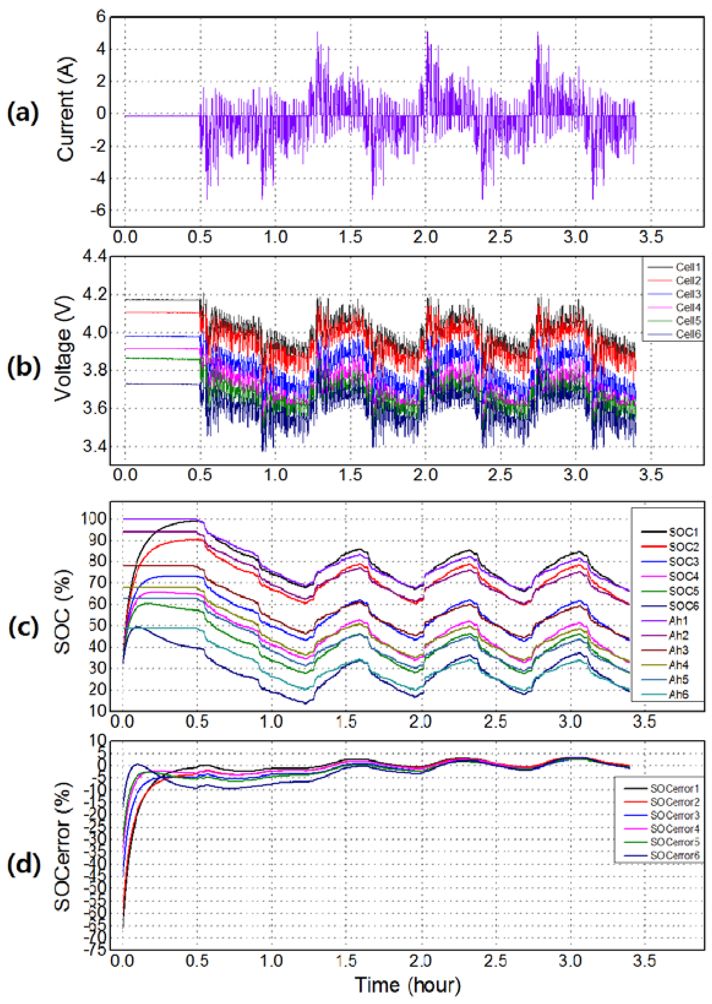
The C-rate is a measure of the rate at which a battery is charged or discharged relative to its nominal capacity. A dynamic charge/discharge current profile, as shown in
Figure 3a, was applied to the battery. A 1/20 scaled-down battery current profile was required for the electric vehicle to complete eight cycles of the Urban Dynamometer Driving Schedule (UDDS), started after a 30-min relaxation time at the beginning of the test. It can be seen in
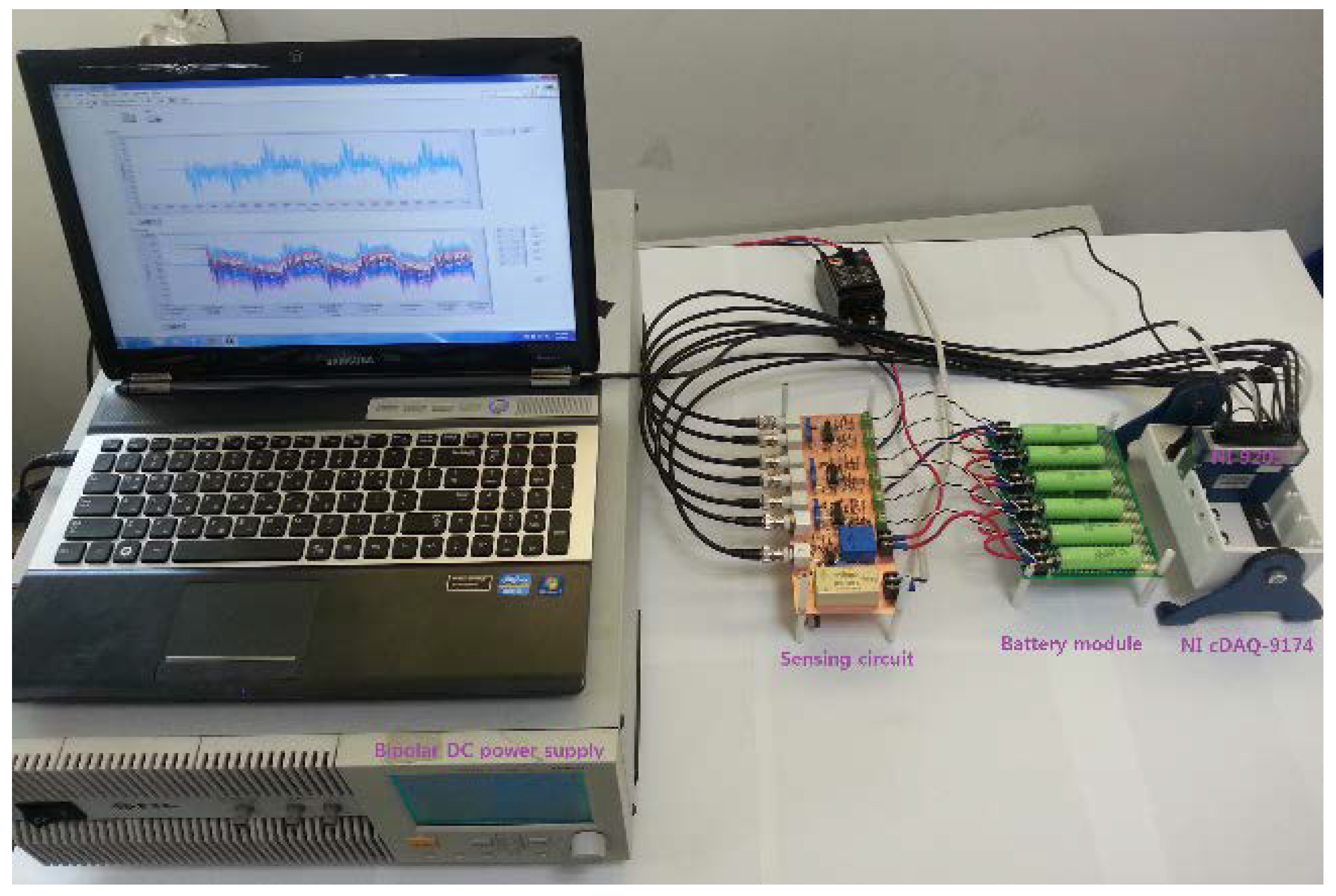
Figure 3 that each UDDS cycle lasted for 22 min, and the SOC increased or decreased by 15% at each cycle. Therefore, the direction of current in UDDS cycles numbers 3, 5, and 7 was reversed. The actual SOCs of the cells were in between 20% and 85% SOC; thus, no cell was fully discharged. The current profile was specially designed in accordance with the actual working environment of EV applications. Moreover, it exhibited dynamic characteristics with stiff changes in magnitude of the current, and operated in between high and medium SOC, which is a common operating range of SOCs in EV applications. At first, the current profile was applied to a single cell. The cell was connected to a bipolar power supply (NF BP4610). A program created in Labview 11.0 automatically controlled the output of the bipolar DC supply, and recorded the voltage and current of the battery every second through an NI PCI-9205 and a sensing circuit, which had one current sensor and six voltage sensors. The ambient temperature during the test was 25 °C.
In order to compare the performance of the proposed method, another method using a linear state observer (LSO) was implemented according to References [
21,
22], and tested for SOC estimation in the module with multiple lithium-ion batteries.
Figure 3b depicts the battery voltages estimated with the NSO and the LSO, and the measured voltage obtained from the experiments. The relative errors between them are shown in
Figure 3c as a function of time. The results show that the NSO method provided more accurate results than the LSO method in terms of voltage estimation. The average voltage estimation error of the NSO was 0.360%, which was less than that of the LSO (0.416%).
Figure 3d shows the estimated SOCs with the NSO and the LSO, and their errors with respect to the SOC calculated by the Coulomb-counting method. The battery was fully charged by constant current/constant voltage (CC-CV); thus, it was at 100% SOC prior to the test. Since the initial SOC was known, and the test occurred in a short period of time, the Coulomb-counting method could be used as a reference by neglecting error accumulation. In the experiments, 50% of the SOC was given as an initial value to verify the convergence of the proposed algorithm. As shown in
Figure 3e, the estimated SOC tracked the true SOC value within 30 min, keeping the estimation error of the NSO less than 3%, while the estimation error of the LSO exceeded 4%. The SOC estimation results using the NSO were better than those using the LSO.
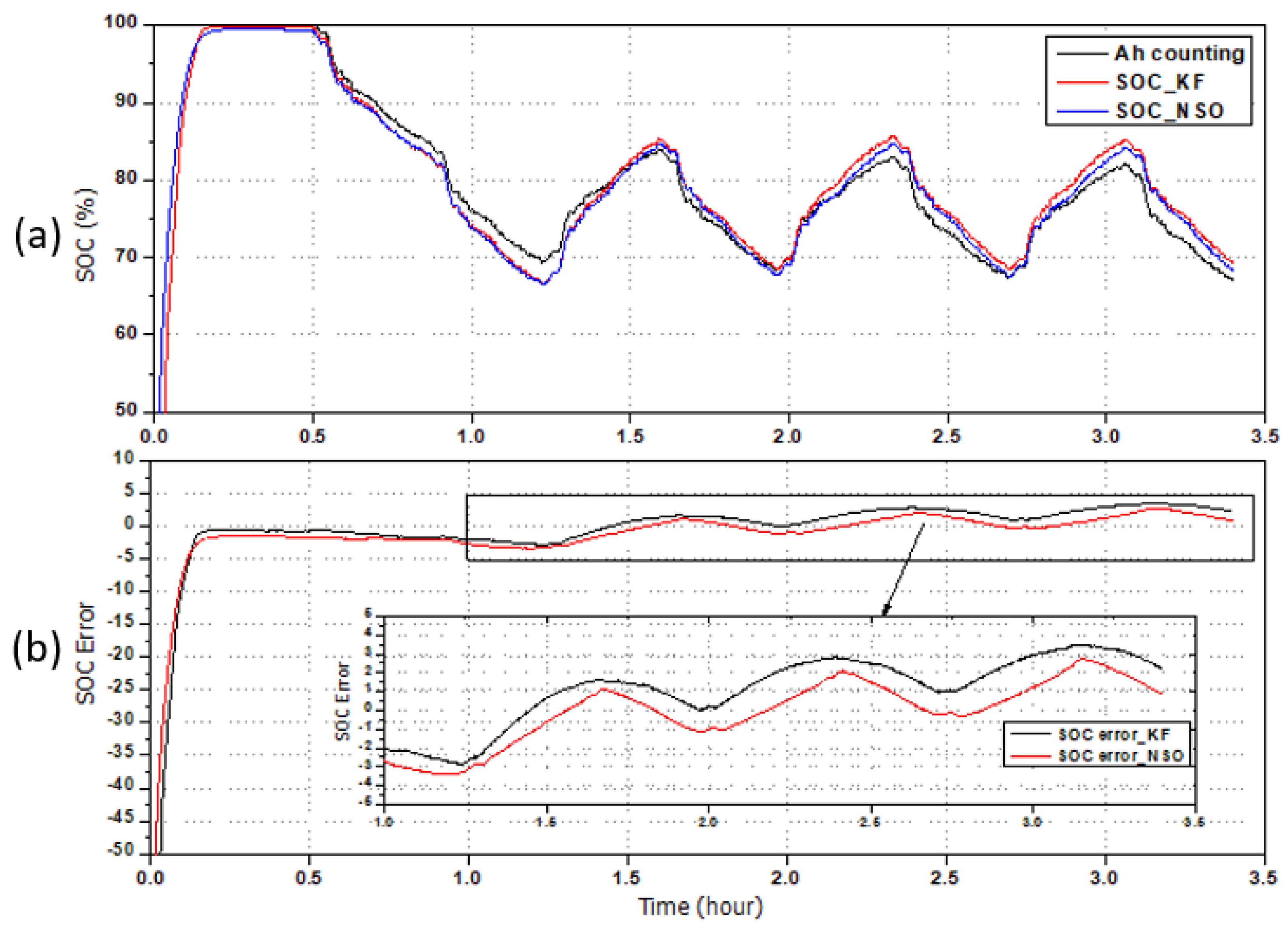
Figure 4 shows the SOC estimation results using an extended Kalman filter (EKF) [
5] and the NSO. Since SOC estimation of lithium batteries is often implemented using EKFs, it was required to compare the accuracy of SOC estimation of the proposed method to that of EKF. As shown in
Figure 4, the SOC estimation accuracy using the NSO was around 0.5% better than that using the EKF. Since SOC estimation is required for multiple cells in a module, computational burden is also a very important aspect which needs to be considered.
Figure 4 shows the SOC estimation performances using the NSO and the EKF, and the summary of the results can be found in
Table 2. As shown in
Table 2, the execution time of each method was measured by running the code with a desktop personal computer, which had a Core i7 processor and 8 GB of Random-Access Memory (RAM). It can be observed from
Table 2 that SOC estimation using the NSO was better than that using the EKF in terms of maximum error and root-mean-square error (RMSE), while the computational burden of the NSO was 62% less than that of the EKF.
In order to validate the proposed algorithm for multiple cells, the same current profile was applied to a module, consisting of six cells connected in series.
The experimental setup for the battery module test is shown in
Figure 5. The current profile is shown in
Figure 6a, and the voltage response of each cell in the battery module is shown in
Figure 6b.
Figure 6c shows the estimated SOC values of individual cells in the module using the proposed method, and using the Coulomb-counting method during the test.
The SOC estimation errors are shown as percentages in
Figure 6d. In the experiments, all initial SOC values of the cell were set to 30% to verify the convergence of the proposed algorithm.
As shown in
Figure 6d, the estimated SOC of each cell in the module tracked the true SOC after 1.5 h, and the estimation error of each cell was less than 3.5% thereafter.


