In Situ Experiment and Numerical Model Validation of a Borehole Heat Exchanger in Shallow Hard Crystalline Rock

Abstract

Accurate and fast numerical modelling of the borehole heat exchanger (BHE) is required for simulation of long-term thermal energy storage in rocks using boreholes. The goal of this study was to conduct an in situ experiment to validate the proposed numerical modelling approach. In the experiment, hot water was circulated for 21 days through a single U-tube BHE installed in an underground research tunnel located at a shallow depth in crystalline rock. The results of the simulations using the proposed model were validated against the measurements. The numerical model simulated the BHE’s behaviour accurately and compared well with two other modelling approaches from the literature. The model is capable of replicating the complex geometrical arrangement of the BHE and is considered to be more appropriate for simulations of BHE systems with complex geometries. The results of the sensitivity analysis of the proposed model have shown that low thermal conductivity, high density, and high heat capacity of rock are essential for maximising the storage efficiency of a borehole thermal energy storage system. Other characteristics of BHEs, such as a high thermal conductivity of the grout, a large radius of the pipe, and a large distance between the pipes, are also preferred for maximising efficiency.

1. Introduction

Solar thermal energy is a renewable energy source that can be used to cover space heating and domestic hot water demand in buildings. In high latitudes, solar energy is most abundant in the summer months when the space heating demand is the lowest, and less abundant in winter months when the space heating demand is the highest. The solution is to collect the thermal energy in low demand periods, store it seasonally using one of the underground thermal energy storage (UTES) methods, and use it during times of high demand. A viable option for storing the energy is the borehole thermal energy storage (BTES) method that utilises an array of borehole heat exchangers (BHE) installed in the ground, which serve as the storage medium [1].

The goal of this study was verification of the Heat Transfer in Pipes (HTiP) modelling approach of BHE that will be used to model large BTES systems. The first objective of this study was to compare the simulation with measurements from an in situ experiment of a single BHE installed in hard crystalline rock. The research question posed was, does the HTiP approach model the behaviour of the BHE accurately and what is the error? The second objective was to compare the HTiP model with two other approaches from the literature to quantify the accuracy and efficiency of the HTiP model and to evaluate if it is appropriate for the modelling of large BTES systems. The last objective was to investigate the sensitivity of the HTiP model to draw practical conclusions related to design aspects of BTES. The research question posed was, what practical conclusions can be drawn from an operation of a single BHE that would apply in seasonal storage using large BTES systems?

Precise and computationally-efficient numerical models of BHEs are needed for simulation of large BTES systems where the number of BHEs can reach more than 200. These numerical models are also required to perform well over both short and long timescales to accommodate for varying charging and discharging rates. Analytical models give the simplest and quickest solutions. A solution to a finite line heat source model was given by Ingersol and Plass [2], where the BHE was approximated as a line heat source. Carslaw and Jaeger [3] gave another solution representing a cylindrical heat source with a radial dimension added so that the BHE was represented as an infinite cylinder in a homogeneous ground. The analytical solution was implemented by Eskilson [4] into a finite difference two-dimensional model assuming steady-state conditions for heat transfer in the borehole. The model used g-functions—dimensionless coefficients used for determining the thermal performance of different BHE configurations. Hellström [5] presented a numerical model based on the analytical solution for local heat transfer with a superposition principle to calculate the added effect of multiple boreholes. However, analytical solutions require simple geometries and do not consider the transient heat transfer, which means they are not suitable for short-term simulations.

More sophisticated analysis can be done using numerical models. The thermal performance of a BHE can be simplified to a 1D problem using linear elements and a thermal resistance network. A numerical solution using a finite element method was first proposed by Al-Khoury et al. [6,7]. The method was later improved by modification of the thermal resistance network and the introduction of thermal resistance and capacity models [8]; the method has been implemented in finite element code [9,10]. The method allows the calculation of transient heat transfer in single and double U-tubes and two coaxial types of BHE. An example where this approach was used to model a large BTES system was presented in [11]. Further improvement was made by dividing the grout into three zones with the aim of increasing the accuracy of the spatial representation of the system [12,13].

Other simplified numerical approaches were presented by Ozudogru et al. [14] and Holzbecher and Rauschel [15] with the U-tube pipes being also represented as 1D elements, but with a slightly modified approach. The former introduced the so-called pseudo-pipes to overcome the absence in the pipe’s heat capacity, and the latter presented a method to discretise the pipes using the extruded linear element to simplify the geometry and limit the number of elements.

The most sophisticated numerical approach is based on a three-dimensional model with fully-discretised BHE and coupled flow and heat transfer inside the pipes and in the ground (e.g., the finite volume model in [16]). The main advantage of this approach is that the thermal behaviour of the BHE can be simulated over very short timescales, so that the dynamic variations of the heat transfer are not omitted. An efficient method with fully discretised BHE was presented by Oberdorfer et al. [17,18] and by Oberdorfer [19]. The model assumed a mean fluid velocity that represented a fully-developed flow inside the pipes, and the effective thermal conductivity was calculated based on the average flow velocity and constant parameters. This resulted in a reduction in calculation speed, but the model was precise enough to simulate the BHE’s behaviour on both short and long timescales.

In this study, simulation of the heat transfer inside the BHE was accomplished by the use of the Heat Transfer in Pipes (HTiP) modelling approach, which uses an existing HTiP physics interface in the pipe flow module in the COMSOL Multiphysics 5.3a finite element software package [20]. The interface allows for a 1D simulation of fluid flow and heat transfer in pipe networks. It is coupled with a 3D heat transfer in the surrounding solid to simulate the heat transfer through the heat exchanger pipe wall into the surrounding grout. The HTiP approach combines the advantages of other numerical methods identified in the literature analysis, because the heat transfer inside the heat exchanger pipes is simplified to one dimension, similar to refs. [6,7,8,9,10,11,12,13], which reduces the number of finite elements needed, therefore reducing the calculation speed. However, only the pipes of the BHE are reduced to 1D, and the grout is kept as a 3D object in the same way as in refs. [15,17,18,19], which allows modelling of more complicated BHE geometrical arrangements. Furthermore, the simulation can be done on both short and long timescales, similarly to refs. [16,17,18,19]. The use of the HTiP model for thermal simulation of subsurface heat exchanger systems has been demonstrated in refs. [14,21,22]. Previous authors have used the HTiP model for numerical prediction of an in situ experiment [23].

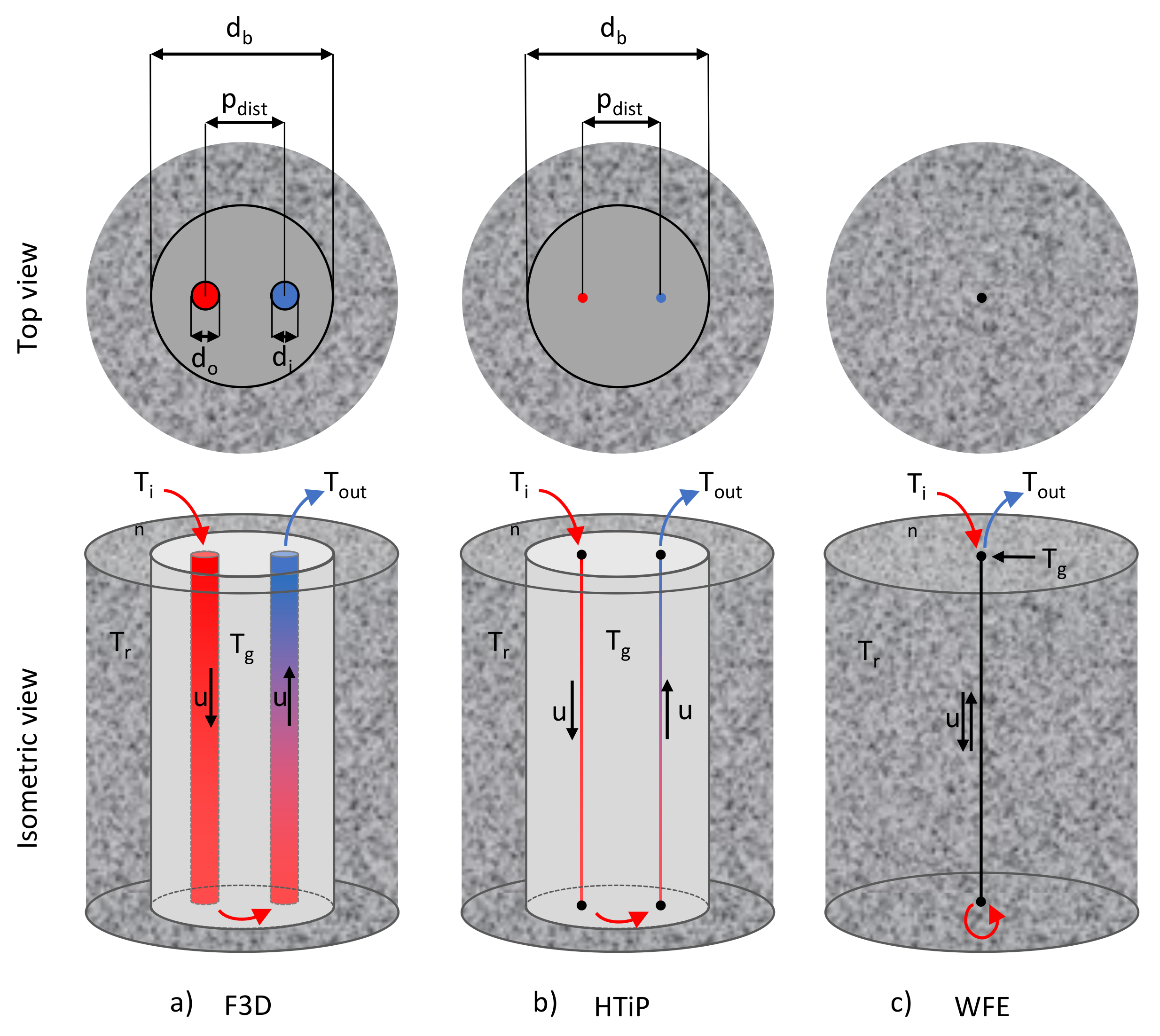
Based on the literature analysis, two methodologies were selected to study the effect of the reduction in dimensions of BHE geometry on the precision and computational effort of the heat transfer analysis inside the BHE; these methodologies were compared with HTiP. The first modelling approach used for comparison was a method described in [17], in which the BHE is modelled as a three-dimensional object with the explicit geometry of the pipes and the surrounding grout (F3D, see Figure 1a). The heat transfer through the pipes is calculated based on an effective thermal conductivity of the pipes, which depends on the mean fluid velocity [17]. Due to the explicit representation of the BHE, this approach has a lower level of dimension reduction of the BHE geometry and requires more finite elements in the model compared to HTiP. Hence, the expected computational requirements are higher. However, the F3D model is expected to be more precise, because it circumvents the estimation errors in the HTiP methodology related to (i) the coupling of the pipe wall temperature at the pipe axis instead of at the correct location at the outer pipe radius, and (ii) not accounting for the heat capacity of the pipes.

The second modelling approach used for comparison was a more simplified method that uses weak form equations (WFE) to simulate the thermal performance of a BHE [6,7]. The BHE is represented as a one-dimensional edge that is embedded into a three-dimensional medium, and the level of dimension reduction of the BHE is higher compared to HTiP (Figure 1c). The solution regarding the heat transfer inside the BHE is approximated using the weak form equations, which are coupled to the heat transfer in the rock mass through shared node points on the BHE’s linear edge. A detailed description of this modelling approach can be found in refs. [6,7,24]. This approach is much faster compared to HTiP and F3D as it requires much fewer finite elements. However, it is not as accurate due to simplification and parametrisation of the BHE geometry.

2. HTiP Numerical Modelling Approach

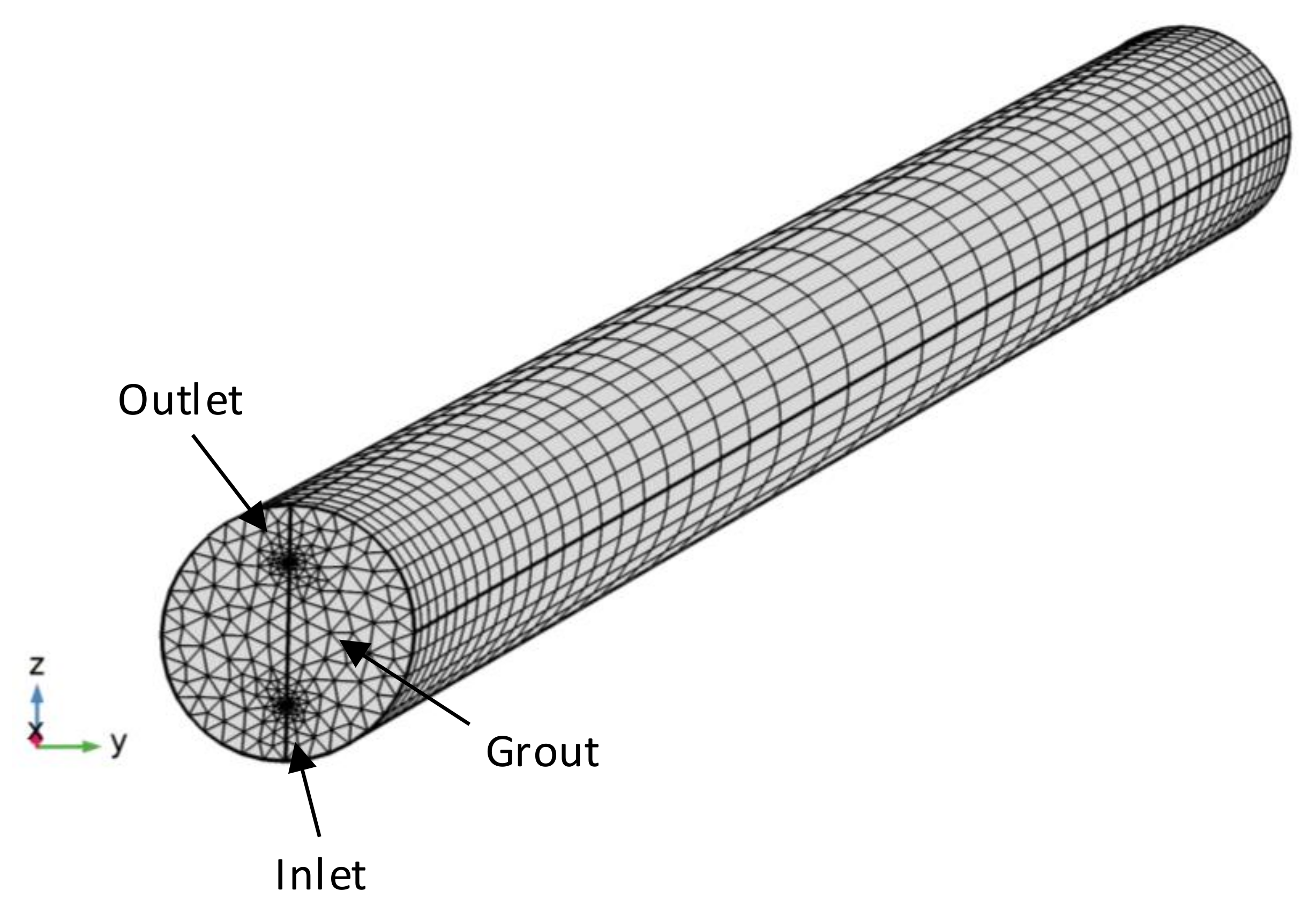
In the HTiP approach, the pipe-in and pipe-out of the single U-tube BHE are modelled as one-dimensional lines embedded into a three-dimensional grout domain (see Figure 1b). Since the pipe cross-sections are not discretised, computation time is reduced and the memory requirement is lower. The heat transfer inside the pipes (see Equation (1)) is based on the average velocity of the fluid with an assumption that the flow is fully developed. The heat transfer inside the pipes is described via a one-dimensional energy equation for incompressible fluid which is based on convection–diffusion equation with additional contributions [20,25]:

$${\rho }_f{A}_p{C}_f\frac{\partial T_f}{\partial t}+{\rho }_f{A}_p{C}_{f}u·\nabla T_f=\nabla ·A_p{\lambda }_f\nabla T_f+f_D\frac{\rho A_p}{2d_h}{\left|u\right|}^3+Q_{wall},$$

(1)

where $T_f$ is the dependent variable of fluid temperature (K), ${\rho }_f$ is the fluid density (kg/m³), $C_f$ is the fluid heat capacity at a constant pressure (J/(kg∙K)), ${\lambda }_f$ is the fluid thermal conductivity (W/(m∙K)), and $u$ is the tangential average fluid velocity (m/s). The $A_p$ is the area of the inner pipe, $d_h$ is the hydraulic diameter of the pipe equal to the inner diameter for a pipe of circular shape. The $f_D$ is the Darcy friction factor due to flow resistance, which describes the continuous pressure drop along the pipe wall due to viscous shear and is calculated in accordance with the Churchill friction model [26].

The source term $Q_{wall}$ in Equation (1) is the radial heat transfer across the pipe wall (W/m), which is governed by the temperature difference between the grout and the fluid. It provides coupling from the surrounding 3D grout temperature to the fluid temperature (see Equation (3)) and is calculated with [20].

$$Q_{wall}={\left(hZ\right)}_{eff}\left(T_{grout}-T_f\right),$$

(2)

where ${\left(hZ\right)}_{eff}$ is the effective heat transfer coefficient, computed according to ref. [20]. The effect of a boundary layer inside the pipes is taken into account in the form of the internal film heat transfer coefficient. In this study, only internal turbulent forced convection was expected ($Re$ > 3000), hence the Gnielinski Equation [27] was used for calculations of the Nusselt number.

The transient heat conduction in the rock and grout was calculated using the following Equation [20]:

$$\rho c\frac{\partial T}{\partial t}+\nabla ·\left(-\lambda \nabla T\right)=Q_{wall}$$

(3)

where $T$ is the dependent variable of temperature (K), $\rho$ is the density (kg/m³), $c$ is the heat capacity (J/(kg∙K)), and $\lambda$ is the thermal conductivity (W/(m∙K)) of the rock and grout. The $Q_{wall}$ is the source term representing the heat transfer from the fluid to the grout, which couples Equations (1) and (3).

3. In Situ Experiment for Numerical Model Verification

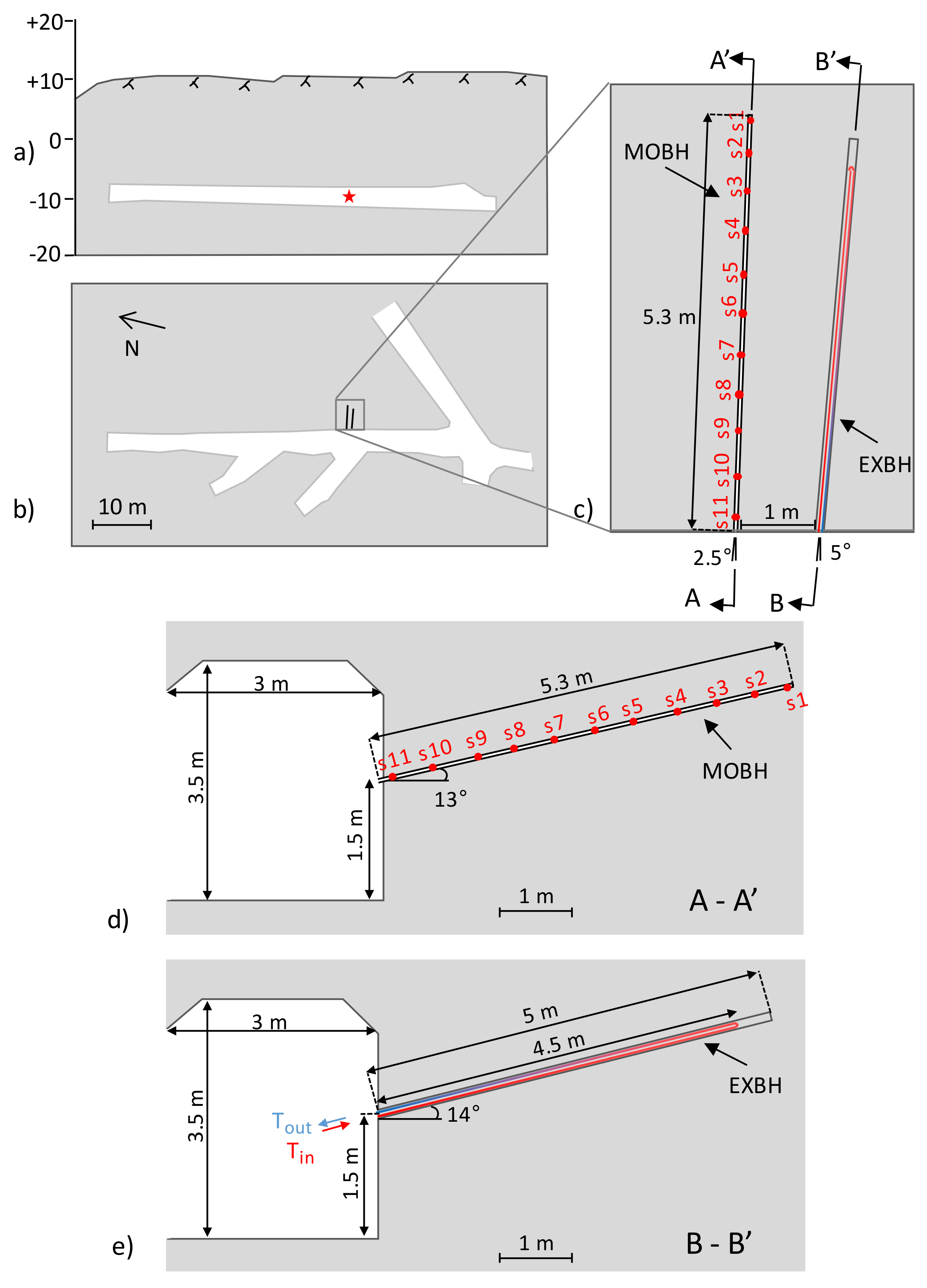
The in situ experiment was designed to verify the proposed numerical modelling approach of a single BHE. The experiment was conducted in 2017 in the research tunnel of Aalto University situated under the Otaniemi campus in the city of Espoo, Southern Finland. A comprehensive description of the in situ experiment can be found in ref. [28]. The research tunnel under Otaniemi Campus (Figure 2a,b) has a length of 60 m from the entrance to the back wall. The tunnel is horseshoe-shaped with straight walls and an arched ceiling. The roof is supported with rock bolts, and a 3 cm sprayed concrete layer is used to reinforce both roof and walls.

The depth from the surface to the tunnel roof is approximately 20 m, varying by the position along the tunnel (Figure 2a). The location selected to drill the experiment borehole is located at 19 m from the entrance. In this area, the width and height of the cross-section are 3 m and 3.5 m, respectively.

Finland is located on an old and stable bedrock that is part of Fennoscandian Shield of the Archaean (3100–2500 Ma) and Proterozoic (2500–1300 Ma) eras. The bedrock is composed of granitoids and gneisses. Other metavolcanic or metasedimentary lithologies are also present [29]. It is covered by Quaternary soil layers that are less than 5 m thick, on average, due to the advancement and melting of glaciers during the last Ice Age. The rock mass around the tunnel is composed of two main rock types: fine-grained hornblende–biotite gneiss and migmatic granite, which are typical rocks found in Southern Finland.

The experiment configuration consisted of two inclined, nearly-parallel boreholes drilled into the wall of the tunnel. The experimental borehole (EXBH) was drilled with a 107 mm diameter, at a height of 1.5 m above the tunnel floor, at an angle of 14° from the horizontal plane and 5° from the vertical plane (see Figure 2e). The monitoring borehole (MOBH) was drilled with a diameter of 47 mm, at a height of 1.5 m above the tunnel floor, at an angle of 13° from the horizontal plane and 2.5° from the vertical plane (see Figure 2d). The drilling was performed with a handheld drill.

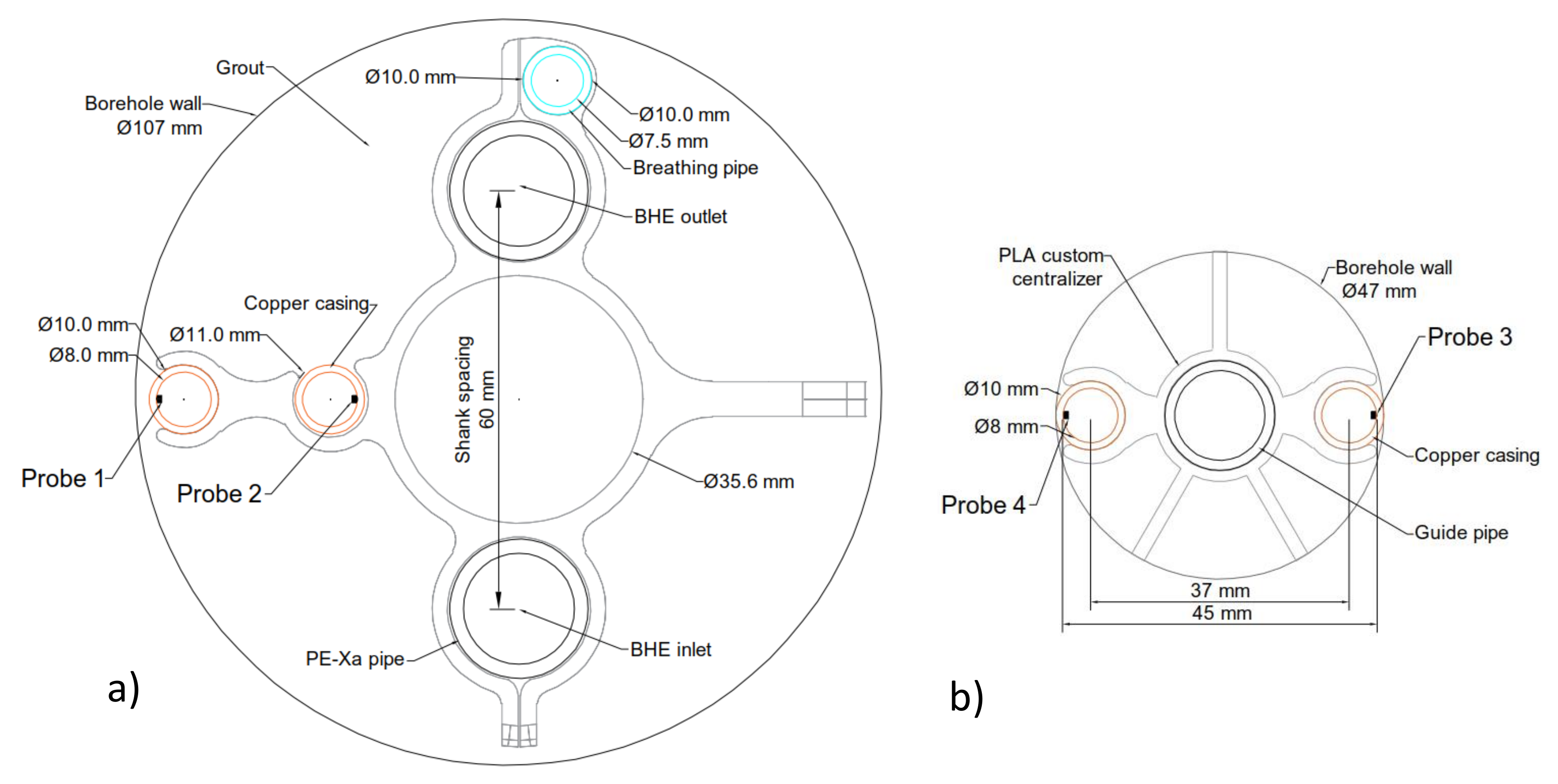
A single U-tube BHE was installed in the EXBH (Figure 3a). The BHE was composed of two PEX-a pipes connected by a brass U-turn. The pipes were grouted in place using pure sulphate-resistant cement, Plussementti CEM II/B-M (S-LL) 42,5 N, mixed with water. A breathing pipe was used to allow for the removal of air from the grout. Samples of the grout material were collected at the start and end of the grouting process to assess the quality of the final product. The density of the grout samples was equal to 1925.7 kg/m³, on average. Customized pipe centralisers were used to keep the pipes in the borehole at the correct shank spacing of 60 mm (see Figure 3a).

The BHE was connected to a 3 kW water heater with 15 L capacity and a circulation pump located before the water heater. The water heater was connected to a power regulator to regulate the power supplied to the heater to keep the circulating fluid’s temperature constant.

The experiment consisted of two phases and was continued for a total of 36 days. In the first phase, water, at approximately 57 °C, was injected into the BHE for 21 days. In the second phase of the experiment, the water circulation was stopped, and the rock mass was allowed to cool down for 15 days. In this study, only the heating phase was taken into account as it is directly related to the performance of the BHE.

The thermal conductivity and thermal diffusivity of the rock were measured in the laboratory using an optical thermal conductivity scanner (TCS). Six samples representing the two rock types were extracted from the tunnel walls. The average thermal conductivity obtained in the TCS test was 2.77 W/(m∙K) for gneiss and 2.97 W/(m∙K) for granite. The average thermal conductivity of the two rocks was 2.87 W/(m∙K), and the thermal diffusivity was 1.51 × 10⁻⁶ m²/s. An average thermal capacity of 723.5 J/(kg∙K) was calculated from the values obtained from the TCS and density measurements. The resulting values are in line with the average thermal properties of Finnish rocks, as reported by Kukkonen and Peltoniemi [30].

Two main fractures were found in the boreholes using a borehole video camera, but no groundwater inflow was identified. In the EXBH, a vertical fracture was found to traverse the borehole between the 2.5 and 3.2 m borehole depths. A small cavity in the vicinity of the fracture was identified that formed, most probably, as a result of borehole reaming, as rock flakes were retrieved during the reaming process. In the MOBH, a smaller fracture was found around the 2.0 m depth mark. The fracture’s aperture was not measured. However, it is highly likely that if the fractures were open, they were filled with grout as no significant differences in rock temperature along the MOBH could be measured at that depth. Additionally, a thermal response test was performed in the investigated borehole. The predicted effective thermal conductivity of the borehole configuration was found to be equal to 2.86 W/(m∙K), which is almost identical to the values found in the laboratory test of the rocks samples from the tunnel. The investigation of the fractures on the tunnel surface was not done due to a presence of shotcrete layers that cover the tunnel walls and the roof.

The rock temperature in the MOBH was measured in real-time by customised equipment built for the project. There were two sets, consisting of eleven DS18B20 digital thermal sensors each (see Figure 2c,d, sensors s1 to s11), that were installed on opposing walls of the monitoring borehole (see Figure 3b). The set of sensors installed on the borehole wall closest to the heat source is referred to as Probe 3 and the opposite set of sensors as Probe 4. The sensors were inserted into 4 cm long copper tubes to provide good contact with the borehole wall. The sensors were fixed inside the MOBH by customised centralisers (see Figure 3b). Unfortunately, the connection with all temperature sensors installed in the EXBH (Probe 1 and 2 in Figure 3a) was lost during the grouting process and no data could be retrieved.

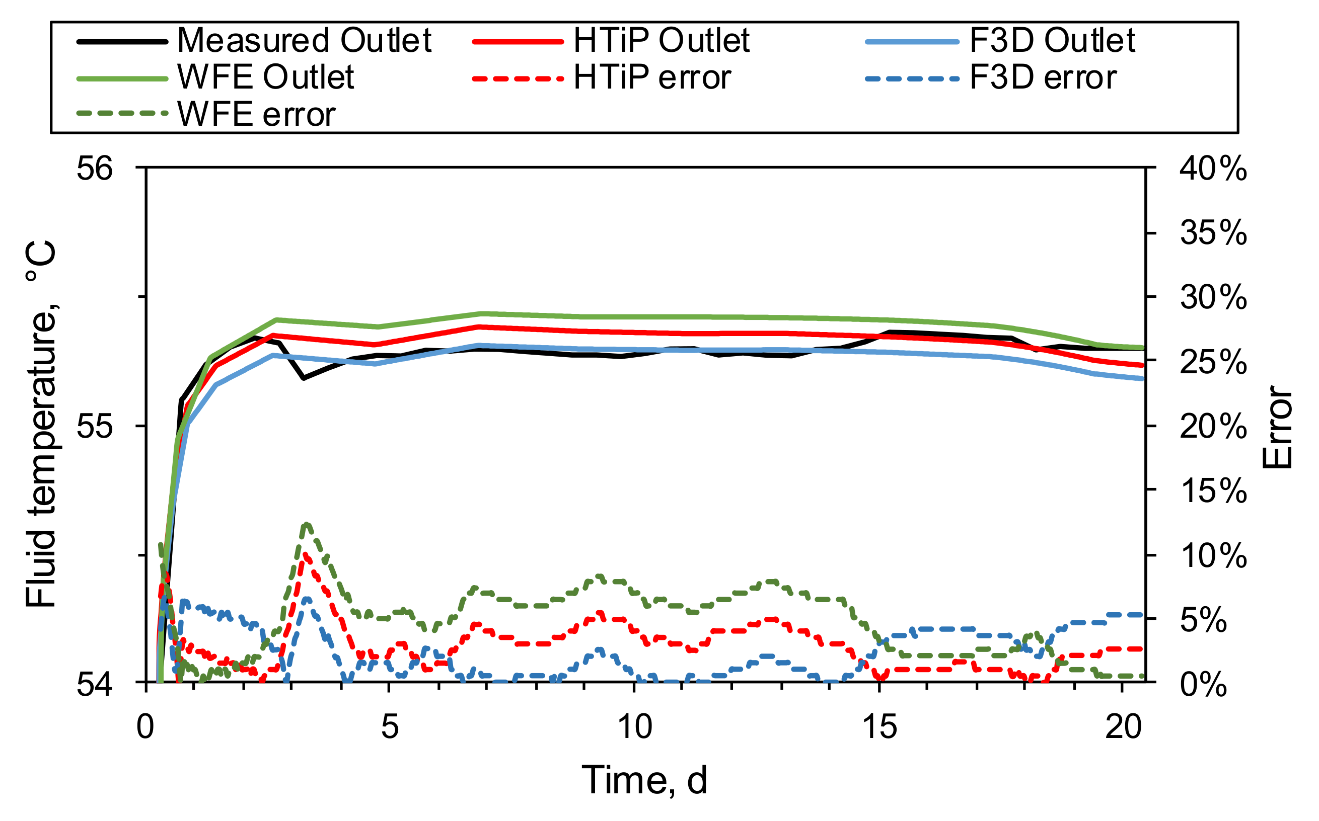
The heat carrier fluid used in the experiment was tap water. The temperature of the fluid was monitored by two flow-through thermal sensors installed in the BHE’s inlet and outlet. A power controller was used to regulate the input temperature at a constant level of 57.3 °C over the 21-day period, as seen in Figure 4. The outlet temperature was nearly constant during the 21-day period with an average value of 55.3 °C.

A flow meter measured the flow rate of the carrier fluid in the system with a pulse counter, factory calibrated to one litre per second for every 77 pulses. The goal was to fix the velocity of the fluid at a constant level. However, the flow velocity was not constant, but slowly decreased from 0.4 to 0.35 m/s, as seen in Figure 4.

4. Numerical Simulation of the In Situ Experiment

A 3D numerical model of the in situ experiment was built using the COMSOL Multiphysics 5.3a software package [20], which is based on the finite element method. The goal of the modelling was a validation of the HTiP modelling approach and a comparison with the WFE and F3D modelling approaches. The resulting fluid temperature at the BHE outlet and the rock temperatures at sensor locations in the monitoring borehole given by all three approaches were compared with the measurements obtained in the experiment. Both the absolute values and the relative error of the simulated and measured temperatures were compared. The relative error of the simulated fluid temperature drop was calculated by taking the absolute difference between the measured and simulated temperature drop (the difference between inlet and outlet) and diving it by the measured temperature drop:

$${\epsilon }_{\Delta T_{fluid}}=\frac{\left|{(T_{outlet}-T_{inlet})}_{sim}-{(T_{outlet}-T_{inlet})}_{meas}\right|}{\left|{(T_{outlet}-T_{inlet})}_{meas}\right|}\times 100\%$$

(4)

The same methodology was used to compare the deviation between the measured and simulated temperature increase of the surrounding rock after the heating phase:

$${\epsilon }_{\Delta T_{rock}}=\frac{\left|{(T_{end}-T_{start})}_{sim}-{(T_{end}-T_{start})}_{meas}\right|}{\left|{(T_{end}-T_{start})}_{meas}\right|}\times 100\%$$

(5)

4.1. Numerical Model Set-Up

The model of the experiment consisted of a cuboid representing the rock mass with a height, width, and depth equal to 48.7 m, 86 m and 71.2 m, respectively (see Figure 5). The dimensions were selected based on calculations of the travelling time of the thermal front to ensure that there was no influence of the outer surface temperature boundary condition on the results. The upper surface of the rock mass was located at +10.9 m and represented the ground surface.

Two rectangular tunnels were included in the model, representing a simplified tunnel network in the vicinity of the experiment site (see Figure 5). The experiment took place in Tunnel A, and its dimensions are given in Figure 2d. To simulate the effect of the tunnel’s air temperature on the temperature of the rock mass, Tunnel B was included in the simulation (see more details in the section on pre-heating steps). The angle between the tunnels was equal to 56°. Additionally, tunnel B dipped upwards at an angle of 7°.

The geometry of the BHE differed for each modelling approach and was built according to the methodology described in the first section and visualised in Figure 1. In the HTiP model, the BHE was discretised as 3D grout and 1D pipes embedded into it. In the F3D model, the BHE was fully discretised with 3D pipes embedded into a 3D grout domain. In the WFE model, the whole BHE was simplified into a single 1D linear edge embedded into the rock mass.

The model was composed of three material domains: rock, grout, and water. The properties of the rock and the grout material are given in

Table 1. Input parameters for the numerical models of the in situ experiment.

Parameter		Value	Unit	Source
Rock thermal conductivity	λr	2.87	W/(m·K)	TCS lab test
Rock density	ρr	2504.3	kg/m3	Calculated
Rock heat capacity	cr	723.5	J/(kg·K)	TCS lab test
Grout thermal conductivity	λg	1.7	W/(m·K)	[31]
Grout density	ρg	1925.7	kg/m3	Lab test
Grout heat capacity	cg	750	J/(kg·K)	[23]
Pipe thermal conductivity	λp	0.4	W/(m·K)	[32]
Air temperature in the tunnel	Ttunnel	15.7	°C	Measured in situ
Convection coefficient at tunnel walls	h	9.9	W/(m2·K)	Iterative
Distance between pipes	pdist	4	cm	Measured in situ
Pipe inner diameter	di	16	mm	Measured in situ
Pipe outer diameter	do	20	mm	Measured in situ
Pipe surface roughness	e	0.0015	mm	[20]
Borehole diameter	db	107	mm	Measured in situ
EXBH length	exbhL	5	m	Measured in situ
MOBH length	mobhL	5.3	m	Measured in situ
BHE length	bheL	4.5	m	Measured in situ
Tunnel height	Th	3.1	m	Measured in situ
Tunnel width	Tw	2.7	m	Measured in situ
Tunnel length	TL	30	m	Measured in situ
Annual mean air temperature	TA	5.8	°C	[33]
Mean ground surface temperature	GST	7.05	°C	[34]
Geothermal gradient	dT	0.0112	K/m	[29]

. The properties of water were temperature-dependent and were imported from the software’s integrated material database.

The top surface of the model was set to an average ground surface temperature (GST), calculated based on the outside air temperature according to a relationship given in ref. [34] to account for the differences in ground and air temperatures due to snow cover: $\mathrm{GST}=\left(0.71·\mathrm{SAT}+2.93\right)$, where SAT is the mean surface air temperature.

The outer and bottom surfaces of the model were set to a constant temperature calculated as a function of the GST, increasing with depth due to the geothermal gradient which is equal to 0.0112 (K/m).

The warmer outside air temperature had steadily increased the rock temperature around the tunnels over the years. Therefore, a steady-state step for pre-heating of the rock mass was used to achieve the same initial conditions to for allow realistic temperature distribution in the rock mass surrounding the tunnel at the time (t₀) of the experiment. In the pre-heating step, a heat convection boundary condition was prescribed at the tunnels’ surfaces. To arrive at the initial rock temperature measured in the monitoring borehole, the value of the convection coefficient was iteratively found to be equal to 9.9 W/(m²·K). The coefficient approximated the exchange of temperature between the rock and the tunnel air due to air movement caused by the ventilation system installed in the tunnels. Additionally, the air temperature was set to 15.7 °C, which represents the average temperature measured in the tunnel prior to and during the experiment.

The temperature boundary condition at the BHE inlet was set according to the fluid temperature measured during the experiment and averaged per hour to even out small perturbations in the measured values that could cause a slow convergence of the solution (see Figure 4). The same methodology was used for the fluid velocity inside the pipes. The outlet fluid temperature of the pipe-in was set as the inlet temperature for the pipe-out to simulate the U-turn of the BHE at the bottom of the borehole. A heat outflow condition was prescribed at the outflow points of the pipe-in and pipe-out. It was assumed that the heat transfer over the pipe outlet boundary was convection-dominated [20].

To solve the model, a fully coupled approach was used with the MUltifrontal Massively Parallel sparse direct Solver (MUMPS) [20]. The time step was set to one hour.

The finite element mesh of the numerical model has been optimised to minimise the computational time. A commonly used technique is to build a swept mesh consisting of prisms for the meshing of the BHE domain [13,14,17]. This allows the geometry of the cross-section to be represented accurately. First, the top surface of the BHE, parallel to the tunnel’s surface was meshed with triangular mesh elements. Next, the triangular elements were swept along the borehole axis, creating prisms (see Figure 6).

A mesh sensitivity study is required to find the degree of mesh convergence so that global or local mesh refinement does not change results significantly, (i.e., the discretisation error is minimised) [35]. The mesh was optimised so that it accomplished mesh convergence but was not finer than required so that the computational expense is kept as low as possible. The number of elements was increased and the outlet fluid temperature was measured after 21 days of heating. The results of the mesh sensitivity for each modelling approach are presented in Figure 7. It can be seen that by increasing the number of elements, the fluid temperature at the outlet also increased until reaching a stable point; this was the optimal mesh size and was selected for further analysis.

4.2. Further Investigations Using the HTiP Model

A parametric study was executed to identify the most sensitive parameters in the HTiP numerical model. The parameters given in

Table 2. The range of the input parameters for the parametric study of the HTiP model.

Parameter	Range	Unit
Pipe inner radius *	2–14	mm
Grout thermal conductivity	0.25–2.5	W/(m·K)
Rock heat capacity	650–875	J/(kg·K)
Rock density	2000–2900	kg/m3
Rock thermal conductivity	2–4.25	W/(m·K)
Borehole radius	40–100	mm
Distance between pipes	0.5–5	cm
Pipe thermal conductivity	0.10–0.55	W/(m·K)

* Wall thickness kept at 2 mm.

were varied, one variable at a time, by ±25% to find the parameter that was the most influential on the result. The temperature of the fluid at the outlet and the rock temperature change at the monitoring borehole were used for the comparison of the influence of each parameter on the result.

Then, the fluid temperature at the outlet and the temperature change at MOBH were calculated as a function of changes in the input parameters by ten points within a realistic range of values (given in Table 2).

Additionally, a complete storage cycle was studied by adding a discharging phase of 21 days, wherein a constant injection of fluid into the BHE at a temperature of 10 °C was modelled numerically using the HTiP model. The goal was to simulate the discharge of the rock’s thermal storage and to calculate the storage efficiency by comparing the amount of energy discharged from the storage to the amount of energy that was charged into the rock during the 21 days of charging. The amount of energy was calculated based on the temperature difference between the inlet and outlet of the BHE. The parameters given in Table 2 were varied by one variable at a time, again by ±25%, to determine which parameters had the most influence on the storage performance of the single BHE.

5. Results and Discussion

5.1. Comparison between Measured and Simulated Results

The result of the comparison between outlet fluid temperatures measured in the experiment and simulated approaches using the HTiP and other models is presented in Figure 8. It can be seen that all three models predicted the outlet temperature fairly well. The maximum error of fluid temperature drop for the HTiP model was calculated according to Equation (4) and was found to be equal to 8.5% at the beginning of the BHE operation. The maximum error between the measured and simulated outlet temperatures was most probably caused by a rapid and short change of fluid velocity in the experiment, which was averaged out in the simulation input and was not taken into account in the model. Such a change in fluid velocity would produce a more significant temperature drop in the BHE and would result in a higher error in the simulations. Later, the error dropped and oscillated between 0% and 5%. The average error for th whole operational period of 21 days was equal to 2.9%, 2.4%, and 4.7% for the HTiP, F3D, and WFE models, respectively, which was expected due to the different degrees of dimension reduction in BHE geometry in the models (depicted in Figure 1). The F3D had the lowest level of BHE geometry dimension reduction and was found to be the most accurate. On the other hand, the WFE had the highest level of dimension reduction and produced the least accurate results. The HTiP had only a slightly higher level of dimension reduction compared to F3D, and correspondingly, the result was only 0.5% less accurate, on average.

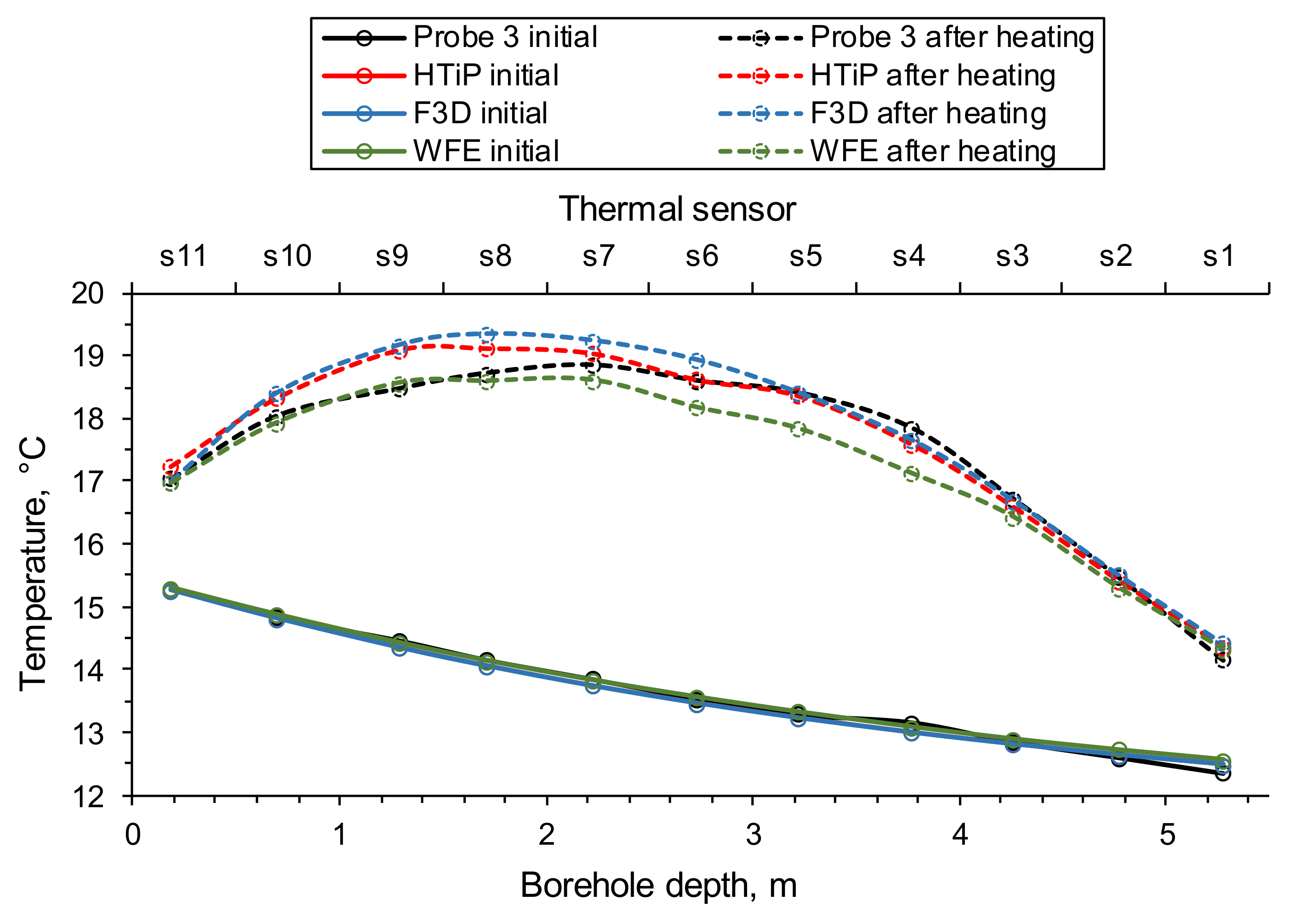
The results of the comparison between rock temperatures at the monitoring borehole, measured in the experiment and simulated approaches, using the HTiP and other models are presented in Figure 9. The temperature readings from 11 sensors (s1–s11) were used for the comparison with the numerical results because they were located closer to the heat source where the thermal signal was stronger. It can be seen that the simulated initial rock temperature at the start of the heating phase (solid lines in colour) achieved a good fit with the measurements (Probe 3 initial), with only small differences at the bottom of the monitoring borehole. The simulated rock temperature after the heating phase (dashed lines in colour) resembled the shape of the measured values, but did not achieve a perfect fit.

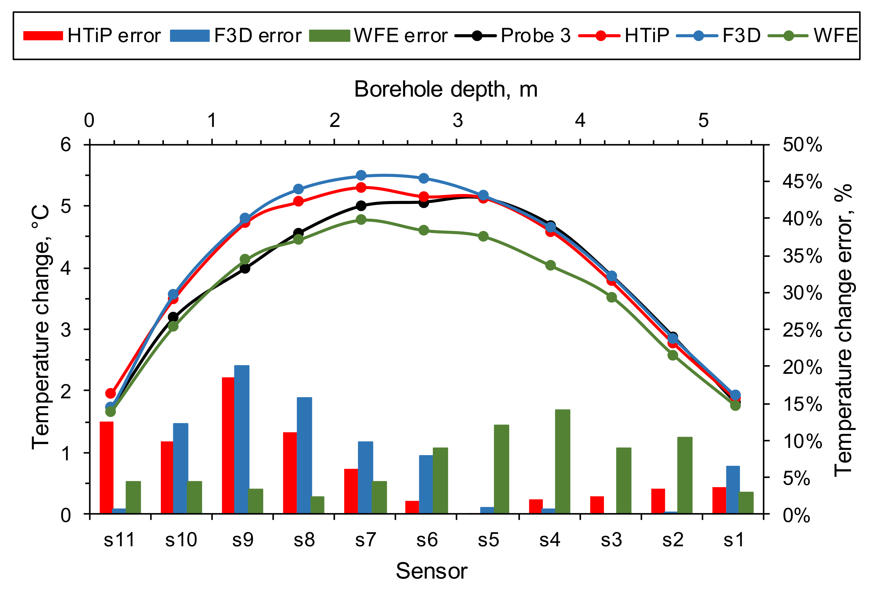
The change in the rock temperature after 21 days of heating was calculated by subtracting the initial temperature from the final temperature. The comparison between the measured and simulated temperature change is shown in Figure 10. Additionally, the error was calculated with Equation (5). The errors for each of the three modelling approaches for each sensor are plotted in Figure 10. It can be seen that both the F3D and HTiP overestimated the temperature increase in the first 2.5 m of the monitoring borehole (sensor s7 to s11) with the highest prediction error occurring at sensor s9, with values of 18% and 20% for the HTiP and F3D models, respectively. The temperature change in the bottom half of the MOBH agreed quite well with the measurements, with the error oscillating between 0% and 4% for both models. A different behaviour was seen for the WFE model as it predicted a similar rock temperature change in the first 1.5 m and last 1 m of the MOBH and underestimated the rock temperature in the middle of the MOBH. The average error for the temperature change estimation was equal to 6.5%, 6.8% and 6.9% for the HTiP, F3D, and WFE models, respectively.

There are several potential reasons for the differences between the predictions of the three models. First, the models differ in regard to the discretisation of the BHE geometry, so the mesh in the direct vicinity of the BHE is also different. Both the HTiP and F3D models have the borehole fully discretised, with grout represented as a three-dimensional domain, whereas the WFE only consists of a single line with grout parameterised in the heat transfer equations. Hence, the similarities between the HTiP and F3D models are smaller compared to the WFE results.

Second, the orientation of the pipes in the BHE (inlet located below the outlet, as depicted in Figure 3a) may have also influenced the differences. The WFE model calculates the grout temperature, which is then prescribed to the line heat source so that the heat is diffused radially in an equal manner in all directions. On the other hand, the geometry of the BHE in the HTiP and F3D models captures the exact location of the pipes and is more realistic. Therefore, the two models give more accurate results with lower error, especially in regard to the outlet temperature.

Finally, the thermal resistance factor between the grout and the rock in the WFE model is calculated according to a simplified approach presented by Al-Khoury et al. [6]. However, the authors of ref. [6] also suggest calibrating the value of the parameter experimentally, which was not the aim of this study. Therefore, the results of the WFE model are only indicative and are used merely for comparison of its efficiency with the main modelling approach. Additionally, the more advanced simplified models, for example, those shown in refs. [9,10] or [12], are recommended.

5.2. Comparison of the Efficiency and Accuracy between the Modelling Approaches

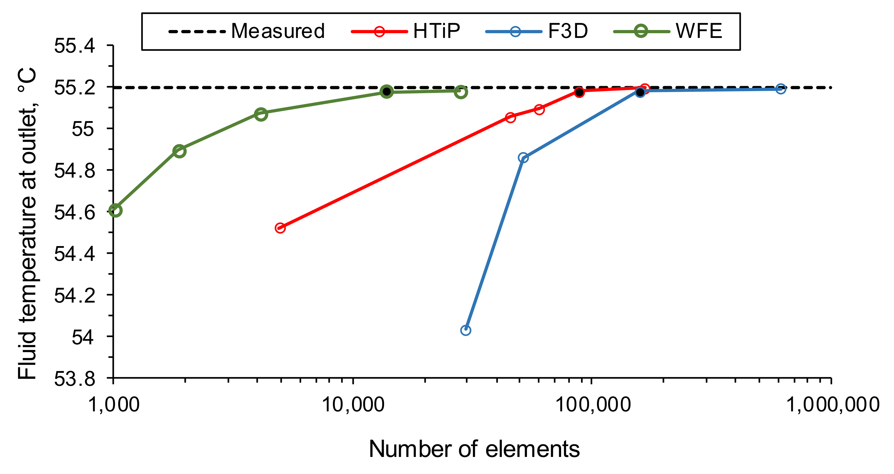
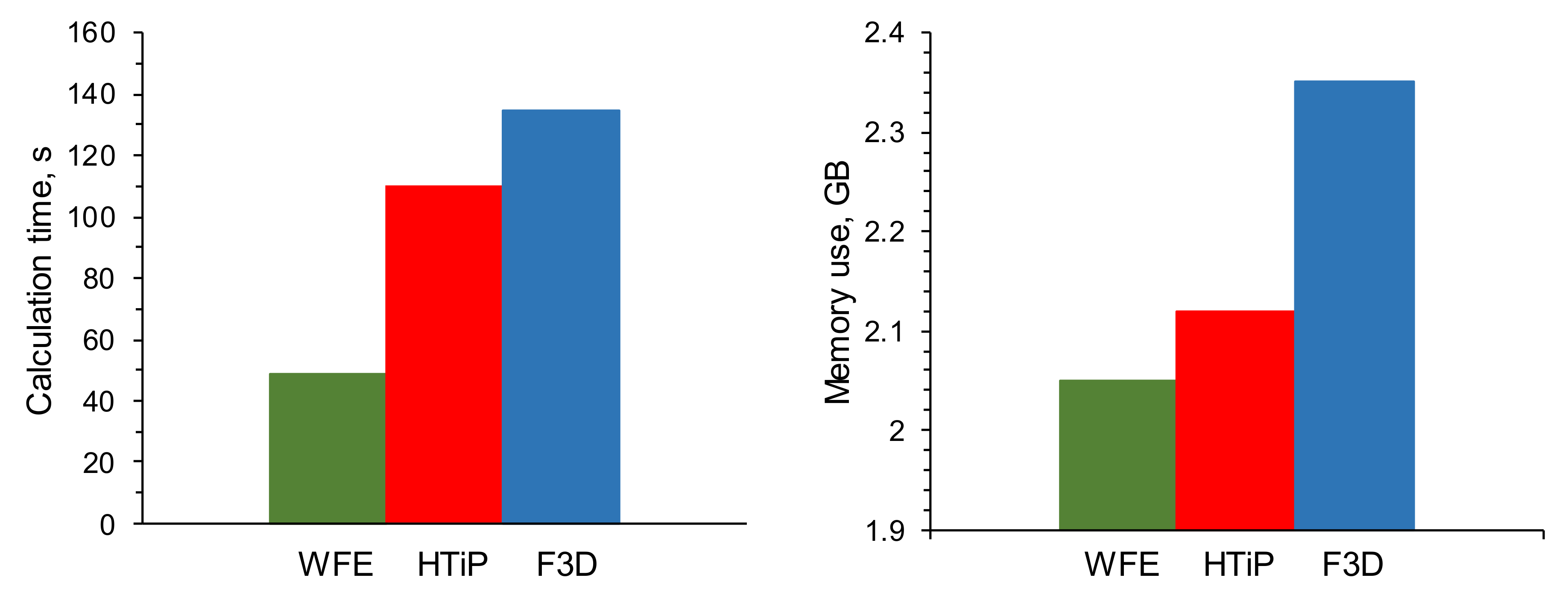
The fastest calculation time and the lowest memory use (see Figure 11a) were achieved by the WFE model by Al-Khoury et al. [6,7] due to the highest order of dimension reduction in the BHE’s geometry discretisation. However, the high computational efficiency led to a lowering in accuracy. The HTiP model was slower than the simplified WFE model. However, the HTiP model gave more accurate results, and the solution time could be further reduced by using an optimised meshing routine. Additionally, the HTiP model was almost as accurate as the fully discretised F3D model by Oberdorfer et al. [17], with the calculation time reduced by almost 20% and the memory use by 10%.

Therefore, fully-discretised models are probably unnecessary, as they involve an increased computational effort, but the accuracy of the solution does not increase considerably. Furthermore, the calculation time achieved by the HTiP model was low enough (see Figure 11) to allow it to be used to simulate the long-term performance of large BTES systems, where the number of BHE can be as high as 200. However, it is recommended that the upscaling of this problem is studied by numerical modelling of large BTES systems using the proposed method.

Additionally, the HTiP model was able to replicate the complicated geometrical arrangements of the BHE, which was difficult to achieve using the WFE model. Hence, the HTiP model is considered to be suitable for simulations of BHE systems with more complex geometries.

5.3. Numerical Model Limitations

There are several uncertainties and limitations of the presented comparison that could have led to differences in temperature change at MOBH between the simulations and the measurements. The differences may arise due to:

• uncertainties and errors in temperature readings,
• errors in the measurement of borehole orientation,
• imperfect contact between the grout and the borehole wall,
• the presence of fractures,
• disturbances in the temperature field,
• simplified fluid flow,
• the influence of weather conditions, or
• inhomogeneity of the rock mass.

The first uncertainty comes from the fact that the difference in observed temperature change may be related to erroneous temperature readings or improper sensor placement in the monitoring borehole. The DS18B20 digital thermometers used for measurements of the rock temperature are characterised by an absolute temperature error of −0.2 ± 0.1 °C within the 10–20 °C temperature measurement range. Even though they had been synchronised to remove the offset before they were installed in the borehole, so that all sensors gave the same temperature readings, there is a possibility that the temperature readings were still inaccurate. Hence, the primary focus is put on a comparison between temperature changes, rather than comparing the absolute values measured. Given the fact that the maximum difference between the temperature change predicted by the models and the measured change was 0.7 °C, the simulated predictions can be considered to be good.

The second uncertainty is related to the measurement of borehole angles. The orientation of both MOBH and EXBH were determined by inserting a 3 m long rod into the borehole and measuring its incline relative to the vertical and horizontal planes. However, if there was any deviation in the deeper section of the boreholes, or if the angles were measured incorrectly, an error in calculation of the simulated rock temperatures would have resulted due to different distances between the heat source and temperature sensors. It was found that a 25% change in the borehole angles would have resulted in a maximum error in simulated rock temperature increase at sensor s7 of +0.5 °C for boreholes oriented closer to each other and −0.7 °C for boreholes spaced further apart.

Next, the imperfect contact between the grout and the rock could have allowed air pockets to be present between them, which would have altered the heat transfer into the rock mass by introducing an additional thermal contact resistance. However, the quality of the contact between the grout and the rock in the in situ experiment was not evaluated.

The similarity between the thermal conductivity measured in the laboratory and in situ confirms that the influence of fractures on the BHE is very minimal or non-existent. Therefore, the identified fractures crossing the borehole were not included in the numerical model for simplification. However, it is still possible that an unidentified fracture was present, running parallel between the EXBH and the MOBH, which would have altered the thermal plume outline. Such fractures may influence the thermal performance of the BHE, as described in ref. [36]. Unfortunately, a detailed mapping of fractures was not done because a layer of shotcrete covered the tunnel walls.

The fifth uncertainty is related to the temperature field around the tunnel network. The tunnel was constructed more than 40 years ago, and it has disturbed the temperature field around it. The exact temperature and air flow in the tunnel network are not known. Additionally, the tunnel is located in an urban area, so there may be an influence of the surrounding buildings on the temperature of the subsurface. It has to be noted that the goal of this study was not to quantify the exact temperature field and its absolute values, but to compare the simulated and measured temperature changes caused by the thermal performance of a short single heat exchanger using the presented numerical modelling approach. Therefore, the small perturbations in the temperature field are of minor importance. Furthermore, the hydration of the grout in the EXBH generated a heat pulse signal that heated up the rock mass. A simple calculation using the exothermic hydration curve given in ref. [37] was performed. The hydration curve estimated the hydration heat to be equal to 5.5 mW/g at its maximum, dissipating with time. The calculation showed that the grout curing process during the 60 h after the injection would produce temperature increases of 0.2 °C and 0.1 °C at the collar and the bottom of the monitoring borehole, respectively. Such temperature increases are much smaller than the temperature increase due to the operation of the BHE; thus, it was ignored in the numerical model.

Next, the heat transfer in the heat exchanger was calculated based on the average velocity of the fluid. However, the fluid flow could be modelled more realistically by coupling the heat transfer with additional pipe flow interface to calculate the fluid velocity and pressure fields to account for pressure losses in the system.

In addition, thermal processes at shallow depths can be strongly influenced by weather conditions, such as air temperature or precipitation [38]. If the water content of the ground is high, it may be necessary to use a numerical modelling approach that, in addition to heat dissipation, is able to also simulate the moisture content transport around the studied object [38,39]. However, in this study, only the outside air temperature was taken into account and the ground was assumed to be dry based on the lack of water outflow from the boreholes.

Lastly, only the average isotropic thermal conductivity of the rock was assumed. The temperature readings could differ if the thermal properties were anisotropic or if their magnitudes differed spatially.

5.4. Results of the Further Investigations Using the HTiP Model

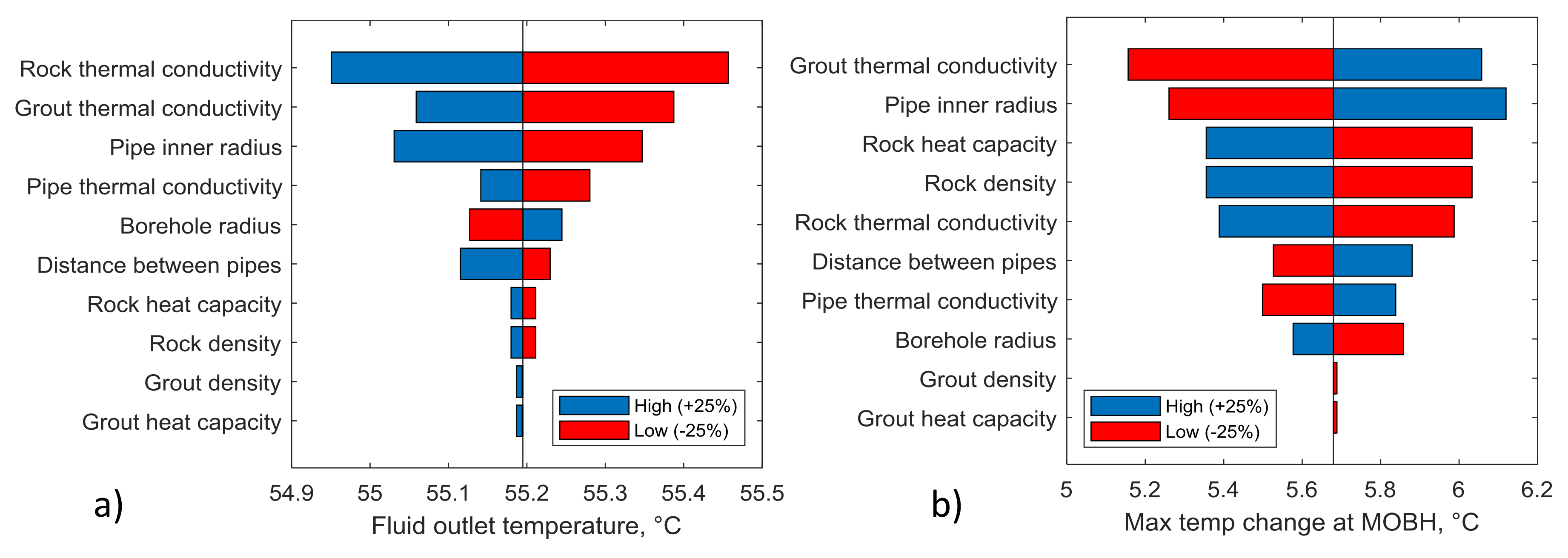
In the sensitivity analysis, the temperature of the fluid at the BHE outlet (Figure 12a) was mostly influenced by the thermal conductivity of the rock. A decrease of 25% in its value resulted in a higher fluid temperature at the outlet, which would lead to a lower fluid temperature drop and less heat being transferred into the surrounding rock mass. Other parameters influencing the fluid temperature drop were the thermal conductivity of the rock, grout, and pipe material—a decrease in their values resulted in a lower fluid temperature drop inside the heat exchanger (an increase in fluid temperature at the outlet). It was also observed that increasing the pipe radius and the distance between pipes in the heat exchanger resulted in a more substantial fluid temperature drop. Parameters such as heat capacity and density of the grout material were found to have low influences on the fluid temperature at the outlet.

The maximum temperature change at the monitoring borehole was mostly influenced by the grout thermal conductivity so that the increase in its value increased the rock temperature change. The same effect was observed for the increased pipe inner radius, the distance between the pipes, and the thermal conductivity of the pipe material. On the other hand, a decrease in rock density, rock heat capacity, rock thermal conductivity, and borehole radius led to more substantial rock temperature changes at the monitoring borehole (see Figure 12b). It was observed that grout heat capacity and grout density do not influence the rock temperature change at the monitoring borehole.

It has to be noted that the effective heat transfer coefficient from Equation (2) is influenced by the inner pipe radius and the thermal conductivity of the pipe. Therefore, an increase in their values will increase the heat transfer coefficient, which will result in a larger temperature drop at the outlet and a larger temperature change in the rock mass.

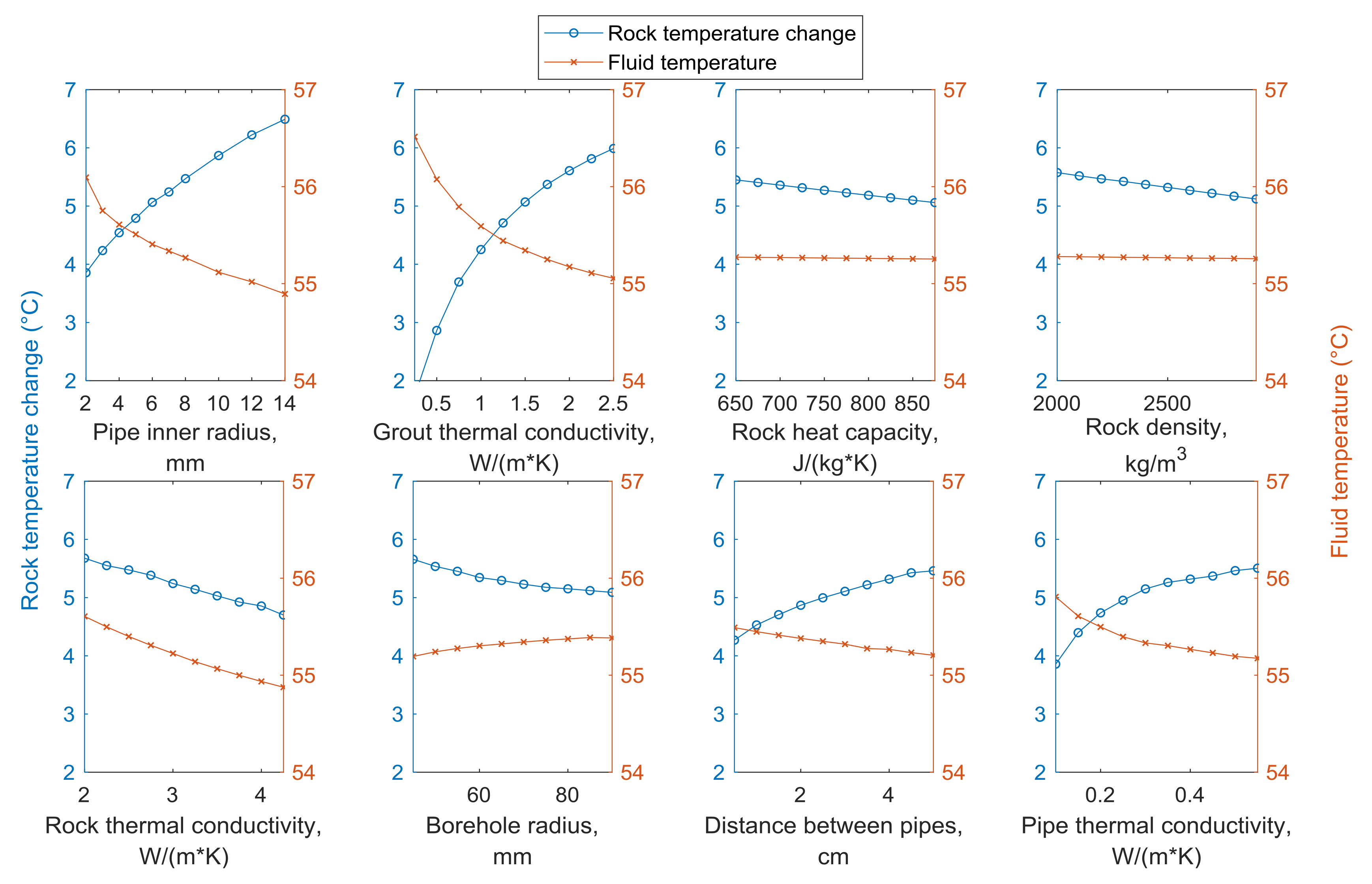
The results of the changes in the fluid outlet temperature and the maximum rock temperature change at MOBH after 21 days of heating are plotted in relation to variations in the selected input parameters (Figure 13). As expected, an increase in the thermal conductivity of the rock resulted in a decrease in both the temperature fluid at the outlet and the rock temperature change at MOBH. The lower fluid temperature at the BHE outlet resulted in more heat being transferred into the rock mass. However, due to the higher thermal conductivity of the rock, the thermal energy was conducted faster, which resulted in a lower temperature change in the rock at a 1 m distance.

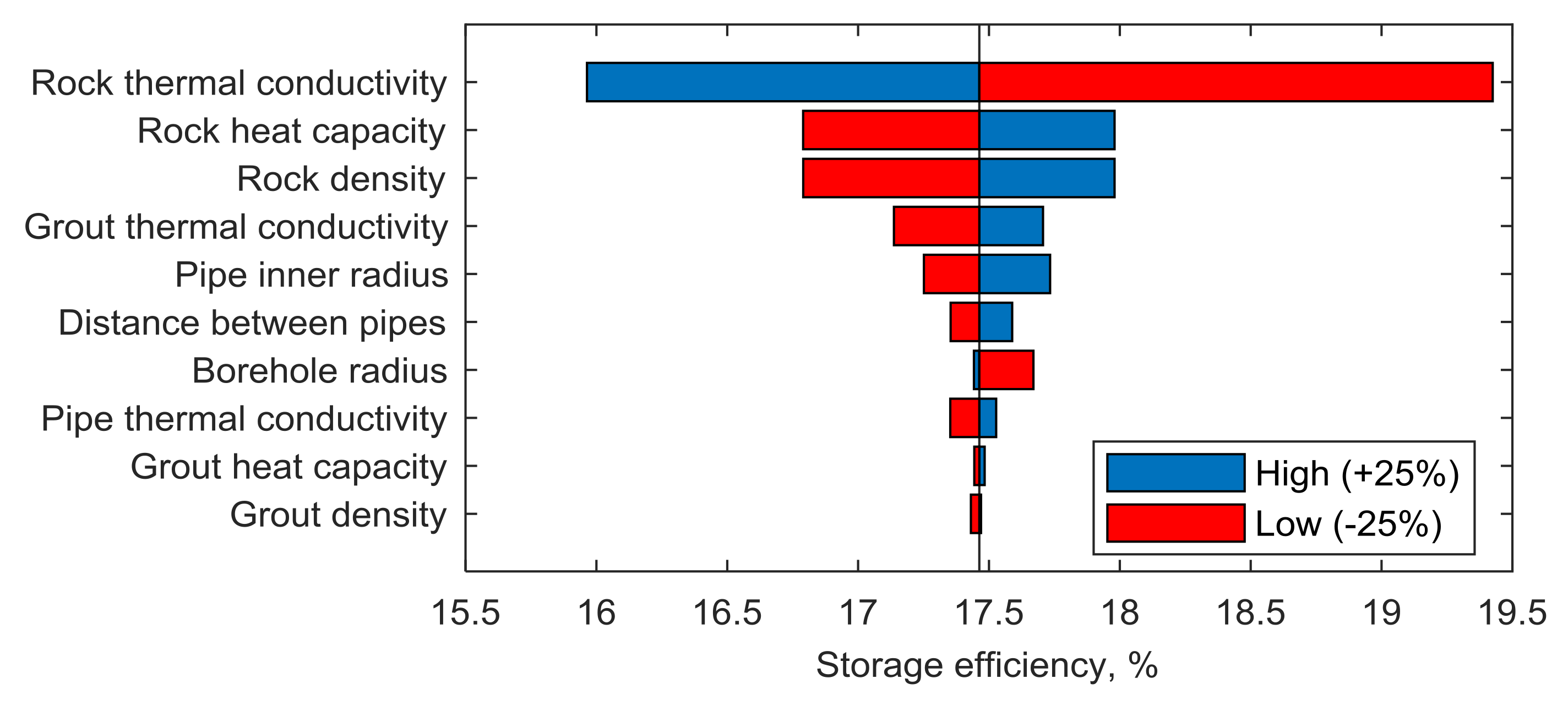
The results of the storage efficiency sensitivity assessment (Figure 14) showed that the following characteristics of the BHE set-up are required if the goal is an increase in the storage efficiency of the BHE or BTES (the most influential parameters are on the top):

• low rock thermal conductivity,
• high rock heat capacity,
• high rock density,
• high grout thermal conductivity,
• high pipe inner radius,
• high distance between the pipes (shank spacing), and
• low borehole radius.

Out of the abovementioned parameters, the first three explicitly formulate the thermal diffusivity of the rock, $\alpha =\frac{{\mathsf{\lambda }}_r}{C_r·{\rho }_r}$, and their magnitudes explicitly state that the low thermal diffusivity of rock is essential for increasing the storage efficiency. Thus, the thermal properties of rock relative to its use as a storage medium are the most influential factors and can only be influenced during the process of site selection for the project. All the other parameters from the list can be tweaked to maximise the storage performance of a BTES system in the detailed engineering design stage. The final values used for the BTES setup should follow a rigorous optimisation process based on technical and economic constraints.

The obtained results correspond well with the findings from ref. [18], which indicated that the borehole’s thermal resistance could be lowered by decreasing the borehole’s radius, increasing the distance between pipes, increasing the inner pipe radius, and increasing the thermal conductivity of the grout and the pipe material. It has to be noted that by increasing the pipe radius, the thermal shortcutting effect (heat exchange between the inlet and outlet pipe) will be more pronounced. The authors of ref. [18] stated that there is an optimal pipe radius that will maximise the heat transfer through the borehole wall with minimal thermal shortcutting. Furthermore, the high influence of the thermal conductivity of the rock and grout on storage efficiency is in agreement with the results of the sensitivity analysis presented in ref. [40].

Another essential parameter with a high influence on the result, which was not included in the sensitivity analysis, is the fluid velocity. A previous study by the current authors [23] found that a decrease in fluid velocity increases the temperature drop of the fluid, at least until the value corresponding to the fluid flow being in the turbulent regime.

6. Conclusions

Long-term thermal energy injection into crystalline rock using a single borehole heat exchanger (BHE) was investigated using the proposed Heat Transfer in Pipes (HTiP) finite element numerical model. The goal of this study was to validate the proposed methodology and compare it with other methods from the literature to evaluate its applicability for numerical simulations of seasonal thermal energy storage in rocks using boreholes. The numerical model was validated by an in situ experiment conducted in an underground research tunnel.

The HTiP numerical model simulated the behaviour of the BHE accurately. It was faster to calculate than the full 3D model, but slower than the weak form equations model. However, the HTiP model was able to replicate the complicated geometrical arrangements of the BHE and is considered more suitable for simulations of BHE systems with more complex geometries.

Based on the sensitivity analysis of thermal energy storage in crystalline rock, low diffusivity in the rock used as a storage medium is essential for maximising the storage efficiency of a single BHE. Additionally, the following characteristics of the BHE are preferred to achieve large seasonal storage performance: high grout thermal conductivity, large pipe radius and distance between the pipes, low borehole radius, and high pipe material thermal conductivity.