Article

Mitigating Household Energy Poverty through Energy Expenditure Affordability Algorithm in a Smart Grid

Electrical and Electronics Engineering Science, University of Johannesburg, Johannesburg 2006, South Africa
*
Author to whom correspondence should be addressed.
Energies 2018, 11(4), 947; https://doi.org/10.3390/en11040947
Submission received: 12 March 2018 / Revised: 11 April 2018 / Accepted: 12 April 2018 / Published: 16 April 2018
(This article belongs to the Special Issue Energy Efficient and Smart Cities)

Abstract

:
One of the criteria for measuring household energy poverty is the percentage of the household’s income spent on energy expenses. In this work, an autonomous income-based energy scheduling demand side management (DSM) technique called energy expenditure affordability algorithm (EEAA) is proposed to ensure that household energy expenditure is below the nation’s approved energy expenditure threshold. The EEAA problem was formulated as a mixed integer linear programming (MILP) problem and verified with real household data collected from families living in bachelor flats in Johannesburg, South Africa. Consumer preferences and satisfaction were enhanced by using the dynamic time warping (DTW) technique to minimize the distance between nominal and EEAA load profiles. Furthermore, the effects of distributed energy generation (DEG) and distributed energy storage (DES) were also investigated in light of energy expenditure affordability for improved consumer-friendly and satisfying DSM. The EEAA-DSM technique is shown to reduce household energy expenditure below the energy expenditure threshold, offering energy expenditure affordability as well as utility grid peak demand reduction (PDR). Furthermore, grid reliability and sustainability, environmental preservation and gendered energy poverty are consequential benefits of the EEAA. It also offered the households considered an average financial savings from 12% to 82%, depending on the level of implementation of distributed storage and generation to the consumer’s local energy mix.

1. Introduction

Household energy poverty is one of the major approaches to defining energy poverty [1]. It can deprive affected households of other essential goods and services needed for optimum socioeconomic activities [1,2,3]. Energy expenditure is a recurrent monthly cost for households, and the demand for electricity by consumers is generally inelastic with respect to household income. However, the percentage of household income spent on energy is one of the indicators of energy poverty. The government in each nation determines the energy expenditure threshold for residents based on certain factors of its economy. Any household that spends above the approved nation’s energy expenditure threshold is considered to be energy poor [1,2,3].
The growth in electricity demand challenges the traditional grid due to the increasing numbers of appliances, gadgets, equipment and machineries that need to be powered. However, demand side management (DSM) programmes can be used to achieve (near) balance of energy demand and supply in the smart grid. Further enhancement to both DSM and consumer satisfaction can also be achieved by introducing distributed energy generation (DEG), distributed energy storage (DES) and distributed energy generation and storage (DEGS) systems [4,5,6,7,8]. DEG, DES, and DEGS will be collectively referred to as alternative energy supply system (AESS) in this article. Hence, an AESS can be any of DEG (e.g., solar energy, wind energy, biomass, etc.), DES (e.g., batteries, fuel cells, etc.) or DEGS. Therefore, an AESS comprises of devices that offer alternate solutions to energy supply to consumers through distributed generation, and/or distributed storage.
Despite the research that abounds in the literature on DSM to reduce energy cost to consumers [7,8,9,10,11,12,13,14,15,16], as far as the authors are concerned, to date, none has investigated optimising energy expenditure in the context of household income in order to mitigate household energy poverty. Therefore, energy management technique is introduced to reduce both electricity consumption and monthly energy expenditure by consumers. In this article, a DSM technique called energy expenditure affordability algorithm (EEAA) is proposed to reduce household spending on energy consumption above the approved energy expenditure threshold under a time-of-use (TOU) pricing scenario. It is common practice to have DSM algorithms to attempt to minimise consumer discomfort through their algorithms [6,7,8,9,10,11,13,14,15], but the level of discomfort must be greatly minimal or negligibly minimal for consumers to accept it and to be willing to deploy it on their premises. Some of the literature, however, considered consumers’ comfort in their proposed DSM algorithm, but did not offer energy expenditure affordability, since a reduced cost does not mean cost affordability. However, affordability, which is dependent on income, is the essence of this work. The work in [13] is further limited as consumer’s comfort is constrained by the behaviour of others in the game, while [14] allowed some stubborn players to take decisions that can affect the comfort of other players in the game.
Furthermore, the proposed EEAA does not offer only reduced energy expenditure, like other algorithms, but also affordable energy expenditure, which can mitigate household energy poverty and enhance the consumer’s comfort by making sure that the optimised load profile is one with the least distance from the nominal load profile, thus ensuring the lowest cost to the consumer. Also, each consumer optimises its energy consumption and expenditure independently in a distributed manner, without the knowledge of other consumers in the network, thereby enhancing consumer privacy and security in a smart grid. The challenge of gendered energy poverty, which often results whenever energy expenditure is not affordable by households, would also be mitigated by the EEAA implementation. All these features make the proposed EEAA novel contribution unique in DSM and household energy poverty mitigation.
The growing demand during traditional peak periods has necessitated the introduction of TOU pricing by the utility provider in order to force some peak demand to be shifted from traditional/existing peak periods to traditional non-peak periods. TOU-based DSM programmes set electricity prices (tariffs) according to the time of the day and the season of the year when the energy is consumed. The TOU energy tariffs for peak periods are higher than for non-peak periods. Usually, the higher the estimated consumer demand at a given time/period, the higher the tariff for such a time/period, and consequently, the higher the energy expenditure at such time/period by the consumers. The utility provider usually communicates the approved TOU tariff to customers in advance.
Monthly energy expenditure comes from the cumulative daily energy consumption by all the appliances in use in a household in the month under consideration. Therefore, energy consumption by smart appliances connected within a smart home to a smart meter is optimised to ensure that the household’s energy expenditure is not more than the approved national energy expenditure threshold, in the context of the household’s income. An EEAA device with built-in EEAA is proposed to be installed into the smart meters of consumers. The proposed EEAA technique involves a mathematical optimisation problem formulated as the mixed integer linear programming (MILP) problem [17], due to the type of functions involved in its formulation.
This study has shown that incorporating an EEAA device into smart meters will minimize energy poverty at household levels, will offer better financial savings and planning, energy savings, and demand satisfaction, and will encourage the penetration of AESS in consumer premises. The utility can also effectively plan for its energy generation and distribution networks. Furthermore, the government would have fewer energy-poor households in the country, depending on the level of integration of the EEAA algorithm in consumer premises (especially low-income and middle-income households).
The rest of the paper is organized as follows. An overview of household income and energy expenditure is presented in Section 2; EEAA architecture and problem formulation are discussed in Section 3; the numerical results are presented in Section 4; and finally, conclusions are drawn in Section 5.

2. Household Income and Energy Expenditure Affordability

Electricity consumption by households is largely dependent on household income, lifestyle, and appliances owned [18], but the percentage of income spent on energy expenditure is a primary concern in this work. Energy expenditure is important, because it is one of the indicators of household energy poverty.
The energy expenditure threshold is the approved maximum income-dependent amount that a household should spend on energy costs. It is usually set by the government of any nation, and it is 10% to 15% of household income [2,3,19]. For example, the Department of Energy (DoE) in South Africa has chosen 10% as energy expenditure threshold in the country [2]. Therefore, any household in South Africa that spends more than 10% of its income on paying for energy is regarded as energy poor. The DoE, through a nationwide survey, found that South African households spend an average of 14% of their income on energy expenditure, with the majority found among low- and medium-income households [2]. Similarly, in developed [19,20,21] and developing [2,18,22] countries, the population that spends above the nation’s expenditure threshold is usually found among low- and middle-income earners. Table 1 [2] gives a summary of the income class and the average energy expenditure by South African households, derived from a national survey conducted by DoE, South Africa. The lower quintile and the 2nd quintile fall in the low-income class, the 3rd and 4th quintiles fall in the middle-income class, while the upper quintile falls in the upper-income class [2,23]. Table 1 shows that energy expenditure for most of the lower- and middle-income earners was above the approved energy expenditure threshold for the nation.
The number of households connected to electricity supply from the mains electricity has increased from 77.1% in 2002 to 84.2% in 2016, thereby making more households use mains electricity for cooking, especially in the Northern Cape, Free State, Western Cape, and Gauteng provinces of South Africa [24]. However, only a slight increase is noticed in provinces such as Limpopo, the Eastern Cape, and Mpumalanga, where alternative fuels (e.g., wood) are more affordable and accessible for households. It therefore implies that increased access to electricity can only result in reduced household energy poverty, provided that the energy expenditure is affordable within a household’s income. Hence, the need for a solution like the proposed EEAA, which could ensure affordable energy expenditure to all households with access to electricity.
Energy expenditure affordability is therefore defined as the ability of a consumer to meet its total energy demand below the approved energy expenditure threshold without depriving itself of other basic needs of life, such as food, health, clothing, shelter, education, etc. This paper therefore proposes the EEAA for consumers, so that they would spend less than the approved energy expenditure threshold with consideration for consumer’s comfort. The financial savings derived from EEAA could also impact the socioeconomic lifestyles of the households.
The South African TOU energy tariff [25,26] was used to test the EEAA algorithm for selected consumers.

3. EEAA Framework for DSM in Smart Homes

In this section, the proposed EEAA framework for TOU smart homes, the system description or architecture, and the mathematical problem formulation, are presented. The EEAA optimises consumer energy consumption and expenditure by optimising daily energy consumption and expenditure in the household, based on household income, electricity tariff and availability of an AESS.

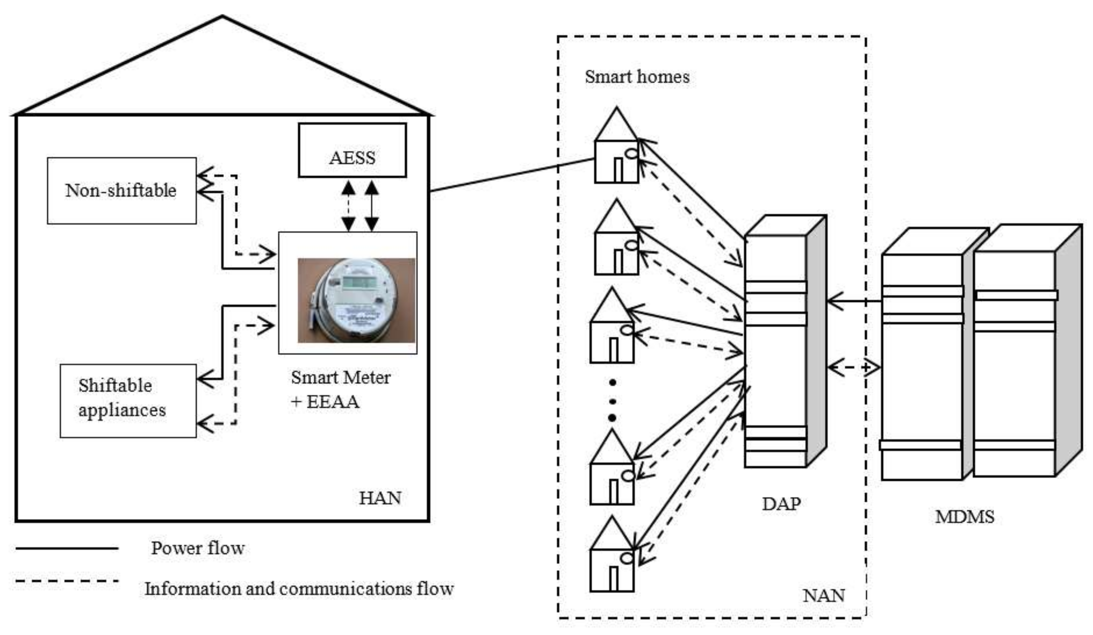
3.1. Description of the EEAA Architecture

Consumer appliances in the smart home are connected to the smart meter, which serves as a link between the smart home and the data aggregation point (DAP) at the utility end. Each household is assumed to have an EEAA device installed into the smart meter or in-home display (IHD) for optimisation of energy consumption and expenditure within the limits of affordability. These smart homes communicate bidirectionally with the utility through the DAP and meter data management system (MDMS) in the smart grid. Enabling home area network (HAN) and neighbourhood area network (NAN) are assumed to exist in the smart grid for effective communication between consumers and the utility provider. The communication technologies employed for HAN, NAN, and wide area network (WAN) in a smart grid can be a wired (e.g., ethernet, power line communication (PLC), fibre optic, digital subscriber line (DSL), etc.) wireless (e.g., Wi-Fi, Bluetooth, ZigBee, WiMAX, Z-wave, DASH7, cellular, satellite, etc.) or hybrid (e.g., INSTEON, X10, etc.) communication technologies depending on the characteristics of the network environment [27,28]. The proposed EEAA system architecture is illustrated in Figure 1.
The smart appliances are categorised into non-shiftable (non-schedulable) appliances and shiftable (schedulable) smart appliances. Power-shiftable and time-shiftable smart appliances are also jointly categorised together as shiftable appliances in this paper.
Work is ongoing to embed the EEAA into an energy controller microchip that can be installed into a consumer’s smart meter. The microchip will be a low-cost, non-intrusive, load management device that can easily be installed into smart meters. The EEAA device is proposed to function effectively in either a wireless or wired communication environment.
In order to ensure privacy and security of household data (consumption and income) under the proposed EEAA architecture, a cryptographic scheme that anonymises data before sending to DAP was included. Details of this are presented in another paper.

3.2. EEAA Mathematical Formulation

The proposed EEAA model can be described as an optimisation problem that optimises daily energy consumption and expenditure for households through their smart meters according to their proposed monthly budget for energy expenditure, which is household income-dependent.
Let the non-shiftable and shiftable smart appliances be i I and h , respectively, in customer a A household, where A = { 1 , 2 , , A } , where the set of all smart appliances is G = I for g = { i , h } , g G . The total hourly energy consumed x a , t at time t T by all non-shiftable and shiftable smart appliances in the home is given by [6]:
x a , t = i I x a , i , t + h x a , h , t ,   a A ,   t T ,
where x a , i , t is the energy consumed by a non-shiftable smart appliance, and x a , h , t is the energy consumed by a shiftable smart appliance owned by consumer a A at timeslot t T , where T = [1, 2, …, ȶ ].
Therefore, let the feasible periods of operation T a , i and T a , h of any non-shiftable and shiftable smart appliance in the household have operation start times t a , i s and t a , h s and end times t a , i e and t a , h e , respectively, where T a , i = { t | t a , i s t t a , i e } ,   i I and T a , h = { t | t a , h s t t a , h e } ,   h . Then, total energy e a , g consumed by a non-shiftable and a shiftable smart appliance in the smart home during their feasible periods of operations is given by
e a , g = { t a , g s t a , g e x a , g , t ,   t T ,   g = { i , h } ,   g G 0 ,   t T \ T a , g ,   T a , g = { T a , i , T a , h } ,   g = { i , h } ,   g G ,
where T a , g = { T a , i , T a , h } is the feasible operation period for all shiftable and non-shiftable smart appliances in consumer a A premise. The power level constraint for each appliance is given as
x a , g m i n x a , g , t x a , g m a x ,   t T a , g ,   g = { i , h } ,   g ,   a A ,
where x a , g m i n and x a , g m a x defines the minimum power levels (OFF or standby mode) and maximum power levels for each smart appliance. The minimum power level is constrained as x a , g m i n 0 . Therefore, the energy balance is given by (4) and summarised in (5):
x t = a A ( i I e a , i , t + h e a , h , t ) ,   i ,   h ,   t ,
x t = a A g G e a , g , t ,   g = { i , h } ,   a ,   t .
Furthermore, the hourly load in a household is bounded between the consumption by the non-shiftable appliances and the maximum household load x a m a x , which is dependent on the fuse/line capacity or as determined by the utility for each household and is given by
i I x a , i , t x a , t x a m a x ,   a A ,   t T .
The load vector x for all households in the smart grid is given as x = [ x 1 ,   x 2 , ,   x A ] , and the daily load vector x a for each consumer a is given as x a = [ x a , 1 , x a , 2 , , x a , ȶ ] , while the total daily load for a consumer x a is expressed as:
x a = t T x a , t .
The consumption pattern per household for each non-shiftable smart appliance x a , i = [ x a , i , 1 ,   x a , i , 2 , , x a , i , ȶ ] and shiftable smart appliances x a , h = [ x a , h , 1 x a , h , 2 ,   ,   x a , h , ȶ ] can be further expressed by the diagonal matrices (8) and (9) respectively:
x a , i = [ x a , i , 1 0 0 x a , i , ȶ ] ,   i I .
x a , h = [ x a , h , 1 0 0 x a , h , ȶ ] ,   h
Also, the nominal power consumption matrices for each smart appliance i I and h are given as w a , i = [ w a , i , 1 , w a , i , 2 , , w a , i , ȶ ] and w a , h = [ w a , h , 1 , w a , h , 2 , , w a , h , ȶ ] , respectively. Therefore, for shiftable smart appliances, the power consumption matrix denoted by W a , h is the circular shifts of w a , h , expressed as
W a , h = [ w a , h , 1 w a , h , ȶ w a , h , 2 w a , h , 1   w a , h , 3 w a , h , 2 w a , h , 4 w a , h , 3 w a , h , ȶ w a , h , ȶ 1   w a , h , 2 w a , h , 1 ] .
The switching state of each smart appliance can be represented by a binary integer vector s , since the smart appliances were assumed to take on either 0 or 1 switching states per time:
s = [ s 1 ,   s 2 ,   s 3 ,   ,   s ȶ ] ,   s { 0 , 1 } ȶ x 1 .
The switching vector s chooses the optimal power consumption column from W a , h in (10) for the shiftable appliances at any time t T with respect to energy prices. Therefore, the energy consumption vector for non-shiftable and shiftable smart appliances are given by (12) and (13) respectively:
x a , i = w a , i s a , i ,   i I ,
x a , h = W a , h s a , h ,   t s a , h , t = 1 ,   h ,   t T .
Consumer preference or satisfaction with the EEAA algorithm is further enhanced by minimising the “distance” between the nominal and scheduled load profiles of the consumer, which is an important concern of most consumers with DSM algorithms. Therefore, a technique called dynamic time warping (DTW) [29,30] is employed in this work to measure and limit the “distance” between the nominal and the scheduled consumption pattern series during optimisation. DTW is a mature and robust technique for finding optimal alignment between two given time-dependent sequences with non-linear time normalization under certain restrictions [29,30]. It has applications in many fields of science and technology including smart grid [31,32].
If there are two consumption preference vectors x ˜ a and x ¯ a , which are time series patterns for a household a A , where x ˜ a = { x ˜ a , 1 ,   x ˜ a , 2 ,   ,   x ˜ a , t , , x ˜ a , ȶ } and x ¯ a = { x ¯ a , 1 ,   x ¯ a , 2 ,   , x ¯ a , t , ,   x ¯ a , ȶ } , then the two time series sequences x ˜ a and x ¯ a can be warped non-linearly, so that the warping cost can be minimised, which will minimise dissatisfaction of the households due to consumption scheduling. Therefore, the warping cost δ ¯ a t = D T W ( v , u ) between a subsequence of vectors x ˜ a and x ¯ a with first time slots v and u , respectively, can be given as
δ ¯ a t = | x ˜ a , v x ¯ a , u | + m i n ( D T W ( v 1 , u ) D T W ( v , u 1 ) D T W ( v 1 ,   u 1 ) ) .
The value of δ ¯ a t is kept as low as possible in order to obtain the least normalized “distance” between a nominal and scheduled consumption pattern series by further calculating the normalized Euclidean distance. Although there are other time series similarity techniques such as artificial neutral networks (ANN) and hidden Markov model (HMM), DTW was chosen due to its simplicity, speed of analysis, and reduced computational complexity.
The presence of AESS is assumed in consumer premises, which is one of the expected features of the future smart grid. In a DSM + EEAA + DEG (DADG) scenario, where a non-dispatchable generator is owned by consumer, a A , it produces g a , t amount of energy at time t . A non-dispatchable solar energy generator (e.g., roof-top solar panel) with intermittent solar resources is assumed in this work.
Also, in a DSM + EEAA + DES (DADS) scenario, the consumer is assumed to possess DES only. Let the battery daily energy storage scheduling vector, b a = [ b a , 1 , b a , 2 , ,   b a , t , ,   b a , ȶ ] , where b a , t = b a , t + b a , t , b a , t + ,   b a , t 0 , given that b a , t + and b a , t are energy charging and discharging profiles, respectively. The charging efficiency β a + and discharging efficiency β a fulfil conditions 0 < β a + 1 and β a 1 , respectively. Therefore [8],
β a b a , t b a m a x , a A ,   t T ,
where b a m a x is the maximum charging/discharging rate. The energy leakage rate λ a constrained by 0 < λ a 1 , the previous charge level q a , t 1 at time t 1 , the present time t charge level q a , t , initial charge level q a , t 0 and the battery capacity b a , c a p , are related by [8]
q a , t 1 ( 1 λ a ) β a b a , t b a , c a p q a , t 1 ( 1 λ a ) .
q a , t = q a , t 0 ( 1 λ a , t ) + t = t 0 t λ a , t t 0 β a b a , t , a A .
In this paper, uncertainties regarding energy production from solar energy were mitigated with the inclusion of energy storage (in-home batteries) in the design. The batteries are charged from solar energy generation during the day, and the stored energy is supplied for consumer’s consumption at periods of high energy price (peak demand or critical peak demand) from the utility grid. However, such mitigation can be enhanced in the future through grid-connection and enhanced weather forecast.
Furthermore, in the DSM + EEAA + DEGS (DADGS) scenario, the consumer is assumed to possess both DEG and DES. While the DSM + EEAA (DA) scenario involves DSM with EEAA optimisation only, but without AESS, and the non-DSM (ND) scenario is the nominal energy consumption of the consumer without any form of DSM, EEAA, nor AESS.
Household energy expenditure is a function of the energy consumption of all appliances, x a , g , t , household monthly income I a , TOU tariff P t at time t T , number of days n in a month, and the amount of energy taken from AESS, if available. In order to ensure affordable energy expenditure and to have more energy-rich households in a country, it is necessary to constrain energy expenditure below the nation’s expenditure threshold. Therefore, the actual monthly energy expenditure C a , m and monthly energy expenditure threshold C a , m , m a x are related by
0 < C a , m C a , m , m a x ,   a A .
The monthly energy expenditure threshold C a , m , m a x for a consumer is constrained by the nation’s approved energy expenditure threshold coefficient k and monthly income I a , and is given as
C a , m , m a x k I a ,   a A .
Initial daily maximum energy expenditure C a , d , m a x is obtained using
C a , d , m a x = C a , m , m a x n   = k I a n .
Hence, the consumer is not expected to spend more than C a , d , m a x daily on energy expenditure, for mathematical simplicity. The actual total daily energy expenditure C a , d due to optimised consumption is constrained as C a , d C a , d , m a x . The daily energy expenditure savings C a , d , s , given as C a , d , s = C a , d , m a x C a , d , are brought forward to the next day, and added to the initial C a , d , m a x of the next day. Therefore, the next day C a , d , m a x = initial   C a , d , m a x + C a , d 1 , s , where C a , d 1 , s is the energy expenditure savings from the previous day. However, C a , d is found in terms of the household’s hourly energy expenditure C a , t , as follows
C a , d = C a , 1 + C a , 2 + +   C a , t = t T C a , t ,   a .
The actual monthly energy expenditure C a , m is expressed as the summation of the daily energy expenditure C a , d for the month under consideration from the first day of the month m f to the last day of the month m l , and is given as
C a , m = m f m l C a , d = m f m l t = 1 t = ȶ C a , t ,   ,   a A .
An hourly TOU tariff system is considered in this work, and is represented by the tariff vector matrix P, where P = [ P 1 , P 2 , , P t , , P ȶ ] , t T , with each element in P defined according to information obtained from the utility provider in [25,26].
Energy expenditure in a household at any time t T is a function of total energy consumed x a , g , t , the presence of DEG, DES or both, and applicable TOU tariff P t . Therefore, the hourly cost of load profiles for scenarios DA, DADG, DADS, and DADGS are respectively
C D A , a , t ( L D A , a , t ) = P t x D A , a , g , t + δ ¯ D A , a t ,   a A ,   t ,
C D G , a , t ( L D G , a , t ) = P t ( x D G , a , g , t g D G , a , t ) + δ ¯ D G , a t ,   a A ,   t ,
C D S , a , t ( L D S , a , t ) = P t ( x D S , a , g , t b D S , a , t ) + δ ¯ D S , a t ,   a A ,   t ,
C D G S , a , t ( L D G S , a , t ) = P t ( x D S G , a , g , t + b D G S , a , t g D G S , a , t ) + δ ¯ D G S , a t ,   a ,   t .
The cost functions (23)–(26) were optimised for each household accordingly.

3.3. EEAA Optimisation Problem

The EEAA optimisation problem can be formulated as an MILP problem using the branch-and-bound method [17] implemented in CPLEX [33] for the DA, DADG, DADS, and DADGS scenarios in (27)–(30), respectively, as follows:
min L D A , a , t , δ ¯ a t C D A , a , t ( L D A , a , t ) , s.t. ( 1 ) ( 14 ) ,   ( 18 ) ( 23 ) .
min L D G , a , t , δ ¯ a t C D G , a , t ( L D G , a , t ) , s.t. ( 1 ) ( 14 ) ,   ( 18 ) ( 22 ) ,   ( 24 ) .
min L D S , a , t , δ ¯ a t C D S , a , t ( L D S , a , t ) , s.t. ( 1 ) ( 22 ) ,   ( 25 ) .
min L D G S , a , t , δ ¯ a t C D G S , a , t ( L D G S , a , t ) , s.t. ( 1 ) ( 22 ) ,   ( 26 ) .
The EEAA algorithm was designed to solve the above problems in (27)–(30) for each household and the numerical results are found in the next section.

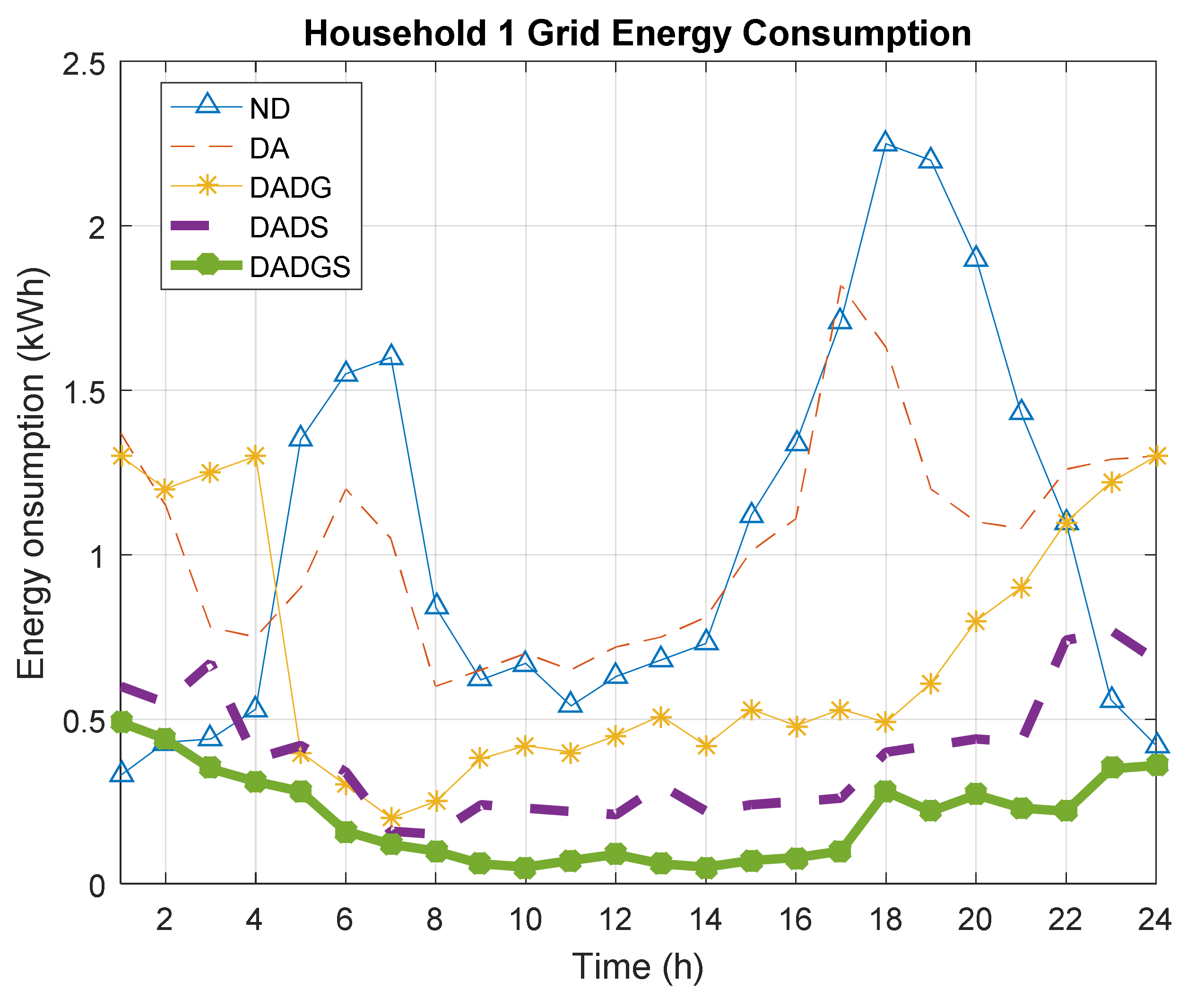
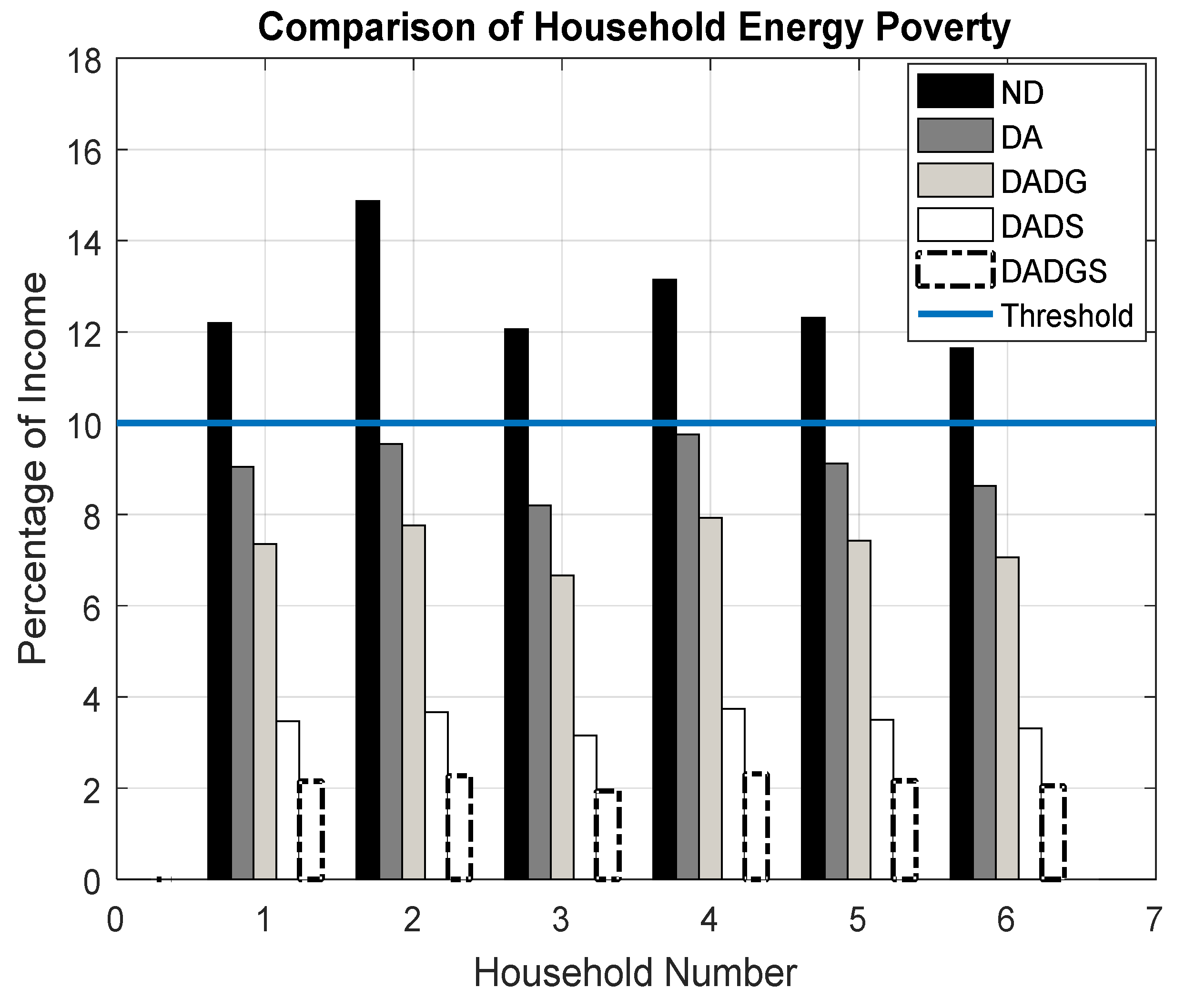
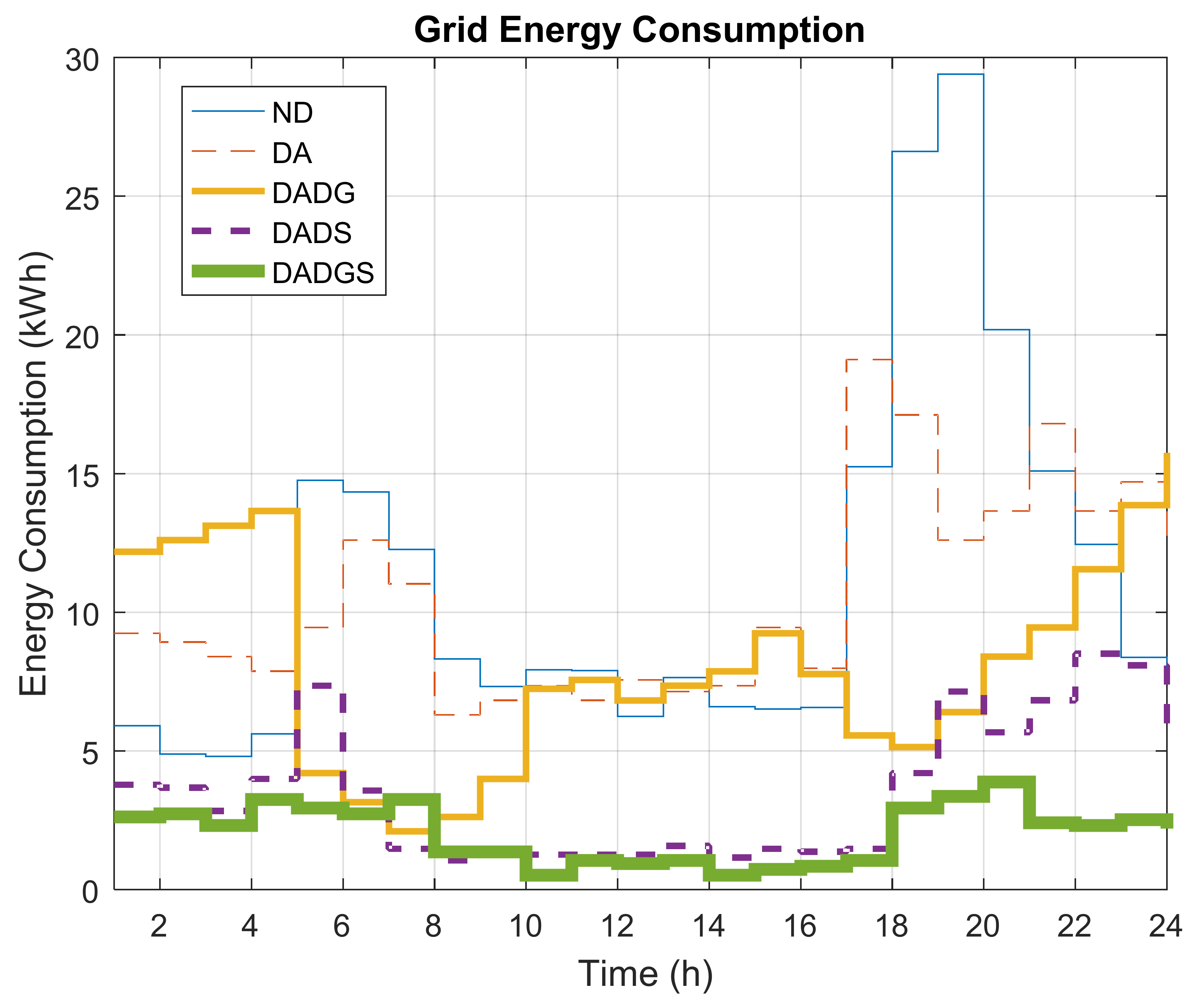
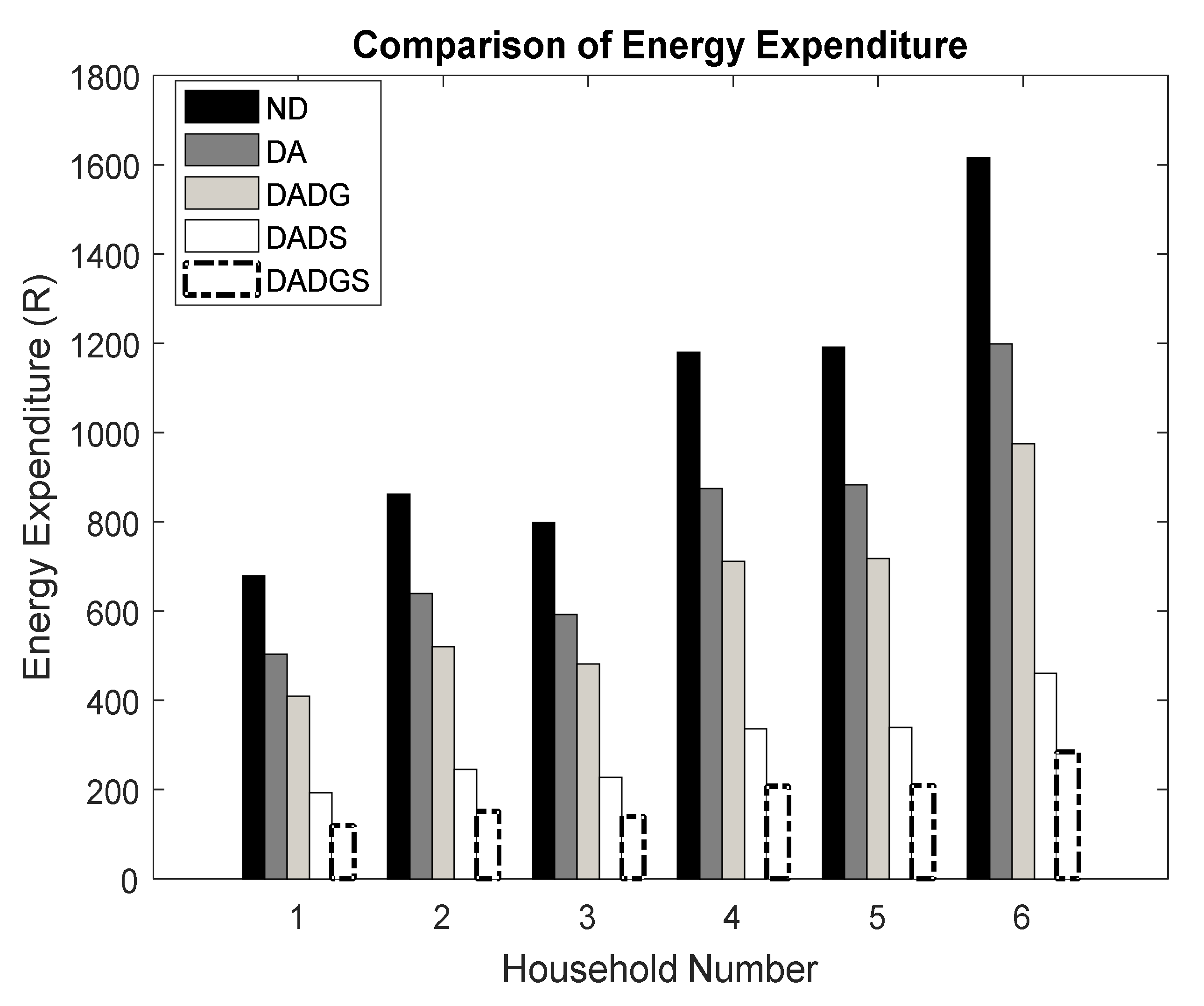
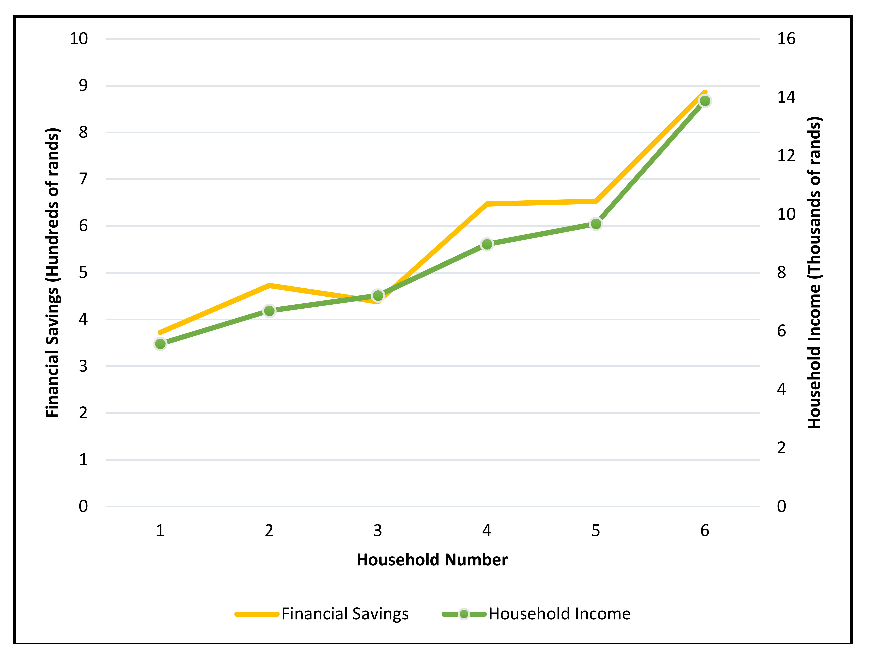
4. Numerical Results and Discussion

The proposed EEAA was tested on households living in a building comprising six bachelor flats in Johannesburg, South Africa. Their consumption data in summer and in winter were collected using the Efergy Engage Elite Hub [34], which was installed on their distribution board. The load profile obtained was used as day-ahead data, and fed into the EEAA for next day optimisation. Also, information on each household income (rounded up to the nearest whole number), size, initial energy expenditure and interest (as inquired from them) in adoption of the proposed EEAA technology is presented in Table 2. Each bachelor flat is considered a household, because each is inhabited by a family. Their individual initial average energy expenditure was above the 10% threshold, hence they are considered as energy-poor households, and are suitable for this study. The households were not chosen primarily on income basis, but income information was obtained from the households living in our experimental building where the Efergy equipment was installed. Also, since their consent to the technologies was positive, that is, either “Strongly Agree” or “Agree” (as shown in Table 2), it means that they would welcome the implementation of the EEAA technology. However, this fraction of sample households is highly negligible compared to the population of South Africa, but results from [2] in a nationwide survey also showed the willingness of 77% of South African households to embrace DSM initiatives that give them energy and financial savings. All the households studied consented to EEAA technology, but had slightly varied responses to the inclusion of AESS due to the cost implication that may accompany such technologies.
The EEAA is to be installed in a distributed manner in order to enhance consumer privacy and security against a network intruder. More households could not be engaged in the survey because of the challenge of obtaining information on household income from a large number of households. However, the EEAA device is configured to request household income from the consumer’s side instead of from the utility’s side of the network in support of consumer privacy. The EEAA was solved in polynomial real time of approximately 1.39 s, which may also be faster if run with a dedicated computer system of higher speed, and bigger memory and disk capabilities.
A 3 kW roof-top solar panel is assumed in this work with solar irradiation data for Johannesburg obtained from the Council for Scientific and Industrial Research (CSIR), South Africa [35], in order to simulate the solar energy generation from the panel. The results of the EEAA on energy consumption from the grid for the smart homes considered with the four EEAA scenarios in comparison with the ND scenario are presented in Figure 2.
A non-dispatchable DEG source, such as a roof-top solar panel, was considered in this work, due to its environmental friendliness, and greater ease (technically and financially) in its deployment in residential premises compared with wind turbine or biomass plant. Also, a battery storage device was considered for the DES and DADGS scenarios in this study. The charging/discharging storage profile for a 7 kW Tesla in-home battery was assumed in this work [36]. The results showed reduced energy consumption from the grid in decreasing order from DA, DADG, DADS to DADGS scenarios. Also, the average peak-to-peak difference in ND scenario of 11.85 kWh was greatly reduced to 6.51 kWh, 2.1 kWh, 1.16 kWh, and 0.63 kWh for DA, DADG, DADS, and DADGS scenarios, respectively. This is a very good indicator that the EEAA-DSM technique would offer grid reliability and sustainability. Also, reduced peak period energy tariffs are expected for consumers in the long run. A near-table grid load profile shown in Figure 2 for DADGS scenario is one of the goals of the future smart grid, as it reduces investment cost on peaker plants for utilities.
As energy consumption from the grid reduces, consumers’ energy expenditure also reduces, as shown in Figure 3 with reducing energy expenditure from DA, DADG, DADS to DADGS scenarios, respectively. This is because less energy was consumed from the grid at peak periods than at non-peak periods.
Furthermore, in DADG, DADS, and DADGS scenarios, consumers optimised energy consumption in their households from their local distributed generation and/or storage available and they only consumed from the grid when their demand exceeded their local generation and/or storage or when cost of energy from the grid was lower than cost of energy from their local generation and/or storage.
The hourly energy consumption for Household 1, which was chosen at random, is presented in Figure 4, and it follows a similar scenario where there is reduced grid energy consumption from DA to DADG and to DADS and then to DADGS scenarios as compared with the ND scenario.
The EEAA further ensures that no household is energy-poor, again, as shown in Figure 5, where percentage of income spent on electricity bills is below 10% for all households under every EEAA-DSM scenarios. However, it is shown that scenarios with AESS spent far less than the threshold on energy expenditure due to reduced demand met from the utility grid; even as they met most of their demands from local generation and/or storage devices. They only demanded from the grid whenever their household demand exceeded their local generation and/or storage capabilities.
It is a common challenge that DSM algorithms affect consumer satisfaction as consumer activities are shifted to periods that may be against consumer preferences. Therefore, a normalised Euclidean distance measurement [37] was used to measure and analyse to what extent the EEAA could have affected consumers’ satisfaction. The average distance obtained between ND average energy consumption and DA, DADG, DADS, and DADGS average energy consumption are 0.59 kWh, 0.18 kWh, 0.07 kWh, and 0.03 kWh, respectively. The distance for DA was the biggest because of income constraints on energy demand. However, this can still reduce further if the households have more energy efficient appliances. The dissatisfaction distance in the DADG scenario could also be reduced further if a wind turbine was installed, since energy would be generated both night and day to augment consumers’ demand, while generation by photovoltaics is limited to day time only. However, solar and wind energy resources are weather and location dependent.
Provision is also made in the algorithm in case of a change in income. Hence, there is a monthly request from the EEAA device for the household’s income on the last day of every month so that it can be affected in the next month’s optimisation. This algorithm can also be linked to consumers’ smart phones, in order to provide such information remotely.
From the analyses above, it can be seen that AESS would be a great tool in the future grid to reduce household energy poverty and enhance consumer satisfaction with DSM algorithms. This is thanks to the continuous reduction in the cost of DEGS devices in the global market, which is an indicator that the future grid would be consumer friendly, in addition to being environmentally friendly. Also, the consumers can have a payback on investment through their financial savings in the long run and DEGS incentives from government [38]. However, the length of the payback period could be influenced by inflation and other financial indices that are not considered in this work. Furthermore, the households would have more financial savings by the time bidirectional energy trading is enabled by the utility provider on their premises.
Keeping household energy expenditure below the approved national energy expenditure threshold offers affordable energy expenditure to consumers, and can enhance the ease with which consumers pay their monthly electricity bills. The results of the interest shown in Table 2 indicate that consumers would gladly adjust to the EEAA technique for optimising their energy consumption and expenditure.
The EEAA-DSM technique will enhance financial and energy savings for consumers, and could also mean energy savings, financial savings, and better planning for power utilities due to peak demand reduction (PDR). Furthermore, there would be more energy-rich households in the nation.
Since the EEAA algorithm offered reduced peak-to-peak differences and PDR for the grid, this would also indirectly lead to reduction in CO2 emissions from the grid peaker plants. For instance, 1 kWh of energy savings equals 1 kg of CO2 emission reduction in South Africa [39,40,41]. By implementing EEAA on a wider scale, the overall grid peak demand would therefore be reduced, and demand would fall much more within system capacity. The results show that the EEAA-DSM technique algorithm saved more energy during evening peak periods, which is often the critical demand time for the grid and the most expensive period of TOU tariff, thereby offering mutual benefits to the utility provider and to consumers. Hence, the TOU tariff for peak periods may reduce in the long run.
The proposed EEAA-DSM technique also helped the selected households to spend below the approved energy expenditure threshold on energy expenditure, as can be seen when compared with initial energy expenditure. The average financial savings on energy expenditure for the consumers were 12%, 44%, 73%, and 82% under DA, DADG, DADS, and DADGS scenarios, respectively. A plot of financial savings and household income presented in Figure 6 shows that there seems to exist a direct relationship between household income and financial savings from the EEAA-DSM technique.
The reduced number of energy-poor households through EEAA could also lead to reduced gendered energy poverty, since women would have to look for means, mostly unclean (e.g., traditional biomass cooking and heating) to meet energy demands of their households once the bill becomes unaffordable for their households [1,42]. Therefore, apart from EEAA mitigating household energy poverty, it can also mitigate gendered energy poverty.

5. Conclusions

Energy expenditure by most low-income and middle-income households takes them beyond the approved energy expenditure threshold. In order to keep the household energy expenditure below the approved energy expenditure threshold (10–15% of income depending on country), a novel income-constrained daily energy consumption optimisation DSM algorithm, called EEAA, was formulated. This energy consumption and expenditure optimisation algorithm is proposed to be carried out by an EEAA device, which can be installed into a consumer’s smart meter or in-home display (IHD). Furthermore, AESS was also implemented into the design in order to study the collaborative effects of EEAA and AESS for residential energy consumers.
The EEAA was tested with real household data, and was shown to be capable of ensuring that households spend below the approved energy expenditure threshold (10% as a case study in this work). This would offer benefits to all stakeholders in the energy industry including consumers, utility providers, and policymakers.
The EEAA was shown to offer households considered energy expenditure affordability with an average financial savings of 12%, 44%, 73% and 82% under DA, DADG, DADS and DADGS scenarios respectively. Consumers would benefit through financial savings, energy savings, enhanced financial planning for their households and better socioeconomic lifestyles. Benefits to the utilities could include better network planning (generation, transmission and distribution networks), reduced investment cost on peaker plants with 36% PAR reduction, and grid stability and sustainability due to its potential for PDR and reduced peak-to-peak difference as shown in Figure 2. Policymakers (e.g., government authorities) would also benefit, as more households in the nation would be spending below the energy expenditure threshold on electricity bills. Hence, there will be more energy-rich households in the nation. Also, when energy is saved, the environment is preserved, since the traditional grid is mostly powered by unclean energy sources, such as coal, natural gas, etc. Furthermore, since consumers will be able to afford their utility bills, there would be fewer post-paid electricity consumers owing utility electricity bills. Furthermore, there would be more pre-paid electricity consumers who would not experience blackouts due to an inability to pay for electricity, because of the energy expenditure affordability offered by the EEAA-DSM technique.
This EEAA enhanced-DSM can be applicable in any country by factoring in the country’s value of energy expenditure threshold coefficient appropriately into the EEAA. The EEAA device could also be a good business opportunity for investors, since more than half of the population in South Africa, for example, currently spend above the approved energy expenditure threshold on energy expenses.

Author Contributions

Omowunmi Mary Longe conceived, designed and performed the experiments; Omowunmi Mary Longe and Khmaies Ouahada analysed the data and wrote the paper.

Conflicts of Interest

The authors declare no conflict of interest.

References

  1. Barnes, D.F.; Khandker, S.R.; Samd, H.A. Energy Access, Efficiency and Poverty: How Many Households are Energy Poor in Bangladesh; The World Bank Development Research Group—Agriculture and Rural Development Team, Policy Research Working Paper 5332; World Bank: Washington, DC, USA, 2010; pp. 1–50. [Google Scholar]
  2. Department of Energy, South Africa. A Survey of Energy-Related Behaviour and Perceptions in South Africa; The residential sector; Department of Energy, South Africa: Pretoria, South Africa, 2012. [Google Scholar]
  3. Schuessler, R. Energy Poverty Indicators: Conceptual Issues, Part I: The Ten-Percent-Rule and Double Median/Mean Indicators; Centre for European Economic Research: Mannheim, Germany, 2014. [Google Scholar]
  4. Tushar, M.H.K.; Zeineddiner, A.W.; Assi, A. Demand side management by regulating charging and discharging of the EV, ESS and utilizing renewable energy. IEEE Trans. Ind. Inform. 2018, 14, 117–126. [Google Scholar] [CrossRef]
  5. Goebel, C.; Cheng, V.; Jacobsen, H.A. Profitability of residential battery energy storage combined with solar photovoltaics. Energies 2017, 10, 976. [Google Scholar] [CrossRef]
  6. Longe, O.M.; Ouahada, K.; Rimer, S.; Ferreira, H.C.; Vinck, H. Distributed Optimisation Algorithm for Demand Side Management in a Grid-Connected Smart Microgrid. Sustainability 2017, 9, 1088. [Google Scholar] [CrossRef]
  7. Cortes, P.; Munuzuri, J.; Berrocal-de-O, M.; Domingnez, I. Gnetic algorithms to optimize the operating costs of electricity and heating networks in buildings considering distributed energy generation and storage. Comput. Oper. Res. 2018, 1–16. [Google Scholar] [CrossRef]
  8. Longe, O.M.; Ouahada, K.; Rimer, S.; Harutyunyana, A.N.; Ferreira, H.C. Distributed demand side management with battery storage for smart home energy scheduling. Sustainability 2017, 9, 120. [Google Scholar] [CrossRef]
  9. Hussain, H.M.; Javaid, N.; Iqbal, S.; Hasan, Q.U.; Aurangzeb, K.; Alhussein, M. An efficient demand side management system with a new optimimised home energy management controller in smart grid. Energies 2018, 11, 190. [Google Scholar] [CrossRef]
  10. Di Santo, K.G.; Di Santo, S.G.; Monaro, R.M.; Saidel, M.A. Active demand side management for households in smart grids using optimisation and artificial intelligence. Measurement 2018, 115, 152–161. [Google Scholar] [CrossRef]
  11. Maharjan, S.; Zhu, Q.; Zhang, Y.; Gjessing, S.; Basar, T. Demand response management in the smart grid in a large population regime. IEEE Trans. Smart Grid 2016, 7, 189–199. [Google Scholar] [CrossRef]
  12. Viani, F.; Salucci, M. Auser perspective optimisation scheme for demand-side energy management. IEEE Syst. J. 2017, 1–4. [Google Scholar] [CrossRef]
  13. Wang, Y.; Saad, W.; Mandayam, N.B.; Poor, H.V. Load shifting in the smart grid—To participate or not? IEEE Trans. Smart Grid 2016, 7, 2604–2614. [Google Scholar] [CrossRef]
  14. Ye, M.; Hu, G. Game design and analysis for price-based demand response—An aggregate game approach. IEEE Trans. Cybern. 2017, 47, 720–730. [Google Scholar] [CrossRef] [PubMed]
  15. Khalid, A.; Javaid, N.; Guizan, M.; Alhussein, M.; Aurangzeb, K.; Ilahi, M. Towards dynamic coordination among home appliances using multi-objective energy optimization for demand side management in smart buildings. IEEE Access 2018, 99, 1–21. [Google Scholar] [CrossRef]
  16. Baurzhan, S.; Jenkins, G.P. On-grid solar PV versus diesel electricity generation in sub-Saharan Africa: Economics and GHG emissions. Sustainability 2017, 9, 372. [Google Scholar] [CrossRef]
  17. Vaserstein, L.N. Introduction to Linear Programming; Pearson Educational Inc.: Upper Saddle River, NJ, USA, 2003. [Google Scholar]
  18. Auffhammer, M.; Wolfram, C.D. Powering up China: Income distributions and residential electricity consumption. Am. Econ. Rev. 2014, 104, 578–580. [Google Scholar] [CrossRef]
  19. Fankhauser, S.; Tepic, S. Can Poor Consumers Pay for Energy and Water? An Affordability Analysis for Transition Countries; European Bank for Reconstruction and Development: London, UK, 2007. [Google Scholar]
  20. Mirzatuny, M. Energy Management Can Empower Everyone Regardless of Income Level. Environmental Defense Fund, US Climate and Energy Programme. 2014. Available online: www.blogs.edf.org (accessed on 12 May 2017).
  21. McAllister, A. Energy Costs, Conservation, and the Poor. Available online: www.reimaginerpe.org/node/965 (accessed on 12 May 2017).
  22. Longe, O.M.; Ouahada, K.; Rimer, S.; Ferreira, H.C. Optimization of energy expenditure in smart homes under Time-of-Use pricing. In Proceedings of the IEEE ISGT—Asia, Bangkok, Thailand, 3–6 November 2015; pp. 1–6. [Google Scholar]
  23. South African Advertising Research Foundation (SAARF). Developmental Indicators-Poverty and Inequality. 2014. Available online: www.saarf.co.za/development-indicators-poverty-and-inequality.pdf (accessed on 23 February 2016).
  24. Statistics South Africa (STATS SA). Statistical Release P0318—General Household Survey 2016. Available online: http://www.statssa.gov.za/?p=9922 (accessed on 4 April 2018).
  25. National Energy Regulator of South Africa (NERSA). Eskom’s 2015/16 Time of Use (TOU) Structural Adjustment. Available online: www.nersa.gov.za/eskom-tou-structural-adjustment.pdf (accessed on 1 April 2017).
  26. Eskom. Tariffs and Charges Booklet 2016/2017. 2016. Available online: http://www.eskom.co.za/CustomerCare/TariffsAndCharges/Documents (accessed on 12 May 2017).
  27. Shaukat, N.; Ali, S.M.; Mehmood, C.A.; Khan, B.; Jawad, M.; Farid, U.; Ullah, Z.; Anwar, S.M.; Majid, M. A survey on consumers empowerment, communication technologies, and renewable generation penetration within smart grid. Renew. Sustain. Energy Rev. 2018, 81, 1453–1475. [Google Scholar] [CrossRef]
  28. Kabalci, Y. A survey on smart metering and smart grid communication. Renew. Sustain. Energy Rev. 2016, 57, 302–318. [Google Scholar] [CrossRef]
  29. Keogh, E.; Ratanamahatana, C.A. Exact indexing of dynamic time warping. In Knowledge and Information Systems; Springer: Berlin, Germany, 2004; pp. 1–29. [Google Scholar]
  30. Berndt, D.; Clifford, J. Using dynamic time warping to find patterns in time series. In Proceedings of the 3rd International Conference on Knowledge Discovery and Data Mining, Seattle, WA, USA, 31 July–1 August 1994; pp. 229–248. [Google Scholar]
  31. Wang, C.; de Groot, M. Managing end-user preferences in the smart grid. In Proceedings of the 1st International Conference on Energy-Efficient Computing and Networking, Passau, Germany, 13–15 April 2010; pp. 105–114. [Google Scholar]
  32. Kupzog, F.; Zia, T.; Zaidi, A.A. Automatic electric load identification in self-configuring microgrids. In Proceedings of the IEEE Africon 2009, Nairobi, Kenya, 23–25 September 2009; pp. 1–5. [Google Scholar]
  33. IBM. IBM ILOG CPLEX Optimisation Studio—Getting Started with CPLEX; Version 12; IBM Corporation: Armonk, NY, USA, 2011. [Google Scholar]
  34. Efergy Engage. Home Monitoring. Available online: https://engage.efergy.com//#home (accessed on 16 April 2017).
  35. Council for Scientific and Industrial Research (CSIR), Pretoria, South Africa. Johannesburg Solar Irradiation Data. Available online: www.csir.co.za (accessed on 22 July 2016).
  36. Tesla Motors. Tesla Energy. Available online: https://www.teslamotors.com/presskit/teslaenergy (accessed on 18 October 2017).
  37. Akila, A.; Chandra, E. Slope finder—A distance measure for DTW based isolated word speech recognition. Int. J. Eng. Comput. Sci. 2013, 2, 3411–3417. [Google Scholar]
  38. South African National Energy Development Institute (SANEDI). Hybrid Technologies in South Africa Full Report; South African National Energy Development Institute (SANEDI): Sandton, South Africa, 2018. [Google Scholar]
  39. Department of Environmental Affairs and Development Planning. Peak Demand Management Fact Sheet. Department of Environmental Affairs and Development Planning: 2014. Available online: https://www.westerncape.gov.za/text/2006/1/5_peak_demand_management.pdf (accessed on 23 March 2015).
  40. Siddiqui, O. The Green Grid—Energy Savings and Carbon Emissions Reductions by a Smart Grid; Technical Update; Electric Power Research Institute: Palo Alto, CA, USA, 2008. [Google Scholar]
  41. Longe, O.M.; Ouahada, K.; Ferreira, H.C.; Rimer, S. Consumer preference electricity usage plan for demand side management in the smart grid. S. Afr. Res. J. 2017, 104, 174–183. [Google Scholar]
  42. Pather-Elias, S.; Reddy, Y.; Radebe, H. Energy Poverty and Gender in Urban South Africa; Sustainable Energy Africa: Cape Town, South Africa, 2017. [Google Scholar]
Figure 1. Illustration of energy expenditure affordability algorithm (EEAA) architecture in a smart grid.
Energies 11 00947 g001
Figure 2. Hourly energy consumption from the grid.
Energies 11 00947 g002
Figure 3. Energy expenditure by households.
Energies 11 00947 g003
Figure 4. Average grid energy consumption for Household 1.
Energies 11 00947 g004
Figure 5. Comparison of household energy poverty.
Energies 11 00947 g005
Figure 6. Relationship between household income and financial savings.
Energies 11 00947 g006
Table 1. Household income and energy expenditure in South Africa.
QuintilesIncomeAverage Energy ExpenditurePopulation Spending More Than 10% of Income on Energy Expenditure
Upper quintileR57,000 and above6%13%
4th quintileR21,003–R57,00011%38%
3rd quintileR9887–R21,00214%51%
2nd quintileR4544–R988617%65%
Lower quintileR4543 and below27%74%
Table 2. Household information.
Household NumberAverage Monthly Income (ZAR)Household SizeInitial Average Energy Expenditure (%)Interest in Technology
DSM + EEAADSM + DES + EEAADSM + DEG + EEAADSM + DEGS + EEAA
15570413SAAGAGAG
26700413SAAGAGAG
37226311SAAGAGAG
48975513SASAAGAG
59681312SASAAGAG
613,889413SASASAAG
SA—Strongly Disagree; AG—Agree; DG—Disagree; SD—Strongly Disagree; ZAR—Rands (South African currency).

