Abstract
With ever-growing interconnections of various kinds of energy sources, the coupling between a power distribution system (PDS) and a district heating system (DHS) has been progressively intensified. Thus, it is becoming more and more important to take the PDS and the DHS as a whole in energy flow analysis. Given this background, a steady state model of DHS is first presented with hydraulic and thermal sub-models included. Structurally, the presented DHS model is composed of three major parts, i.e., the straight pipe, four kinds of local pipes, and the radiator. The impacts of pipeline parameters and the environment temperature on heat losses and pressure losses are then examined. The term “heat-power flow” is next defined, and the optimal heat-power flow (OHPF) model formulated as a quadratic planning problem, in which the objective is to minimize energy losses, including the heat losses and active power losses, and both the operational constraints of PDS and DHS are respected. The developed OHPF model is solved by the well-established IPOPT (Interior Point OPTimizer) commercial solver, which is based on the YALMIP/MATLAB toolbox. Finally, two sample systems are served for demonstrating the characteristics of the proposed models.
1. Introduction
With the gradual depletion of fossil energy and the degradation of the environment, renewable energy generation resources, mainly solar power and wind power, have received extensive attention [1,2,3]. On the other hand, combined heat and power (CHP) plants and electric boilers (EBs) are widely employed [4], which intensifies the coupling between a power distribution system (PDS) and a district heating system (DHS) concerned. Thus, it is becoming necessary to take the PDS and DHS as a whole in both planning [5,6,7] and operation [8,9] aspects. To this end, it is very demanding to develop mathematical models and analytical methods for energy flows analysis.
The integration of PDS and DHS is discussed in some recent publications. The coupling devices, i.e., the CHP plant and EBs, and heat balance constraints are included in the presented rolling scheduling strategy for cogeneration units in [10]. In [11], CHP plants, heat storage tanks, and EBs are co-optimized to enhance the accommodating capability of wind power generation in the PDS dispatch. A comprehensive model for small-scale integrated heating and cooling energy systems is developed in [12] in order to minimize the system operation cost. However, due to the absence of energy flows analysis, the heat losses and pressure losses in [10,11,12] are assumed as constants or are just overlooked. However, these losses are considerable in an actual DHS and have significant impacts on the distribution of heat flow [13,14].
To address the above mentioned problems, the well-established Newton-Raphson method has been used in some publications to analyze the heat flow and power flow simultaneously. A Newton-Raphson based combined analysis method is developed to investigate the performance of integrated power and heating systems (IPHS) in [15]. The Newton–Raphson method is employed to simulate the dynamic process of pipe water flow rates, water temperatures, and room air temperatures in thermal and hydronic systems [16]. The DHS model is described by hydraulic and thermal sub-models, and the Newton-Raphson method used to solve in [17]. The models and that are methods presented in [15,16,17] are feasible for analyzing a DHS in both hydraulic and thermal fields, but the computational burden is heavy. Moreover, the impacts of pipeline parameters on the losses are not addressed in [15,16,17], but represent a very important issue in the planning and operation of DHS. Pipeline parameters are the most important optimization variables in DHS planning studies [18,19,20,21], and the existing Newton–Raphson based methods do not address the impacts of pipeline parameters on expansion and operation costs.
In general, a heating pipe (HP) in a DHS consists of a straight pipe (SP), a local pipe (LP) [22], and a radiator [23]. It is pointed out in [24] that the LP and radiator play important roles in an actual DHS, and have impacts on the performance of IPHS as well as the SP. However, to the best of our knowledge, the LP and radiator have not yet been addressed in the coordinated planning and operation of IPHS. This is mainly due to the very complicated procedure of solving transient state models. Especially, if the coordinated planning problem is formulated as a mixed-integer nonlinear programming problem, then the computational complexity will be very high. To solve the problem efficient, a steady state model with more components of the HP and access to the existing PDS models is demanding.
Given the above background, an equivalent steady state model is presented in this work with more components of the HP as well as the combination of the hydraulic sub-model and the thermal one. In addition, accurate formulas of heat losses and pressure losses are attained, with the influences of pipeline parameters and the environment temperature being considered. Then, the optimal heat-power flow (OHPF) model is developed to analyze the energy flows of IPHS. Two sample systems are next employed to demonstrate the features of the proposed models. It should be mentioned that the OHPF model could be used in more complicated systems, such as integrated heat-gas-power energy systems [25], by including the corresponding operational constraints [26].
The rest of this paper is organized as follows: the steady state model of DHS is presented and simplified in Section 2. An OHPF model that is based on the steady state model is developed in Section 3. Case studies and simulation results are presented in Section 4. Finally, conclusions are given in Section 5.
2. The Steady State Model of DHS
The steady state model to be developed for DHS consists of three main parts: the SP model, the LP model, and the radiator model.
2.1. The SP Model
In [27], a distributed parameter model (DPM) for the SP is presented, with the heat energy of mass flow and the pressure of pipe node being regarded as the state variables of DHS. The DPM can be depicted as Figure 1 and is formulated as Equations (1) and (2).
where ZL and YL are the equivalent pressure resistance and thermal conductance of SP, respectively; Φ1 and p1 are the inlet heat flow and pressure of SP; Φ2 and p2 are the outlet heat flow and pressure of SP; D, dL, λ and L denote the mass flow, inner diameter, friction factor, and length of SP, respectively; ρ and c denote the density and specific heat of hot water, respectively; k is the heat transferring coefficient of the pipe wall; T0 is the environment temperature; and, z0 and y0 are the unit pressure resistance and unit thermal conductance of SP, respectively.
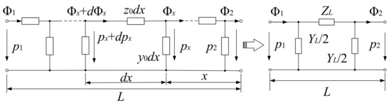
Figure 1.
The DPM of SP [27].
In this work, the DPM of SP is employed as an important part of the HP in a DHS. It is pointed out in [24] that the LP and radiator play important roles in an actual DHS, and have impacts on the performances of the IPHS and SP. Thus, the modeling of the LP and radiator will be carried out next to enhance DPM with reference to the existing differential analysis methods for DHS [14,22,23].
2.2. The LP Model and Radiator Model
In the DHS modeling and controlling presented in [24], the detailed models of LPs and radiator are addressed. Regretfully, these models are mainly transient state models and are hard to compute. In order to attain a simple steady state model, the typical dual-port network and three-port network are employed, as shown in Figure 2. In this work, four kinds of LP are included, i.e., the tee pipe, reducer union, elbow pipe, and valve. Based on a typical DHS, the formulas of the involved pressure resistances and thermal conductance in Figure 2 can be obtained.
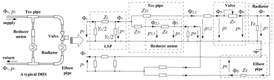
Figure 2.
The steady state model of a typical district heating system (DHS).
The detailed derivation procedures of some complicated equations are moved to Appendix A, so as to significantly simplify the presentation in the main body of the paper.
2.2.1. The Tee Pipe Model
In Figure 2, a typical three-port network is employed to describe the tee pipe. In [24], a detailed lumped parameter model for the tee pipe is presented, and the pressure resistances of the tee pipe can be attained by comparing the models in Figure 2 and [24].
where ZT1 and ZT2 are the pressure resistances of the two outlet pipes in the tee pipe, respectively; Kf is the local loss coefficient; dT and D1 are the inner diameter and inlet mass flow of the tee pipe, respectively; and, Φ2,1 and Φ2,2 respectively denote the heat flows at the two outlet pipes in the tee pipe.
2.2.2. The Reducer Union Model and Elbow Pipe Model
In Figure 2, a typical dual-port network is employed to depict the reducer union and the elbow pipe, respectively. By comparing the reducer union model and the elbow pipe model presented in [24], the pressure resistances of the reducer union ZR and elbow pipe ZE can be attained as
where D2,1 and D7 are, respectively, the inlet mass flows of the reducer union and elbow pipe; = (1 − dR12/dR22)2 denotes the local loss coefficient of the reducer union; dR1 and dE are the inlet inner diameters of the reducer union and elbow pipe, respectively; and, Φ3 and Φ8 are, respectively, the outlet heat flows of the reducer union and elbow pipe.
2.2.3. The Valve Model
In Figure 2, a variable resistor model is used to represent the valve. With reference to Equations (3)–(5) and some publications [28,29], the variable local loss coefficient Kf is presented here to formulate the variable pressure resistance of the valve ZV, as shown in Equations (6) and (7).
where D5 and Km ∈ [0, 1] are, respectively, the mass flow and the opening coefficient of the valve [29]; dV is the inlet inner diameter of the valve; and, α and β are both fitting coefficients. Φ6 is the outlet heat flow of the valve.
2.2.4. The Radiator Model
Due to the time coupling between temperature and heat transferring, the present radiator model is a differential equation [24,30]. This makes thermal analysis in a DHS very complicated. In order to rebuild a simpler model for the radiator, a two-terminal network is employed, as shown in Figure 2.
where Φ6, Φ7, ΦL, and YM denote the inlet heat, outlet heat, heat load, and thermal conductance of the radiator, respectively; p7 is the pressure of the radiator.
In Equation (8), the thermal conductance of the radiator is expressed by the discrete-time decoupled heat load ΦL, and thus makes the heat flow analysis much easier than the existing differential model for the radiator.
Based on the above stated three models, an equivalent simplified τ-type model can be attained, as detailed below.
2.3. Simplifications of the DHS Model
Despite the formulas that have been derived, the steady state model in Figure 2 is still computation-intensive, especially for the heat flow analysis. Therefore, some simplification is demanded to make the proposed model more tractable. Without loss of generality, a representative HP is employed to demonstrate the simplification process.
First, a representative HP is transformed into an equivalent τ-type steady state model, as shown in Figure 3.
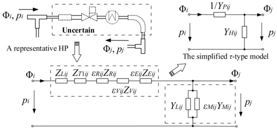
Figure 3.
The simplifications of the steady state model of a representative heating pipe (HP).
It is assumed that the composition of the representative HP is uncertain, because the composition is variable with the structure of HP. Then, the universal formulas of pressure conductance YPij and thermal conductance YHij can be attained as
where εRij, εVij, εEij, and εMij, respectively, denote the binary variables (1 or 0) that are indicating whether or not HP contains the reducer union, valve, elbow pipe, and radiator.
For any specific HP, the binary variables and other parameters in the above equations will become constants as long as its composition is specified. Therefore, the constants C1ij and C2ij could be used to simplify Equations (9) and (10), respectively. In next, ZLij and YLij in Equations (9) and (10) will be further expanded and simplified. More specifically, “sinh(•)” and “cosh(•)” in Equation (1) are expanded in Taylor’s series with the high order terms omitted. Thus, ZLij and YLij can be formulated as
where C3ij denotes the constant of the representative HP.
Then, YPij and YHij can be formulated as
where Cij denotes the constant of the representative HP.
Up to now, the simplified τ-type model of the representative HP is attained, as shown in Figure 3. The heat losses and pressure losses of HP can be formulated as Equations (15) and (16), respectively:
ΔΦij and Δpij can be calculated by the constants of the representative HP, i.e., C2ij, Cij, , c, and k, and the environment temperature T0. In other words, different pipeline parameters and temperatures will lead to different optimization strategies for a DHS regarding the coordinated planning and operation. Note that the heat flow and pressure distribution of a DHS decline during the process of hot water transferring, which, respectively, due to the heat transfer with the environment and the frictions of HPs. For the convenience of presentation, ΔΦij > 0 is used to describe the heat transferring process from hot water to environment, and Δpij > 0 represents pressure reduction. Note that the temperature of hot water is limited to be higher than T0 and the hot water is transferred without additional pressure, then ΔΦij and Δpij are both assumed to be non-negative numbers in this work.
3. The Optimal Heat-Power Flow Model
Based on the simplified τ-type model, a unified analysis method of heat and power flow in the IPHS will be addressed in this section.
3.1. The Connection Matrix of HP
Traditionally, the DHS adopts a loop structure and consists of two symmetric networks: the supply pipe network and the return pipe one [12]. Note that hot water is pressured by the circulating pump (CP) to the loop in a certain direction. To supply the heat demand, the hot water that is drained out of the CHP plant is transferred through the supply pipes network. After the heating process, hot water returns back to the CHP plant through the return pipes network. Hence, the mass flow of the HP can be assumed to be a non-negative number. The symmetric network means that more than one pipe connecting to the end of any HP in a DHS. Thus, the connection matrix of the HP becomes more crucial to simulate the distribution of heat flow and formulate the heat flow balance. In order to attain the connection matrix, an illustration, as shown in Figure 4, is employed:
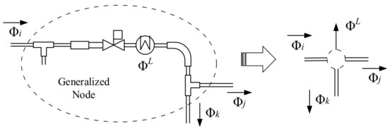
Figure 4.
Attainment of the HP connection matrix.
With respect to Figure 4, the connection matrix of the HP can be formulated as
where ξi,l donates an element of the HP connection matrix; ΩH is the set of nodes of the DHS; and, Φi, Φj and Φk, respectively, donate the inlet heat flow of HP i, HP j, and HP k.
It should be mentioned that the heat flow balance is established in the view of the HP rather than based on a DHS node. While hot water supplies heat demand by transferring through the radiator that is connected with a HP, this is significantly different from the situation of the power load that is connected at a specified bus point. To balance the heat flow, the HP is regarded as a generalized node, as shown in Figure 4. As to the pressure distribution, the analysis method is similar to the one that is used in voltage calculation for many years, i.e., the Distflow [31,32]. Referring to [31,32], it is known that the incidence matrix of the DHS is very vital to the analysis of the pressure distribution. The incidence matrix can be attained using the method that is presented in [33], and the details of the method will not be presented here due to the limited space.
3.2. The OHPF Model
Regarding the HP connection matrix, incidence matrixes, and generalized node, the OHPF model can be formulated mathematically. To coordinate different energy flows, the term “heat-power flow” is defined and employed in the OHPF model with the heat flow and power flow being uniformly modelled.
The presented OHPF model is a quadratic constrained optimization problem, as detailed below.
3.2.1. The Objective Function
The objective function of the OHPF model is defined as
3.2.2. The Constraints of DHS
The operation constraints of a DHS can be formulated as
3.2.3. The Constraints of PDS
The operation constraints of a PDS can be formulated as
3.2.4. The Constraints of Coupling Devices
The operation constraints of three kinds of coupling devices can be formulated as
where ΔOHPF means the optimization objective of the OHPF model; Γ is the run time of an IHPS; ΩL and ΩP are, respectively, the set of HPs in the DHS and the set of feeders in the PDS; ΔΦl and Δpl, respectively, denote the heat losses and the pressure losses of HP l; ΔPi, and ΔQi, respectively, denote the active and reactive power losses of feeder i; φH and φP, respectively, denote the unit price of heat power and that of electrical power; Φl is the inlet heat flow of HP l; pi is the pressure at node i; and Dl, respectively, denote the heat load and mass flow of HP l; Cl and C2l, respectively, denote the constants of HP l; , and respectively denote the thermal power output of the CHP plant, the thermal power output of the EB, and the pressure compensation of the CP in HP l; and are, respectively, the elements of the incidence matrixes of the DHS and PDS; and are, respectively, the upper and lower heat flow limits of HP l; and denote the upper and lower limits of the pressure at node i; Pi and Qi are, respectively, the active power and reactive power in feeder i; and respectively denote the injection active power and reactive power at the power-outflow terminal of feeder i; and are, respectively, the active and reactive loads at the power-outflow terminal of feeder i; , and respectively denote the power output of the CHP plant, the power demand of the CP, and the power demand of the EB at the power-outflow terminal of feeder i; CCHP is the heat-power ratio of the CHP plants; μCP is the efficiency factor of the CPs; CEB is the heat-power ratio of the EBs; and , respectively, denote the upper limits of active and reactive power in feeder i; Ri, Xi and ΔVi, respectively, denote the resistance, reactance, and voltage losses of feeder i; VB is the reference voltage of the PDS; Vi is the voltage at the power-outflow terminal of feeder i; and respectively denote the upper and lower limits of injection active power at the power-outflow terminal of feeder i; and denote the upper and lower limits of injection reactive power at the power-outflow terminal of feeder i; and respectively denote the upper and lower limits of the thermal power output of the CHP plant in HP l; and respectively denote the upper and lower limits of the pressure compensation of the CP in HP l; and denote the upper and lower limits of the power demand of the EB at the power-outflow terminal of feeder i; ΛEB, ΛCHP and ΛCP respectively denote the location transformation matrixes of the EBs, the CHP plants, and the CPs.
In the OHPF model, Equation (18) stands for the optimization objective function with heat losses and active power losses included; Equation (19) represents the heat losses and active power losses; Equation (20) represents active power balance and reactive power balance; Equation (21) represents pressure losses; Equation (22) denotes the mass flow balance; Equations (23) and (24), respectively, denote the upper and lower output limits of Dl, Φl and pi; Equation (25) represents the active power balance and reactive power balance; Equation (26) represents the constraints of Pi, Qi, and Vi; Equation (27) represents voltage losses; Equation (28) represents the constraints of injection active and reactive power; Equation (29) represents the models of CHP plants [34], CPs [27], and EBs [35], sequentially; Equation (30) includes the upper and lower output limits of CHP plants, CPs and EBs.
The well-established IPOPT (Interior Point OPTimizer) commercial solver based on YALMIP/MATLAB toolbox is employed to solve the developed quadratic OHPF model.
4. Case Studies
Two sample IPHS systems are served for demonstrating the feasibility of the proposed steady state model as well as the effects of the OHPF model in coordinated operation.
4.1. Sample System 1
The network of the first sample system (sample system 1) is shown in Figure 5, in which the CHP plants and CPs are employed as coupling devices between PDS and DHS.
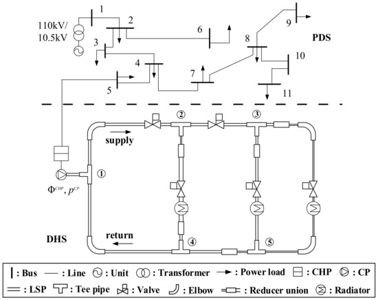
Figure 5.
The network of sample system 1.
4.1.1. Accuracy of the OHPF Model
The network structure and parameters of sample system 1 are all taken from [24]. Specified parameters are listed in Table 1.

Table 1.
Specified parameters of sample system 1.
In order to compare the results between heat-power flow and optimal heat-power flow, the upper and lower output limits of the coupling devices are first assumed to be the same and take the values specified in [24]. Since EBs are not addressed in [24], it is assumed that “ = = 0” and = = 0”. This means that and are constants and that they cannot be optimized. Thus, the heat flow and pressure distribution results that were attained by the OHPF model could be used to compare with those that are presented in [24], as shown in Figure 6.
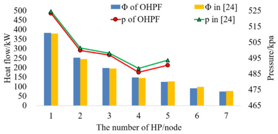
Figure 6.
The heat flow and pressure distribution of DHS in sample system 1.
From Figure 6, it can be found that the optimization results that were attained by the OHPF model are almost the same as those that are presented in [24]. This means that the accuracy of the OHPF model is acceptable, although some simplifications have been made to make the steady state model more tractable, as detailed in Section 2.
4.1.2. Temperature Sensitivity Analysis based on the OHPF Model
To investigate the effect of T0 on OHPF, three scenarios with different values of T0, i.e., −15 °C, −5 °C, and 5 °C, are examined. Equation (18) is formulated to minimize the heat losses and active power losses, with T0 remaining unchanged as long as the OHPF model can be successfully solved. That is because the outputs of the coupling devices could be adjusted in feasible regions to obtain the same minimum ΔΦ and ΔP, and hence the impacts of T0 can be waived. In order to analyze temperature sensitivity, it is specified that “φH = φP = 0” so as to prevent ΔΦ and ΔP from decreasing during the process of seeking the optimal solution of Equation (18). The optimal values of ΔΦ, Δp, D, ΔP, and voltage under different scenarios are attained, as shown in Table 2 and Figure 7.
Table 2.
ΔΦ, Δp, and D of DHS under different scenarios in sample system 1.
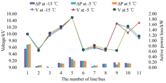
Figure 7.
ΔP and voltage of PDS in sample system 1.
In Table 2, ΔΦ decreases significantly with the increase of T0, and Δp maintains in step with ΔΦ. This is due to more drastic thermal interactions happening at low T0, which increases ΔΦ when hot water is transferred through a HP. Different levels of thermal interactions have impacts on Δp by decreasing the mass flow in the corresponding HP, but are not as significant as those on ΔΦ. When a lower T0 comes along with a higher output of the CHP plant, both in heat and power, different levels of ΔP and voltage of PDS will occur, as shown in Figure 7. In summary, the state variables of the OHPF model, i.e., ΔΦ, Δp, D, ΔP and voltage, are all sensitive to T0.
4.2. Sample System 2
Based on the mentioned methods, a software package named “Multi-Flow” is developed to online attain the coordinated optimal operation strategy for any IPHS, as shown in Figure 8. In “Multi-Flow”, the OHPF model is coded in MATLAB, and its reliability and efficiency are tested by numerous sample systems. Once an IPHS is built up by component modules, optimal heat-power flow can then be carried out. The involved parameters are included in the menu-bar for setting different simulation scenarios. MATLAB and YALMIP toolboxes are employed to provide computing services for “Multi-Flow”.
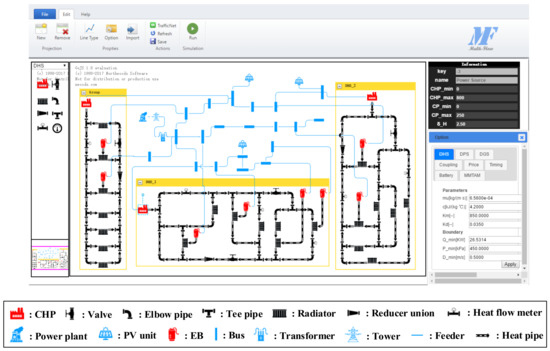
Figure 8.
The network of sample system 2 attained by the software “Multi-Flow”.
In sample system 2, a larger IPHS is built based on the software “Multi-Flow” that was developed by us. Three DHSs are integrated into a PDS with three photovoltaic (PV) generating units being included. The impacts of electric heating on the accommodation capability for PV generation are examined for three different load-level scenarios. The daily power and heat loads of sample system 2 are given in Figure A1 and Figure A2 of Appendix B.
To demonstrate the impacts of different load levels on OHPF, Φ and voltage at different time points, i.e., 5:00, 13:00, and 21:00, are calculated and are shown in Figure 9. The values of φH and φP are specified to be 0, as what has been done in sample system 1. Simulation results show that Φ of DHS and the voltage of PDS are both different under various load levels. Specifically, the higher levels of heat and power loads at 13:00 lead to lower heat flow and smaller voltage fluctuation. This is because a higher heat demand will increase the heat outputs of CHP plants. As a result, the power outputs from CHP plants increase significantly to support the power demand and improve the voltage distribution.
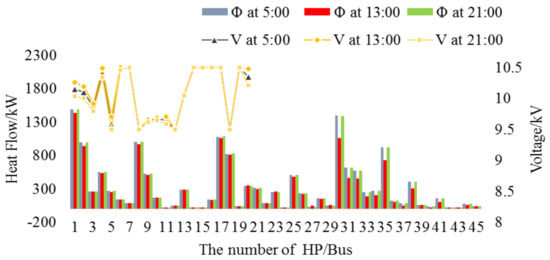
Figure 9.
Heat flows and pressure distributions at different time points.
As shown in Figure 8, EBs can be employed to enhance the accommodating capability for PV power generation. The hourly PV power outputs in a day are shown in Figure A3 of Appendix B. To attain the optimal operation strategy for sample system 2, Equation (18) is employed to minimize the operational costs. Moreover, in order to maintain the optimization objective of Equation (18) as unchanged, electricity purchasing costs are not considered, and the punishment costs for PV generation curtailment are not included as well. Then, the following three scenarios with different ratios of the electric load over the heating load are examined to find out the impacts of EBs on the optimal operation strategy:
- (1)
- S1: No electric heating load;
- (2)
- S2: 50% of the heating load is supplied by EBs; and,
- (3)
- S3: The heating load is fully supplied by EBs.
The power outputs of PV units and CHP plants under these three scenarios are attained by the presented OHPF model, as shown in Figure 10.
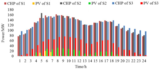
Figure 10.
The power outputs of photovoltaic (PV) units and combined heat and power (CHP) plants under three scenarios.
From Figure 10, it is obvious that the power outputs from the PV units increase with the raise of the electric-heating ratio. The power outputs of the PV units under these three scenarios are shown in Figure A3 of Appendix B. The reduced demand of hot water led to a declined thermal power output of the CHP plant. As a result, the heating flow through the DHS reduced, and the heating losses also reduced accordingly. In a nutshell, electric heating makes contributions to the economic operation of a DHS and the accommodation capability enhancement of PV power generation.
Regarding a PDS, heating with EBs could increase the power load demand, and will have impacts on the PDS planning process. In analyzing the economics of EBs, the costs for expansion planning and operation should be taken into account. In-depth study will be carried out in the future to figure out the economics of employing EBs and the coordinated planning for an IHPS.
5. Conclusions
A steady state model for an IPHS is presented in this work, with the impacts of pipeline parameters and environment temperature being taken into account. In the presented model, various components of HP are modeled, and the hydraulic sub-model is combined with the thermal one. Then, an OHPF model is proposed to analyze the performance of an IPHS. Two sample systems are served for demonstrating the proposed method. It is shown by the simulation results that the accuracy of the presented OHPF model is acceptable and the optimization results of the OHPF model are sensitive to environment temperature. The optimal operation strategies that are attained by the OHPF model are demonstrated with three scenarios under different load levels. The electric heating load makes contributions to the economic operation of a DHS and the accommodation of PV power generation.
The following issues will be carried out in the future:
- (1)
- The OHPF model will be employed to optimize the coordinated planning and the operation strategies for integrated heat-gas-power energy systems by including the operation constraints of the nature gas distribution system.
- (2)
- Modeling of heat storage equipment will be addressed to expand the steady state model that is presented in this work, and to include more feasible operation modes of IPHSs.
- (3)
- Intelligent traffic networks with various kinds of electric vehicles will be included in the expansion planning of multi-energy systems and charging infrastructures.
Acknowledgments
This work is jointly supported by The National Key Research and Development Program of China (Basic Research Class) (No. 2017YFB0903000), the National Natural Science Foundation of China (No. U1509218), and the Science and Technology Project of Guangzhou Power Supply Company Limited (No. GZHKJXM20160034).
Author Contributions
Wentao Yang proposed the methodological framework and mathematical model, performed simulations and drafted the manuscript; Fushuan Wen organized the research team, reviewed and improved the methodological framework and implementation algorithm; Ke Wang and Yuchun Huang reviewed the manuscript and provided suggestions; Md. Abdus Salam reviewed and polished the manuscript. All authors discussed the simulation results and agreed for submission.
Conflicts of Interest
The authors declare no conflict of interest.
Nomenclatures
| PDS | Power distribution system |
| DHS | District heating system |
| OHPF | Optimal heat-power flow |
| CHP | Combined heat and power |
| EBs | Electric boilers |
| IPHS | Integrated power and heating systems |
| HP | Heating pipe |
| SP | Straight pipe |
| LP | Local pipe |
| DPM | Distributed parameter model |
| CP | Circulating pump |
| PV | Photovoltaic |
| ZL | Equivalent pressure resistance of SP [kpa/kW] |
| YL | Equivalent thermal conductance of SP [kW/kpa] |
| Φ | Inlet or outlet heat flow of a HP [kW] |
| p | Pressure of a HP [kpa] |
| D | Mass flow of a HP [kg/s] |
| dL | Inner diameter of SP [m] |
| λ | Friction factor of SP |
| L | Length of SP [m] |
| ρ | Density of hot water [t/m3] |
| c | Specific heat of hot water [kJ/(kg·K)] |
| k | Heat transferring coefficient of the pipe wall [W/(m·K)] |
| T0 | Environment temperature [°C] |
| z0 | Unit pressure resistance of SP [kpa/kW] |
| y0 | Unit thermal conductance of SP [kW/kpa] |
| ZT | Pressure resistances of outlet pipe in the tee pipe [kpa/kW] |
| Kf | Local loss coefficient |
| dT | Inner diameter of the tee pipe [m] |
| Local loss coefficient of the reducer union | |
| ZR | Pressure resistances of the reducer union [kpa/kW] |
| ZE | Pressure resistances of the elbow pipe [kpa/kW] |
| dR1 | Inner diameter of the reducer union [m] |
| dE | Inner diameter of the elbow pipe [m] |
| ZV | Variable pressure resistance of the valve [kpa/kW] |
| dV | Inlet inner diameter of the valve [m] |
| α, β | Fitting coefficient of the valve |
| ΦL | Heat load [kW] |
| YM | Thermal conductance of the radiator [kW/kpa] |
| εRij | Binary variables that indicating whether or not HP contains the reducer union |
| εVij | Binary variables that indicating whether or not HP contains the valve |
| εEij | Binary variables that indicating whether or not HP contains the elbow pipe |
| εMij | Binary variables that indicating whether or not HP contains the radiator |
| C1ij, C2ij, C3ij, Cij | Constants of the representative HP |
| ξi,l | An element of the HP connection matrix |
| ΩH | Set of nodes of the DHS |
| ΔOHPF | Optimization objective of the OHPF model [104 $] |
| Γ | Run time of an IHPS [h] |
| ΩL | Set of HPs in the DHS |
| ΩP | Set of feeders in the PDS |
| ΔΦl | Heat losses of HP l [kW] |
| Δpl | Pressure losses of HP l [kpa] |
| ΔPi | Active power losses of feeder i [MW] |
| ΔQi | Reactive power losses of feeder i [MVar] |
| φH | Unit price of heat power [$/(MW·h)] |
| φP | Unit price of electrical power [$/(MW·h)] |
| Thermal power output of the CHP plant in HP l [kW] | |
| Thermal power output of the EB in HP l [kW] | |
| Pressure compensation of the CP in HP l [kpa] | |
| Elements of the incidence matrixes of the DHS | |
| Elements of the incidence matrixes of the PDS | |
| Upper and heat flow limit of HP l [kW] | |
| Lower heat flow limit of HP l [kW] | |
| Upper limit of the pressure at node i [kpa] | |
| Lower limit of the pressure at node i [kpa] | |
| Pi | Active power in feeder i [MW] |
| Qi | Reactive power in feeder i [MVar] |
| Upper limit of active power in feeder i [MW] | |
| Upper limit of reactive power in feeder i [MVar] | |
| Injection active power at the power-outflow terminal of feeder i [MW] | |
| Injection reactive power at the power-outflow terminal of feeder i [MVar] | |
| Active loads at the power-outflow terminal of feeder i [MW] | |
| Reactive loads at the power-outflow terminal of feeder i [MVar] | |
| Power output of the CHP plant at the power-outflow terminal of feeder i [MW] | |
| Power demand of the CP at the power-outflow terminal of feeder i [MW] | |
| Power demand of the EB at the power-outflow terminal of feeder i [MW] | |
| CCHP | Heat-power ratio of the CHP plants |
| μCP | Efficiency factor of the CPs [kpa/MW] |
| CEB | Heat-power ratio of the EBs |
| Pi | Upper limit of active power in feeder i [MW] |
| Qi | Upper limit of reactive power in feeder i [MVar] |
| Ri | Resistance of feeder i [Ω/km] |
| Xi | Reactance of feeder i [Ω/km] |
| ΔVi | Voltage losses of feeder i [kV] |
| VB | Reference voltage of the PDS [kV] |
| Vi | Voltage at the power-outflow terminal of feeder i [kV] |
| Upper limit of injection active power at the power-outflow terminal of feeder i [MW] | |
| Lower limit of injection active power at the power-outflow terminal of feeder i [MW] | |
| Upper limit of injection reactive power at the power-outflow terminal of feeder i [MVar] | |
| Lower limit of injection reactive power at the power-outflow terminal of feeder i [MVar] | |
| Upper limit of the thermal power output of the CHP plant in HP l [kW] | |
| Lower limit of the thermal power output of the CHP plant in HP l [kW] | |
| Upper limit of the pressure compensation of the CP in HP l [kpa] | |
| Lower limit of the pressure compensation of the CP in HP l [kpa] | |
| Upper limit of the power demand of the EB at the power-outflow terminal of feeder i [MW] | |
| Lower limit of the power demand of the EB at the power-outflow terminal of feeder i [MW] | |
| ΛEB | Location transformation matrixes of the EBs |
| ΛCHP | Location transformation matrixes of the CHP plants |
| ΛCP | Location transformation matrixes of the CPs |
Appendix A
Appendix A.1. The Tee Pipe Model
In Figure 2, a typical three-port network is employed to describe the tee pipe and can be formulated as Equation (A1).
where Φ1 and p1 are respectively the inlet heat flow and pressure of the tee pipe; Φ2,1 and Φ2,2 respectively denote the heat flows at the two outlet pipes in the tee pipe; p2,1 and p2,2 are respectively the pressures of the two outlet pipes in the tee pipe; ZT1 and ZT2 are respectively the pressure resistances of the two outlet pipes in the tee pipe.
The tee pipe model in [24] can be expressed as
where Kf is the local loss coefficient; dT is the inner diameter of the inlet pipe; D1, D2,1 and D2,2 denote the mass flows of different pipes, respectively; H1, H2,1 and H2,2 denote the enthalpies of different pipes, respectively.
“DH” in Equation (A2) can be replaced by “Φ” since “Φ = DH” [4]. Then, ZT1 and ZT2 can be attained by comparing Equation (A2) with Equation (A1).
Appendix A.2. The Reducer Union Model and Elbow Pipe Model
In Figure 2, a typical dual-port network is employed to depict the reducer union and the elbow pipe respectively, and formulated as
where Φ2,1 and p2,1 are respectively the inlet heat flow and pressure of the reducer union; Φ3 and p3 are respectively the outlet heat flow and the pressure of the reducer union; Φ7 and p7 are respectively the inlet heat flow and the pressure of the elbow pipe; Φ8 and p8 are respectively the outlet heat flow and pressure of the elbow pipe; ZR and ZE are the pressure resistances of the reducer union and elbow pipe, respectively.
By comparing the reducer union model and elbow pipe model presented in [24] (Equations (A6) and (A7)), ZR and ZE can be attained as
where D2,1 and H2,1 are respectively the inlet mass flow and enthalpy of the reducer union; D3 and H3 are respectively the outlet mass flow and enthalpy of the reducer union; = (1 − dR12/dR22)2 denotes the local loss coefficient of the reducer union; dR1 and dR2 are the inlet inner diameter and outlet inner diameter of the reducer union, respectively; dE, D7 and H7 are the inlet inner diameter, mass flow and enthalpy of the elbow pipe, respectively; D8 and H8 are respectively the outlet mass flow and the enthalpy of the elbow pipe.
Appendix A.3. The Valve Model
In Figure 2, a variable resistor model, as detailed below, is used to represent the valve:
where Φ5 and p5 are respectively the inlet heat flow and the pressure of the valve; Φ6 and p6 are respectively the outlet heat flow and the pressure of the valve; ZV is the variable pressure resistance of the valve.
With reference to Equations (A8) and (A9) and other publications [28,29], the variable local loss coefficient Kf is presented here to formulate ZV, as shown in Equations (A11) and (A12).
where D5 and Km ∈ [0, 1] are respectively the mass flow and opening coefficient of the valve [29]; dV is the inlet inner diameter of the valve; α and β are both fitting coefficients.
Appendix B
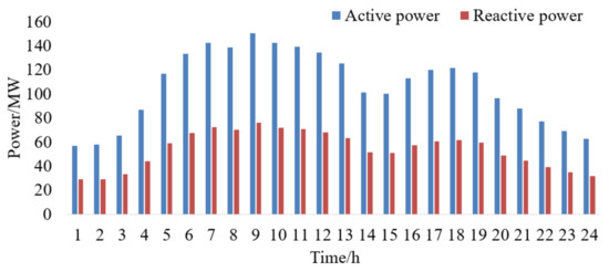
Figure A1.
Daily active and reactive loads in sample system 2.
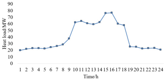
Figure A2.
Daily heating loads in sample system 2.
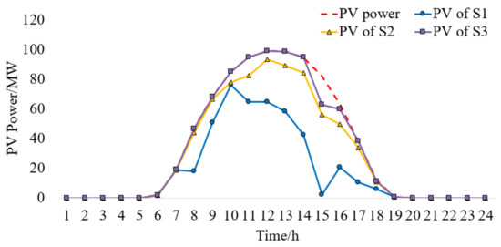
Figure A3.
The power outputs of PV units under different scenarios in sample system 2.
References
- Chen, Y.; Liu, Y.; Hung, S.; Cheng, C. Multi-input inverter for grid-connected hybrid PV/wind power system. IEEE Trans. Power Electron. 2007, 22, 1070–1077. [Google Scholar] [CrossRef]
- Momete, D.C. Measuring renewable energy development in the Eastern Bloc of the European Union. Energies 2017, 10, 2120. [Google Scholar] [CrossRef]
- Raunbak, M.; Zeyer, T.; Zhu, K.; Greiner, M. Principal mismatch patterns across a simplified highly renewable European electricity network. Energies 2017, 10, 1934. [Google Scholar] [CrossRef]
- Gu, Z.; Kang, C.; Chen, X.; Bai, J.; Cheng, L. Operation optimization of integrated power and heat energy systems and the benefit on wind power accommodation considering heating network constraints. Proc. CSEE 2015, 35, 3596–3604. [Google Scholar]
- Wang, J.; Gu, W.; Lu, S.; Zhang, C.; Wang, Z.; Tang, Y. Coordinated planning of multi-district integrated energy system combining heating network model. Autom. Electric Power Syst. 2016, 40, 17–24. [Google Scholar]
- Jia, C.; Wu, C.; Zhang, C.; Zhou, J.; Liu, G.; Bai, M.; Cai, Y.; Tang, W.; Sun, C. Optimum configuration of energy station in urban hybrid area of commerce and residence based on integrated planning of electricity and heat system. Power Syst. Prot. Control 2017, 45, 30–36. [Google Scholar]
- Bakken, B.H.; Dyken, S.V. Integrated planning of electricity, gas and heat supply to municipality. Strojarstvo 2013, 55, 109–126. [Google Scholar]
- Li, J.; Fang, J.; Zeng, Q.; Chen, Z. Optimal operation of the integrated electrical and heating systems to accommodate the intermittent renewable sources. Appl. Energy 2016, 167, 244–254. [Google Scholar] [CrossRef]
- Lyu, Q.; Jiang, H.; Chen, T.; Wang, H.; Lyu, Y. Wind power accommodation by combined heat and power plant with electric boiler and its national economic evaluation. Autom. Electric Power Syst. 2014, 38, 6–12. [Google Scholar]
- Chen, J.; Wu, W.; Zhang, B.; Sun, Y. A rolling generation dispatch strategy for co-generation units accommodating large-scale wind power integration. Autom. Electric Power Syst. 2012, 36, 21–27. [Google Scholar]
- Chen, X.; Kang, C.; O’Malley, M.; Xia, Q.; Bai, J. Increasing the flexibility of combined heat and power for wind power integration in China: Modeling and implications. IEEE Trans. Power Syst. 2015, 30, 1848–1857. [Google Scholar] [CrossRef]
- Jing, Z.; Jiang, X.; Wu, Q.; Tang, W.; Hua, B. Modelling and optimal operation of a small-scale integrated energy based district heating and cooling system. Energy 2014, 73, 399–415. [Google Scholar] [CrossRef]
- Shabanpour-Haghighi, A.; Seifi, A.R. Simultaneous integrated optimal energy flow of electricity, gas, and heat. Energy Convers. Manag. 2015, 101, 579–591. [Google Scholar] [CrossRef]
- Cahill, D.G. Analysis of heat flow in layered structures for time-domain thermoreflectance. Rev. Sci. Instrum. 2004, 75, 5119–5122. [Google Scholar] [CrossRef]
- Liu, X.; Wu, J.; Jenkins, N.; Bagdanavicius, A. Combined analysis of electricity and heat networks. Appl. Energy 2016, 162, 1238–1250. [Google Scholar] [CrossRef]
- Gamberi, M.; Manzini, R.; Regattieri, A. Simulink©, simulator for building hydronic heating systems using the Newton-Raphson algorithm. Energy Build. 2009, 41, 848–855. [Google Scholar] [CrossRef]
- Fedorov, M. Parallel implementation of a steady state thermal and hydraulic analysis of pipe networks in OpenMP. Lect. Notes Comput. Sci. 2009, 17, 360–369. [Google Scholar]
- Kona, A.; Verda, V. Multiobjective optimization applied to district heating network planning. Compet. Intell. Rev. 2011, 5, 64–66. [Google Scholar]
- Wang, H.; Duanmu, L.; Li, X.; Lahdelma, R. Optimizing the district heating primary network from the perspective of economic-specific pressure loss. Energies 2017, 10, 1095. [Google Scholar] [CrossRef]
- Aringhieri, R.; Malucelli, F. Optimal operations management and network planning of a district heating system with a combined heat and power plant. Ann. Oper. Res. 2003, 120, 173–199. [Google Scholar] [CrossRef]
- Obara, S.; Kudo, K. Route planning and estimate of heat loss of hot water transportation piping for fuel cell local energy network. Trans. Jpn. Soc. Refrig. Air Cond. Eng. 2005, 22, 13–24. [Google Scholar]
- Zhang, S.; Jin, Z.; Hao, L.; Wang, X.; Chen, P. An analysis on the safety performance of the combined fittings of straight tees and long radius elbows. Chem. Eng. Mach. 2008, 4, 151–158. [Google Scholar]
- Xu, B.; Fu, L.; Di, H. Dynamic simulation of space heating systems with radiators controlled by TRVs in buildings. Energy Build. 2008, 40, 1755–1764. [Google Scholar] [CrossRef]
- Wang, Y. Research of Modeling and Control Method for District Heating System; Southeast University: Nanjing, China, 2013; pp. 18–44. [Google Scholar]
- Liu, X.; Mancarella, P. Modelling, assessment and Sankey diagrams of integrated electricity-heat-gas networks in multi-vector district energy systems. Appl. Energy 2016, 167, 336–352. [Google Scholar] [CrossRef]
- Geidl, M.; Andersson, G. Optimal power flow of multiple energy carriers. IEEE Trans. Power Syst. 2007, 22, 145–155. [Google Scholar] [CrossRef]
- Xu, Y.; Yang, W.; Qi, F.; Wen, F.; Zhao, J.; Dong, Z. A distributed parameter model of heating pipe networks and coordinated planning of electrical and heating coupled systems. Electric Power Constr. 2017, 38, 77–87. [Google Scholar]
- Chen, Q.; Fu, R.; Xu, Y. Electrical circuit analogy for heat transfer analysis and optimization in heat exchanger networks. Appl. Energy 2015, 139, 81–92. [Google Scholar] [CrossRef]
- Bojic, M.; Trifunovic, N. Linear programming optimization of heat distribution in a district-heating system by valve adjustments and substation retrofit. Build. Environ. 2000, 35, 151–159. [Google Scholar] [CrossRef]
- Chotivisarut, N.; Kiatsiriroat, T. Cooling load reduction of building by seasonal nocturnal cooling water from thermosyphon heat pipe radiator. Int. J. Energy Res. 2010, 33, 1089–1098. [Google Scholar] [CrossRef]
- Yeh, H.G.; Gayme, D.F.; Low, S.H. Adaptive VAR control for distribution circuits with photovoltaic generators. IEEE Trans. Power Syst. 2012, 27, 1656–1663. [Google Scholar] [CrossRef]
- Faqiry, M.N.; Edmonds, L.; Zhang, H.; Khodaei, A.; Wu, H. Transactive-market-based operation of distributed electrical energy storage with grid constraints. Energies 2017, 10, 1891. [Google Scholar] [CrossRef]
- Marguc, J.; Truntic, M.; Rodic, M.; Milanovic, M. Modelling of power electronics converters by using the incidence matrix approach. In Proceedings of the IEEE International Symposium on Industrial Electronics, Edinburgh, UK, 19–21 June 2017; pp. 1–6. [Google Scholar]
- Zafra-Cabeza, A.; Ridao, M.A.; Alvarado, I.; Camacho, E.F. Applying risk management to combined heat and power plants. IEEE Trans. Power Syst. 2008, 23, 938–945. [Google Scholar] [CrossRef]
- Liao, Z.; Dexter, A.L. The potential for energy saving in heating systems through improving boiler controls. Energy Build. 2004, 36, 261–271. [Google Scholar] [CrossRef]
© 2018 by the authors. Licensee MDPI, Basel, Switzerland. This article is an open access article distributed under the terms and conditions of the Creative Commons Attribution (CC BY) license (http://creativecommons.org/licenses/by/4.0/).