Article

Robust Building Energy Load Forecasting Using Physically-Based Kernel Models

1
Energy Science, Technology and Policy, Carnegie Mellon University, Pittsburgh, PA 15213, USA
2
Department of Civil and Environmental Engineering, Carnegie Mellon University, Pittsburgh, PA 15213, USA
3
Department of Civil and Environmental Engineering, Stanford University, Stanford, CA 94305, USA
*
Author to whom correspondence should be addressed.
Current address: Carnegie Mellon University, 5000 Forbes Avenue, Pittsburgh, PA 15213, USA.
Energies 2018, 11(4), 862; https://doi.org/10.3390/en11040862
Submission received: 1 February 2018 / Revised: 31 March 2018 / Accepted: 4 April 2018 / Published: 8 April 2018
(This article belongs to the Special Issue Bayesian Building Energy Modeling)

Abstract

:
Robust and accurate building energy load forecasting is important for helping building managers and utilities to plan, budget, and strategize energy resources in advance. With recent prevalent adoption of smart-meters in buildings, a significant amount of building energy consumption data became available. Many studies have developed physics-based white box models and data-driven black box models to predict building energy consumption; however, they require extensive prior knowledge about building system, need a large set of training data, or lack robustness to different forecasting scenarios. In this paper, we introduce a new building energy forecasting method based on Gaussian Process Regression (GPR) that incorporates physical insights about load data characteristics to improve accuracy while reducing training requirements. The GPR is a non-parametric regression method that models the data as a joint Gaussian distribution with mean and covariance functions and forecast using the Bayesian updating. We model the covariance function of the GPR to reflect the data patterns in different forecasting horizon scenarios, as prior knowledge. Our method takes advantage of the modeling flexibility and computational efficiency of the GPR while benefiting from the physical insights to further improve the training efficiency and accuracy. We evaluate our method with three field datasets from two university campuses (Carnegie Mellon University and Stanford University) for both short- and long-term load forecasting. The results show that our method performs more accurately, especially when the training dataset is small, compared to other state-of-the-art forecasting models (up to 2.95 times smaller prediction error).

1. Introduction

Governments across the world and private corporations are running a wide array of programs and initiatives for reducing energy consumption and improving energy efficiency in the energy consuming, transmitting and generating systems [1,2,3]. Among many sectors that consume energy, buildings take about 40% of the US’s total energy consumption and 20% of the world’s total energy consumption, according to the United States Energy Information Administration [4,5]. The first step towards reducing energy consumption and improving energy efficiency is to accurately predict how much energy will be consumed and what the associated uncertainties are. This will enable utilities and building energy managers to plan the energy budget accordingly. In addition, load forecasting has become increasingly important recently due to the increasing penetration of renewable energy [6,7].
Work on modeling energy consumption and predicting the future energy demand already exists. These works can be broadly classified into physics-based white box modeling and data-driven black box modeling of the energy consumption of a building [8]. White box models mainly include using building energy simulation software such as eQuest [9], EnergyPlus [10], etc. For example, EnergyPlus, which is a United States Department of Energy tool, can be used to model and simulate a building space and can output energy consumption, thermal comfort and other parameters of the building based on different inputs. These models can provide accurate results provided that there are similarly accurate and specific inputs [11,12,13,14,15], such as construction aspects of the building, heating and cooling system characteristics, appliance operating schedules etc., which are often difficult to obtain in practice. Recently, data-driven models, both deterministic and probabilistic have also been widely adopted [16,17,18,19,20] as large amounts of data have been made available to building owners, energy managers and utilities with the influx of smart-meters and other monitoring equipment [21,22,23,24]. However, these models require large amounts of training data for accurate predictions.
Hence, this paper introduces a new energy forecasting method, based on Gaussian Process Regression (GPR) that utilizes only two physical parameters, that is (1) the time of day and (2) the external temperature and other heuristics on energy consumption patterns to improve accuracy and robustness of load prediction while reducing the need for extensive training data or prior knowledge. This is due to the advantages of the GPR: modeling flexibility due to its non-parametric nature and computational efficiency for both load forecasting and uncertainty quantification through Bayesian updating. Exploiting these advantages, initial research work has been conducted for applying GPR to load forecasting, showing promising results [25,26,27,28,29]. However, further investigation and development are necessary to facilitate practical application of the method in this field, such as minimal requirement for training, robustness to diverse forecasting scenarios (prediction horizon, load type, aggregation level, etc.), and field validation across these scenarios.
To this end, this paper makes three main contributions: (1) The paper introduces a data-driven GPR-based method that incorporates just two physical parameters, namely time of day and external temperature (for training) and other heuristics about the load data to accurately forecast a building’s energy load with minimum training data (2) It investigates the characteristics of energy consumption data for different prediction horizon scenarios, which are used for covariance function modeling to improve the robustness of load forecasting algorithm; and (3) The load forecasting performance of our method is evaluated with field datasets collected from real campus buildings under diverse forecasting scenarios, including consumption type, size of training data, prediction horizon, and energy aggregation level.
For evaluation, we tested our methods with three field datasets collected from Stanford University and Carnegie Mellon University campus buildings for both short-term (10 min ahead) and long-term (1–5 day ahead) prediction of different types of building energy loads: lighting, Heating Ventilation and Air Conditioning (HVAC), and plug loads.
The rest of the paper is organized as follows. In Section 2, a review of the existing literature on load forecasting methods is provided. Section 3 discusses in detail about our forecasting approach using Gaussian Processes (GPR) and the kernel design for the covariance function of the GPR. We discuss the experimental setup and the results in Section 4. Finally, Section 5 provide conclusions.

2. Related Work

As mentioned in the previous section, building energy load forecasting can be achieved by physics-based white box models and data-driven black box models. Due to the complexity of building system, white box models often involves sophisticated simulation tools [11,12,13,14,15,30]. In [30], the authors have used EnergyPlus and used several input parameters such as the type of internal loads (lighting, computers etc.), their schedules, maximum and minimum dry-bulb temperature, and wind speed and direction. Some of these parameters are difficult to obtain as they have mentioned in the paper that they had to conduct several inspections to obtain these and even then, they needed to make assumptions about the occupancy profile for the building. Their simulated model had a prediction error rate of around 13%. Similarly, in [31], authors have used four different simulation tools and compared their performances. They used Energy10 [32], Green Building Studio, eQuest and EnergyPlus for simulation and they required very detailed building structure inputs: U-value of the roofs, walls, windows and load and space conditions (temperature set points of the HVAC systems, number of people) and HVAC design type. Similarly, refs. [11,12,13] have used EnergyPlus and [14,15] have used eQuest tools for obtaining energy forecasts for buildings.Simulation tools can provide accurate results [11,12,13,14,15,31], but they need information regarding the building infrastructure and operating patterns, which might be hard to obtain [33].
Data-driven black box models for load forecasting involve machine learning algorithms for regression. Both deterministic models, such as Neural Networks, Support Vector Regression (SVR), and Autoregressive Integrated Moving Average (ARIMA) models, and probabilistic models such as Bayesian Networks, Random Forests etc. have been developed for forecasting the consumption of different types of buildings—residential, commercial etc. and with different input features—temperature, occupancy, weather parameters etc. [34,35,36,37,38,39,40,41,42]. These models eliminate the need for extensive prior knowledge about the buildings and users; however, they often require a large amount of training data for each building of interest [34,35,36,39] or result in insufficient prediction accuracy, especially for long-term forecasting (1–5 day ahead forecasting) [37,40,43,44]. Among many, neural networks have been widely used in load forecasting [18,19,29,34,36,37] to obtain accurate predictions of building loads. Neural Network models take different inputs such as environmental parameters, occupancy information, inputs from the sensors on the HVAC system etc. to provide accurate load forecasts [34,35,37]. However, neural networks require significant amount of training data to produce such accurate results [34,36] and hence are not always suited for building load prediction, particularly in newly constructed buildings, where there is not much historical data available. Other algorithms, such as Support Vector Regression [18,19,38,39,43,45], Random Forests [41,42] and Autoregressive models [44,46] have also been used to develop models for building load prediction. They have been used for commercial building load forecasting and for short-term and day-ahead load predictions. Similar to neural networks, these methods do not require any prior knowledge but overcomes that requirement using significant periods of historical training data to produce accurate results [39,41,43,44,46]. In addition, AR models may not perform well in cases where there are high variations in the data [47,48,49].
To incorporate a systematic way to model and process data in probabilistic way, Bayesian methods, such as Bayesian Networks and Gaussian Processes have also been employed for load forecasting in buildings [25,27,40,50,51,52,53,54]. Bayesian Network approaches construct network graphs to represent how various inputs impact building’s energy loading [40,50,51,52]. However, this model also suffers from either extensive training or low accuracy (reported prediction error around 15–20%). Gaussian Process Regression (GPR) has been used in various fields including image-processing [54,55], robotics [56,57,58], people tracking [59], MRI scan analysis [60,61,62], etc. for regression and prediction by modeling the overall structure of the data as a joint Gaussian distribution and characterizing them using by modeling various kernel functions in the covariance matrix [63]. GPR has also been used for predicting various energy loads, including peak energy demand, short-term power output from photo-voltaic cells, machine energy usage prediction, utility level load forecasting, and short term load forecasting [26,27,28,29,53,64]. These studies show that GPR has been successfully used for forecasting energy loads and provide promising results for the predictions. However, to enable robust application of GPR for load forecasting in practice, further studies are necessary to develop methods to model GPR for different forecasting scenarios and validate with field datasets in diverse settings. This paper will investigate the characteristics of building energy loads of different types in different prediction horizon and incorporate this knowledge for modeling covariance function of GPR as described in Section 3 and evaluate with multiple field dataset in Section 4.

3. Building Energy Load Forecasting Algorithm Using Gaussian Process

Our load forecasting method models building energy consumption data such as a Gaussian Process ( G P ) and predict short- and long-term energy demand using the Bayes’ rule. The key component of the G P modeling involves learning the covariance function among the output data (e.g., energy demand) in terms of other input data (e.g., temperature, time of the day, etc.). In other words, the covariance function of the G P represents the underlying structure/relationship of the output data in terms of the input data. In our method, we first investigate the characteristics of energy load data in different scenarios (prediction horizon, type of load) to model the covariance function accordingly. Various kernels are used to incorporate the observed data characteristics. We will describe G P in detail in Section 3.1 and explain the covariance function modeling in Section 3.2. Our method is evaluated with field datasets, and the results are presented in Section 4.

3.1. Gaussian Process Regression

A Gaussian process ( G P ) is a stochastic process that is a collection of random variables, any finite number of which follow a joint Gaussian distribution. Just as probability distributions describe the likeliness of random variables which are scalars or vectors (for multivariate distributions), a stochastic process governs the properties and likeliness of functions, f ( x ) . In such a setting, a Gaussian Process is a non-parametric generalization of the Gaussian probability distribution. This is because a G P can model any finite number of function output, and thus the dimension of its parameters can grow to any number as more output data are observed [63].
This is very useful, as it provides much greater flexibility to model the data in any form. For example, in linear regression, if we assume a dependent variable y can be modeled as a function of an independent random variable x, that is: y = f ( x ) + ϵ , then this produces accurate results only when the function f defines a linear relationship ( f ( x ) = θ 0 + θ 1 x ). Learning the linear regression model tries to find the parameters θ 0 and θ 1 that best fits the observed data for x and y. As G P does not limit the model to any particular number of parameters, it finds a distribution over all possible functions that are consistent with the observed data.
Just like a Gaussian distribution, a G P is defined by a mean function, m ( x ) , and a covariance function, k ( x , x ) ,
f ( x ) GP ( m ( x ) , k ( x , x ) )
where
m ( x ) = E [ f ( x ) ]
k ( x , x ) = E [ ( f ( x ) m ( x ) ) ( f ( x ) m ( x ) ) ]
Usually, a prior mean function can be a constant or a simple function with a polynomial form of one or two degree. Using such a prior mean function is not restrictive as the posterior will be computed based on the data (i.e., the functional form of the mean function will be updated according to the training data patter after updating).
The properties of the function f ( x ) to be considered in the regression are incorporated into the G P model mostly through the covariance function. The covariance function encodes the assumptions about the function outputs in terms of x that are to be learned. For example, particular families of covariance functions can be chosen in order to emphasize the smoothness or the periodicity in the functions. For such functions, the degree of change and stationarity can be fine-tuned by setting its parameters, called hyper-parameters. We can also define other characteristics such as sudden spikes or periodicity in the functions, as described in Section 3.2. Therefore, obtaining the best covariance function is the goal of training a GPR model. As can be seen in Section 3.2, we can select a family or a combination of families of covariance functions and set hyper-parameters based on the characteristics of the observations.
Note that in Equation (1), even though the mean and the covariance functions are properties of function outputs f ( x ) , they are defined by input values x. The outputs are the variables that have to be predicted, and the inputs are a subset of any available information that is useful for predicting the output values, such as any exogenous variables corresponding to an output observation, observation time, spatial information, and even previous output observations [25,26,28,29,53,63]. In our case, outputs are energy consumption, and inputs are temperature and time of day.
It can be seen that many existing machine learning algorithms or statistical models are special cases of G P with particular form of covariance functions. For example, linear regression and logistic regression using Gaussian priors for parameters are simple examples of the G P with degenerate covariance functions. A degenerate covariance function has a finite number of non-zero eigenvalues. Actually, a G P can be interpreted as a linear regression in the Bayesian framework using infinitely many basis functions of inputs, which can be eigen functions of the covariance function. Moreover, ref. [65] found that a certain type of a neural network with one hidden layer converges to a G P . In general, G P are computationally efficient for regression and prediction and provides an entire predictive joint density instead of giving a single prediction value with no information about its uncertainties [25,26,28,29,53,63].
To learn the test outputs from the training data, let the function output vector f X for a set of input values X has a prior distribution according to the G P ,
f X N m ( X ) , K ( X , X )
Similarly, the joint prior distribution of the training outputs, f t r , and the test outputs, f t e , is
f t r f t e N m ( X t r ) m ( X t e ) , K ( X t r , X t r ) K ( X t r , X t e ) K ( X t e , X t r ) K ( X t e , X t e )
where X t r and X t e are input data for training and testing, respectively. To obtain the posterior distribution for f t e , which is the predictive distribution of the test outputs given the training observations, we can compute the analytical solution using the conditional probability of the joint Gaussian distribution:
f t e | f t r , X t r , X t e N ( m ( X t e ) + K ( X t e , X t r ) K ( X t r , X t r ) 1 f t r m ( X t r ) , K ( X t e , X t e ) K ( X t e , X t r ) K ( X t r , X t r ) 1 K ( X t r , X t e ) ) .
Equation (6) provides the predictive distribution of the function conditioned on the training data. Note that the posterior mean for f t e is a linear function of training data, which is why the G P is referred to as a linear predictor. On the other hand, the mean can be seen as a linear function of covariance functions between the test input(s) and the training inputs. This explains why the covariance function characterizes the GPR. The posterior covariance is a function of only the training and test inputs and does not depend on the training outputs. The first term of the covariance function, K ( X t e , X t e ) , is the prior covariance function of the test data, and the second term K ( X t e , X t r ) K ( X t r , X t r ) 1 K ( X t r , X t e ) represents the uncertainty reduction due to the training observations [25,26,28,29,53,63].
In practice, the input data are rarely available for test dataset (e.g., future temperature data X t e is unknown at the time of forecasting). Thus, we first predict future input data (e.g., outside temperature) using a simple Gaussian Process Regression and use this predicted input data for predicting future load. In Section 4, we compare the accuracy of load forecasting methods with predicted and actual input data.

3.2. Covariance Function Modeling

In learning data patterns, the notion of similarity between data points is very important. It indicates how points with similar input values x tend to have similar target values y. In Gaussian Processes, we incorporate this notion of similarity with covariance functions [63]. In this section, we first examine potential kernels that are commonly used in covariance functions: periodic, squared exponential, Matern, and linear kernels [26,28,63]. Then we investigate energy demand data in different scenarios to model the covariance functions for each cases.

3.2.1. Kernel Types

We first examine several commonly used kernels for covariance functions. The covariance functions will be modeled as combinations of these kernels according to the characteristics of the load data to predict.
1.
Periodic Function:
K ( x , x ) = θ 1 2 × exp 2 sin 2 π | x x | θ 2 θ 3 2
The periodic kernel is suitable for modeling functions that repeat themselves. The variance θ 1 2 is the average deviation of the function from its mean. The period θ 2 indicates the distance between the repetitions of the functions. The length-scale parameter θ 3 determines the length of the wiggles (continuous and repeated up-down patterns in the function) [66].
2.
Squared Exponential:
K ( x , x ) = θ 1 2 × exp ( x x ) 2 2 θ 2 2
This is also known as the Radial Basis function or the Gaussian Kernel. This kernel is infinitely divisible and hence a Gaussian Process with this kernel as a covariance function has derivatives of all orders and is thus very smooth [63]. It is widely applied in Support Vector Machines and Gaussian Processes to generally represent smoothly varying functions. The parameters θ 1 and θ 2 represent the average deviation of the function from its mean and the characteristic length-scale, which is an indicator of the spread of the curve (width of the bell) respectively.
3.
Matern Kernel:
K ( x , x ) = 2 1 ν Γ ( ν ) 2 ν ( x x ) l ν K ν 2 ν ( x x ) l
With positive parameters ν and l, where K ν is a modified Bessel function [67] and Γ ( ν ) is an extension of the factorial function with complex and real arguments ( Γ ( ν ) = ( ν 1 ) ! ). When ν = l + 1 2 , l N + , the Matern covariance can be expressed as a product of an exponential and a polynomial of degree l [63]. The Matern kernel is not infinitely differentiable and hence is used for less smooth functions.
4.
Linear Kernel:
K ( x , x ) = θ 1 2 × ( x c ) × ( x c )
Using just a linear kernel for a Gaussian Process is equivalent to doing a simple Bayesian linear regression [66]. θ 1 represents the average deviation of the function from its mean and c determines the x-coordinate of the point through which all the lines in the posterior go though [66]. At this point, the function will have zero variance (without any noise) [66]. This kernel is often used in combination with other kernels.
5.
Random Noise Kernel
K ( x , x ) = θ 1 2 δ x , x
δ i , j is the Kronecker’s delta function for i and j [68]. This kernel is often used to represent random noise components of the data. Tuning the parameter θ 1 corresponds to estimating the noise-level.

3.2.2. Long-Term Forecasting

To achieve accurate long-term load forecasting (1–5 day ahead), it is important to first understand the long-term behavior of the building energy load data. To this end, Figure 1 shows an example of long-term (5 day) profile of each of the 3 datasets: aggregate electricity data of 10 buildings in the Carnegie Mellon University campus and cooling load and lighting load of one campus building in Stanford Campus (more details about the datasets are provided in Section 4). The figure shows that all the data are periodic as the load profile is similar every day and the data is quite smooth (Y2E2 lighting load visible less smooth than both CMU electricity load nad Y2E2 cooling load) throughout except for variations around the peak load. We also observe that during the course of a day, the data does follow a bell curve, with maximum load in the middle of the day and minimum at both sides (at night). We now use these characteristics and model a covariance function that can incorporate all these information.
A combination of several kernels is used for the covariance function of the GPR to model the long-term building energy load data. First, the data is periodic in time, and hence a periodic function is used. To capture the varying amplitude or load across a day, a squared exponential function is combined with the periodic function. We model the covariance function as a product of periodic function and the squared exponential function for the time of day input. Then, another squared exponential function is used for the temperature input to incorporate the impact of outside temperature to the energy consumption. The squared exponential function represents a smooth variation of consumption data as a function of temperature, since the temperature and the load data generally share similar patterns, as shown in Figure 1. A random noise function is also included to model noise in the data. The mean of the GPR is defined as a simple constant value, as explained in Section 3.1. The mean and the covariance functions are represented as
m ( x ) = a
K ( x , x ) = θ 1 2 × exp ( x 1 x 1 ) 2 2 θ 2 2 2 sin 2 π | x 1 x 1 | θ 3 θ 4 2 + θ 1 5 × exp ( x 2 x 2 ) 2 2 θ 6 2 + θ 9 2 δ x , x
where x 1 and x 1 are times, x 2 and x 2 are temperatures, and δ i , j is the Kronecker’s delta function for i and j [68]. To learn the hyper-parameters, θ i s, of the combined covariance function, we use the maximum likelihood estimation using conjugate gradient method with the Polak-Ribiere formula [69].

3.2.3. Short-Term Forecasting

In short periods of time (10 min), all the different loads can be seen following a linear trajectory, as can be seen in Figure 2. For this reason, the covariance function in Equation (13) was not well suited as there was no periodicity or any particular pattern in the load variation. Hence we have used a linear kernel with noise and a constant mean function:
m ( x ) = a
K ( x , x ) = θ 1 2 × ( x c ) × ( x c ) + θ 2 2 δ x , x
Here, θ 1 and θ 2 are the hyper-parameters to be learned and δ is the Kronecker’s delta function, an independent covariance function representing a noise [68].

4. Evaluation

In this section, we evaluate our algorithm using three datasets: CMU electricity load, Stanford Y2E2 cooling load and Stanford Y2E2 lighting load. We compared the performance of our proposed algorithm with three benchmark methods that are conventional data-driven load forecasting approaches. To show the robustness of our algorithm, we also evaluate the performance for different types of load data, predicted vs real temperature input data, and different kernels on the prediction results. Section 4.1 describes the datasets and benchmark methods. Section 4.2 analyzes and discusses the evaluation results.

4.1. Experimental Setup

We introduce the datasets used for evaluation and benchmark methods we compared the forecasting performance with. The datasets include CMU electricity consumption data described in Section 4.1.1 and Stanford Y2E2 building cooling load data and lighting load described in Section 4.1.2. A representative example of the daily load profile of each of these loads is presented in Figure 3. Then three benchmark methods, Support Vector Regression (SVR), Random Forests (RF) and the Autoregressive Integrated Moving Average (ARIMA), are described in Section 4.1.3.

4.1.1. Electricity Consumption Data of Carnegie Mellon University

This dataset contains the aggregated electricity consumption data of a group of ten buildings in the campus of Carnegie Mellon University collected at a time resolution of every five minutes. Most of these buildings are academic buildings belonging to various departments and contain lecture halls, conference rooms, research labs and, faculty, staff and student offices. The dataset also includes electricity consumption data from a couple of student housing buildings on the university campus. This data aggregates the total consumption by lighting loads, plug level loads and HVAC loads, with a major portion of the HVAC load being used for obtaining chilled water and a small portion used for heating purposes (as natural gas is preferred for heating).

4.1.2. Cooling and Lighting Load Data of Y2E2 Building in Stanford University

The Jerry Yang and Akiko Yamazaki Environment and Energy (Y2E2) building in Stanford University is a three storey building that has been certified LEED-EBOM (Existing Building: Operations and Maintenance) Platinum. It has an area of 166,000 square foot, accomodates several departments, schools, laboratories, lecture halls, conferences rooms and a cafe. The status of the environment and appliances in and around the building is continuously monitored and for this paper, we are using the data from the HVAC systems and lighting loads in the building. Chilled water systems are used to cool down the components and equipment in the building and hence we use amount of chilled water being used (in tons), aggregated to hourly intervals as the cooling load. For the lighting loads, we use data that has been aggregated to five minute intervals.

4.1.3. Benchmark Methods

We have compared the performance of the proposed GPR-based method with the performance of other conventional forecasting methods. These methods include learning algorithms such as kernel transformed Support Vector Regression (SVR), Random Forests (RF) and the Autoregressive Integrated Moving Average (ARIMA) [16,18,19,27,41,44,45,46]. Support Vector Regression is a conventional non- parametric regression method, which utlizes different kernels and support vectors to enable the ability to approximate complex model. Random Forest is widely applied by constructing multiple decision trees to avoid overfitting. ARIMA is a conventional statistical method for non-stationary time series analysis.

4.2. Results and Discussion

In this section, we discuss the performance of our algorithm on long-term forecasting with different time length of training data (Section 4.2.1) and varying prediction horizon (Section 4.2.2) and short-term prediction (Section 4.2.3). We also evaluate the impact of using predicted input temperature values for both long-term and short-term load forecasting in Section 4.2.4 and Section 4.2.5, respectively. In Section 4.2.6, we characterize the performance of our algorithm with different kernels for predicting different types of loads.

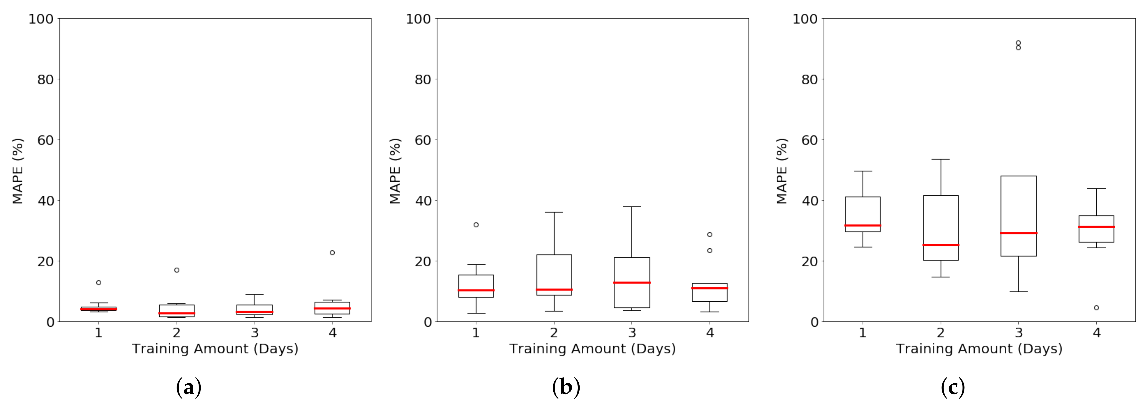
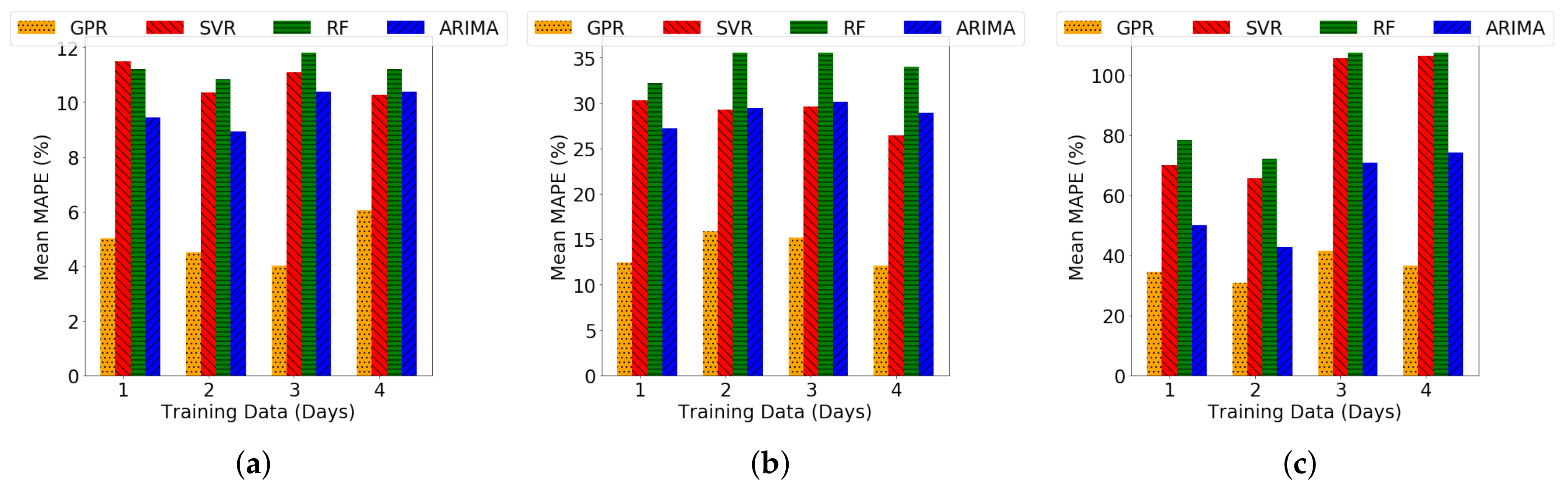
4.2.1. Long-Term Forecasting under Varying Duration of Training Data

We evaluate the prediction performance of our algorithm when there is varying duration of the training dataset. In this paper, we vary the training data from one day to four days and use these different trained models to predict the one day ahead energy load in the same week. We ran this evaluation on different weeks throughout the year and for each of the three datasets to predict the load for one day in each of these different weeks.
Figure 4 shows the spread of the Mean Absolute Percentage Errors (MAPE) for predicting next day load across different weeks for the different data that we have when tested using models trained on different amount of training data. It can be seen that there are certain boxplots missing a whisker. Whiskers on the top of the boxplot represent the largest data point that is less than the Q 3 + 1.5 ( Q 3 Q 1 ) , where Q3 is the 3rd quartile or the 75-percentile, Q1 is the 1st quartile of 25-percentile and Q 3 Q 1 represents the inter-quartile range, IQR [70]. Whiskers on the bottom of the boxplot represent the smallest point that is larger than Q 1 1.5 ( Q 3 Q 1 ) [70]. Any point above the top whisker and below the bottom whisker are conventionally considered to be “outlier points”. Thus, in Figure 4, the boxplots in the Y2E2 cooling load and Y2E2 lighting load that have no top whiskers indicate that there are no data points for MAPE values between Q3 and Q 3 + 1.5 ( Q 3 Q 1 ) , even with a larger dataset. Hence, if we can choose to look beyond these very few outliers, it can be seen that the median MAPE for CMU electricity load prediction is around 5% and for Y2E2 cooling load prediction, it is around 10% which are quite accurate. The error percentage is quite high for the Y2E2 lighting load, with the median error around 30%. This difference in error is due to the volatility of the lighting load. It is more difficult to predict the highly volatile load data because of the high uncertainty.
In this paper, we refer to volatility of the load as the degree of smoothness of the load curve. We quantify this degree of smoothness of the load curve by calculating the conventional metric of smoothness, namely the lag-one autocorrelation of the difference between the consecutive data points of the load. As this value approaches 1, it means that the curve is very smooth and it is said to be very jagged when it is near −1. Figure 1 and Figure 3 show that the Y2E2 lighting load is less smooth as compared to the CMU electricity load and Y2E2 cooling load. The lag-one autocorrelation values of the difference between the consecutive data points of the load curves in Figure 3 is 0.893, 0.799 and 0.336 for CMU electricity load, Y2E2 cooling load and Y2E2 lighting load, respectively. The smoothness in the CMU electric load can be attributed to the fact that it is the aggregated electricity consumption data of a group of ten buildings in the CMU campus (Section 4.1.1). Hence the turning on/off of a few appliances does not make a significant impact on the load curve. The Y2E2 cooling load is the amount of chilled water being used (in tons) to cool one building (Section 4.1.2). This HVAC load is always an incremental increase and it is not a sudden turn on/off and hence we fail to see any significant step ups/downs in the load profile. On the other hand, the Y2E2 electric load is just the power consumed by lighting appliances in the Y2E2 building (Section 4.1.2). Hence, it is not that large as the CMU aggregated electricity load and change in state of one or two lighting appliances can make a significant impact on the overall lighting load. Lighting loads can be turned off/on immediately and this feature can cause sudden step ups/downs in the load curve and hence it is less smooth compared to both of the other loads.
Then we compare the results we obtained using Gaussian Processes with other benchmark methods. Figure 5 plots the mean values of the MAPE obtained for the three loads after applying Gaussian Process Regression (GPR), Support Vector Regression (SVR), Random Forest (RF) and Autoregressive Integrated Moving Average (ARIMA). It can be seen that our method produces much better results than the other three methods in all the three loads for all training data amount. GPR performs up to 2.95 times, 2.81 times and 2.94 times better than the other methods for CMU electricity load, Y2E2 cooling load and Y2E2 lighting load respectively. The prior knowledge about the type of data is represented in the covariance kernel functions that we chose, and this decision helps the GPR to produce more accurate results with lesser amount of data. From these, it is evident that irrespective of the amount of training data, GPR performs better than the other methods. Specially, for CMU electric data, 3-days results in best performance for our GPR method. For Y2E2 cooling load and lighting load, 4-days and 2-days result in best performance for our GPR method respectively.

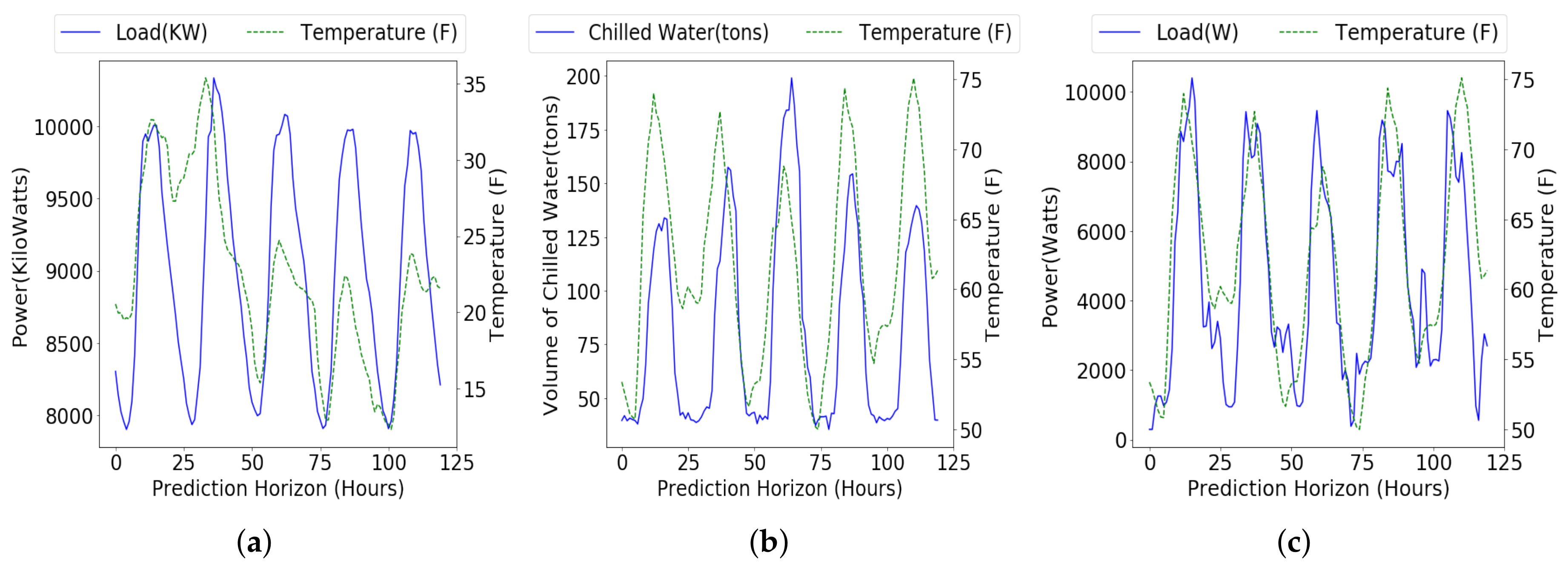
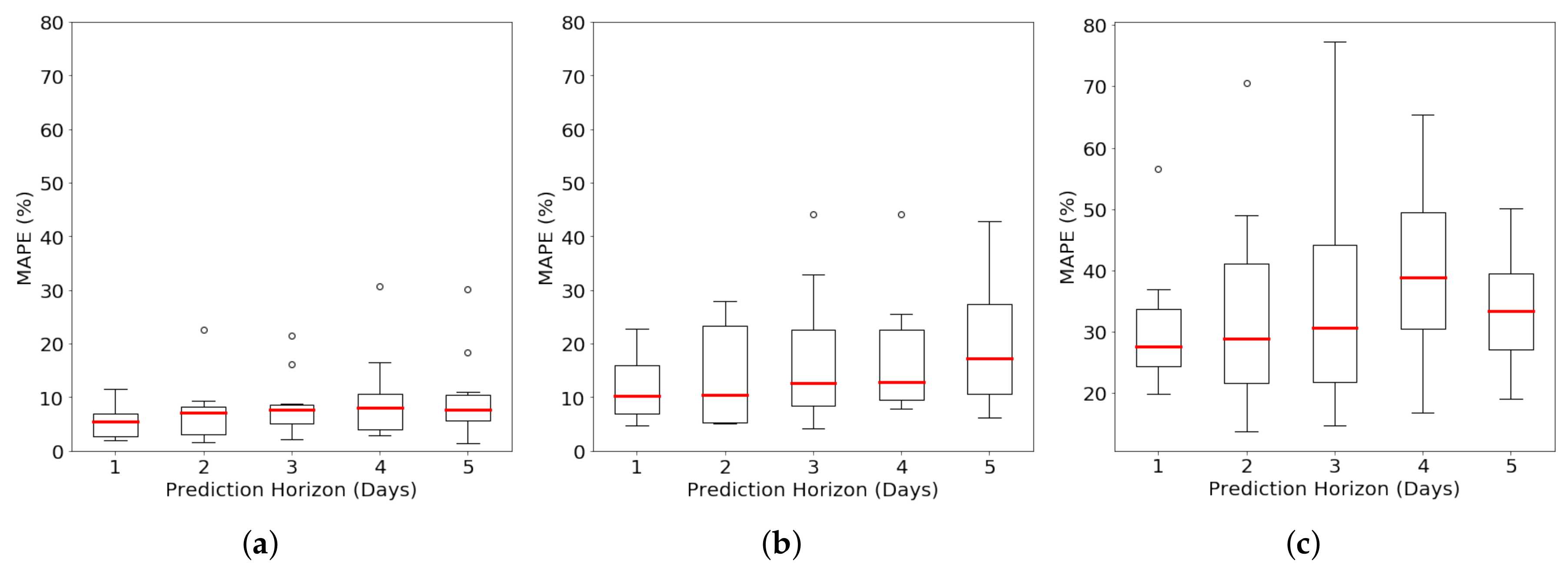
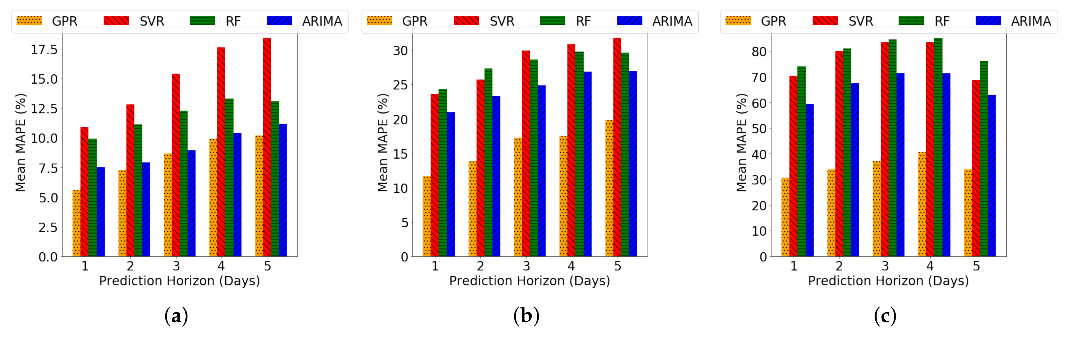
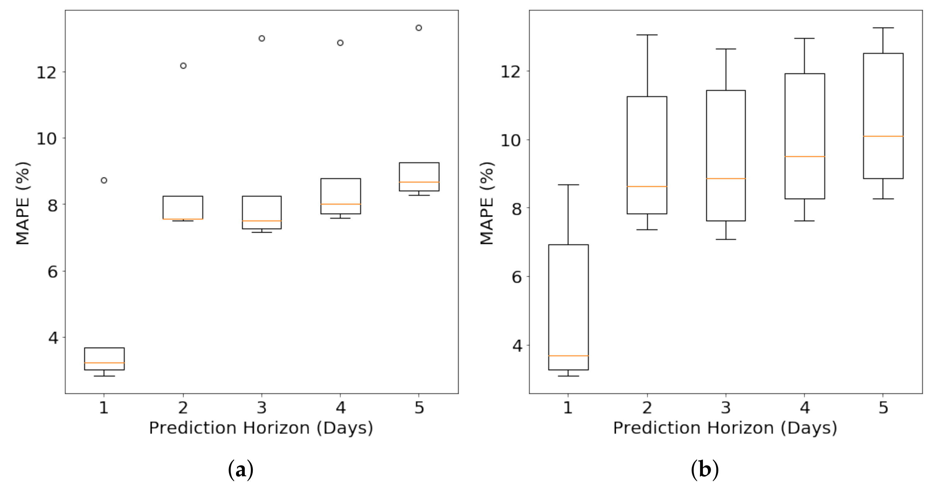
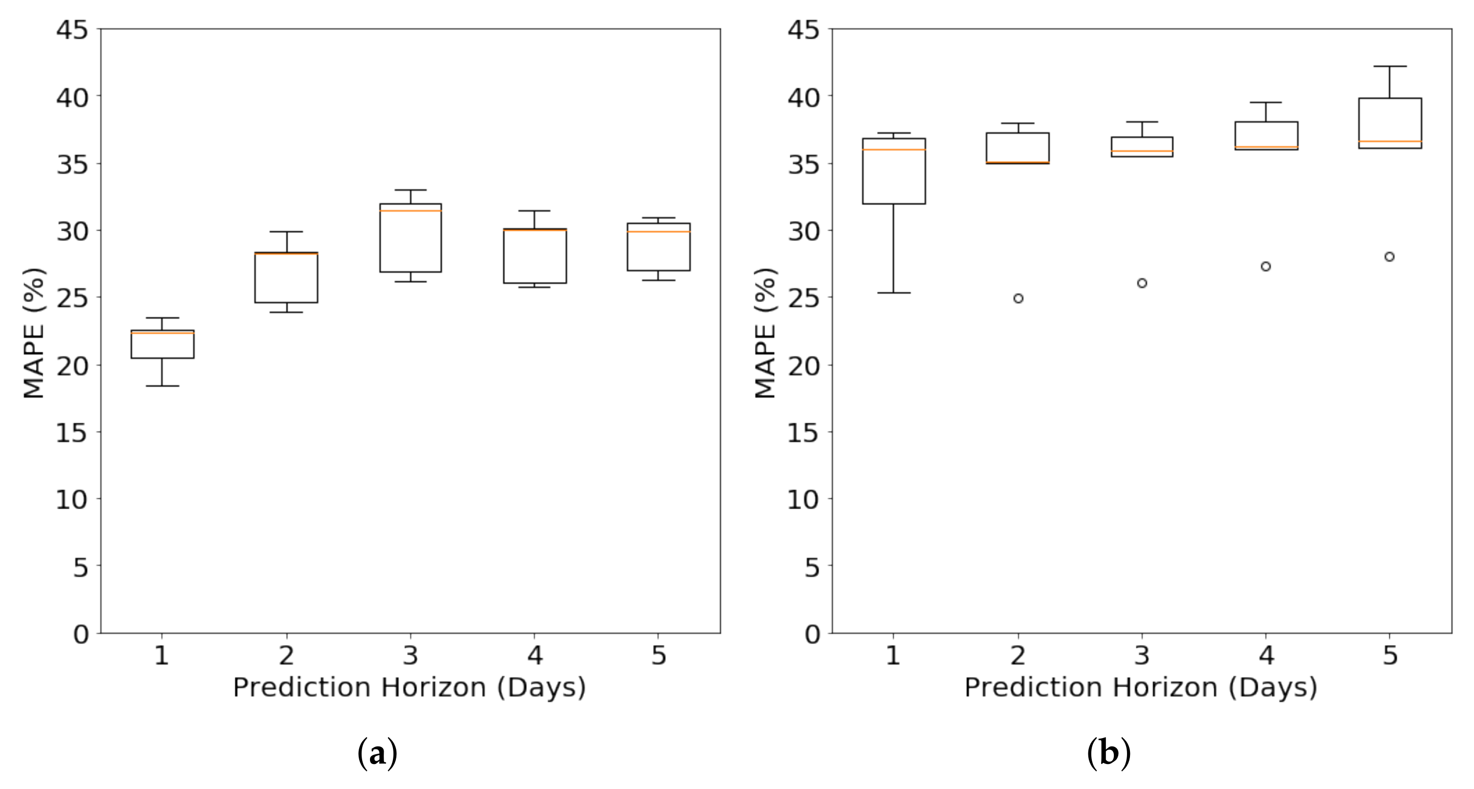
4.2.2. Long-Term Forecasting under Varying Prediction Horizon

In this section, we test the performance of our prediction models for all the different loads while varying the prediction horizon from one day to five days. By this evaluation, we can see how far ahead can our GPR model predict the future building energy consumption values accurately. For this evaluation, we use the models trained on 1 training day that had been presented in Section 4.2.1. The models are trained on one day of the week (could be any day) and are used to predict the load on its first day ahead, its second day ahead and up to its fifth day ahead. For example, when the prediction horizon is 1, a model trained on Monday of a week is used to predict the Tuesday’s load, a model trained on Tuesday is used to predict Wednesday’s load etc. When the prediction horizon is 3, in this example, the model trained on the Monday’s load would be used to predict Thursday’s load and the model trained on Tuesday would be used to predict Friday’s load and so on. This evaluation is also done across multiple weeks to get more data points and thus stable results.
Each boxplot in Figure 6 represents the distribution of the MAPE of prediction horizon of ‘k’ days (with ‘k’ varying from 1 to 5 days). CMU electricity load forecasting is very accurate with the median error percentage always less than 8%. The median Y2E2 cooling load error is less than 17% and the median MAPE for Y2E2 lighting load is less than 39%. The higher error for the Y2E2 lighting load can be attributed to the high volatility of the lighting load as mentioned in Section 4.2.1 and shown in Figure 1 and Figure 3. Both median and mean in Figure 6 and Figure 7 show a general trend of increasing MAPE values as the prediction horizon increases, with the exception of 5-day prediction horizon for Y2E2 lighting load. The decrease in the 5-day ahead lighting forecasting MAPE value may be due to the fact that (1) the 5-day ahead happened to have the same day of the week as the training and the test data (e.g., the GPR is trained on the load profile from Monday and tested on the next Monday data, because only weekdays are considered) and (2) the lighting load tends to be more sensitive to daily human activities compared to the other two loads.
Figure 7 compares the average of MAPE of prediction results by using GPR based on our proposed kernels, SVR, RF and ARIMA methods. It can be seen here also that our algorithm outperforms the other three methods for all the loads. GPR performs up to 1.93 times, 2.08 times and 2.42 times better than the other methods for CMU electricity load, Y2E2 cooling load and Y2E2 lighting load respectively. From these, it can be concluded that GPR can produce quite accurate prediction results for future load forecasts up to at least five days in advance, but at the same time, more often than not, the likelihood of obtaining similarly accurate results as we obtained with prediction horizon of 1 or 2 days reduces, due to a general trend of higher variances and outlier points.

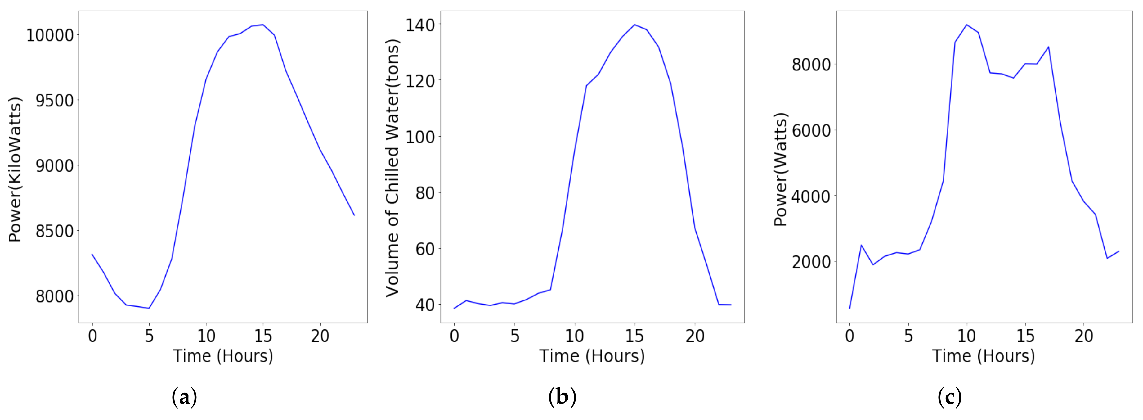
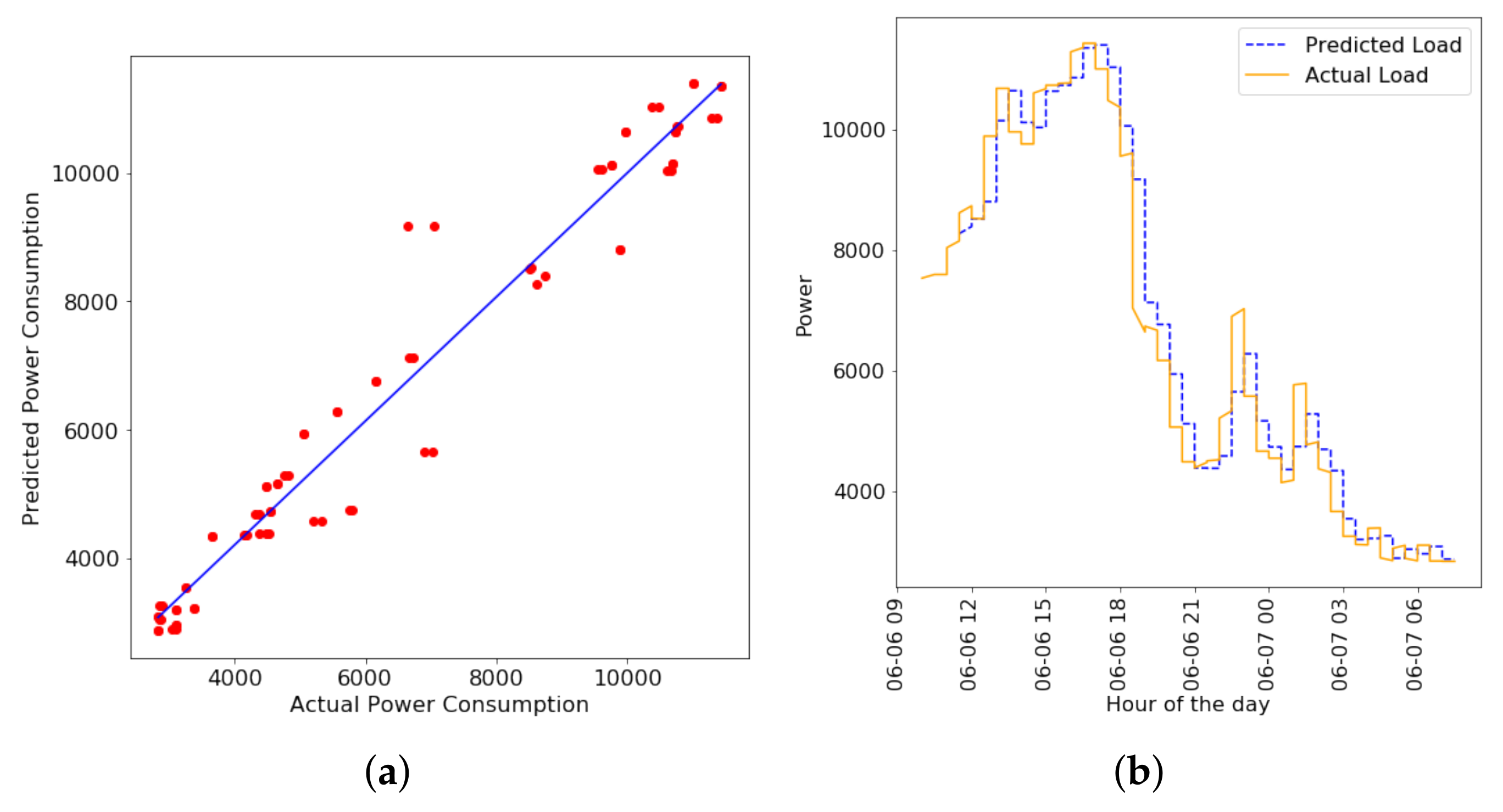
4.2.3. Short-Term Forecasting

We evaluate the performance of Gaussian Processes in short-term load forecasting. We used the kernel mentioned in Section 3.2.3, which is a linear kernel with noise. We used consumption and temperature data for the previous 30 min to predict the load data for the next 10 min. Figure 8a is a scatter plot of the actual against the predicted Y2E2 lighting load values for a 20 h period in a day. The actual and predicted time-series load is shown in Figure 8b and it can be seen from these two that, this short-term prediction algorithm using Gaussian Process Regression is quite accurate. The initial few data points in Figure 8b, where there is only actual load data and no predicted load data, are the first set of training data (30 min, which consists of 6 data points). These were used to train a model and predict the first two values on the predicted load curve. Now the next training period moves 10 min ahead from the initial start time and extends up to 30 more minutes. These points are then used to train a new model and predict the 2 values for next 10 min and this process continues. We obtained a low prediction MAPE of 7.96%, which is much better than the errors that we obtained on the Y2E2 lighting load with long term forecasting. Similarly, we obtained better prediction results with short-term forecasting of the CMU electricity load and Y2E2 cooling load as well, with MAPE of 0.735% and 6.53% respectively. Therefore it can be seen that with short-term, we are much more aware of the recent trends in data and it is easier to predict accordingly.

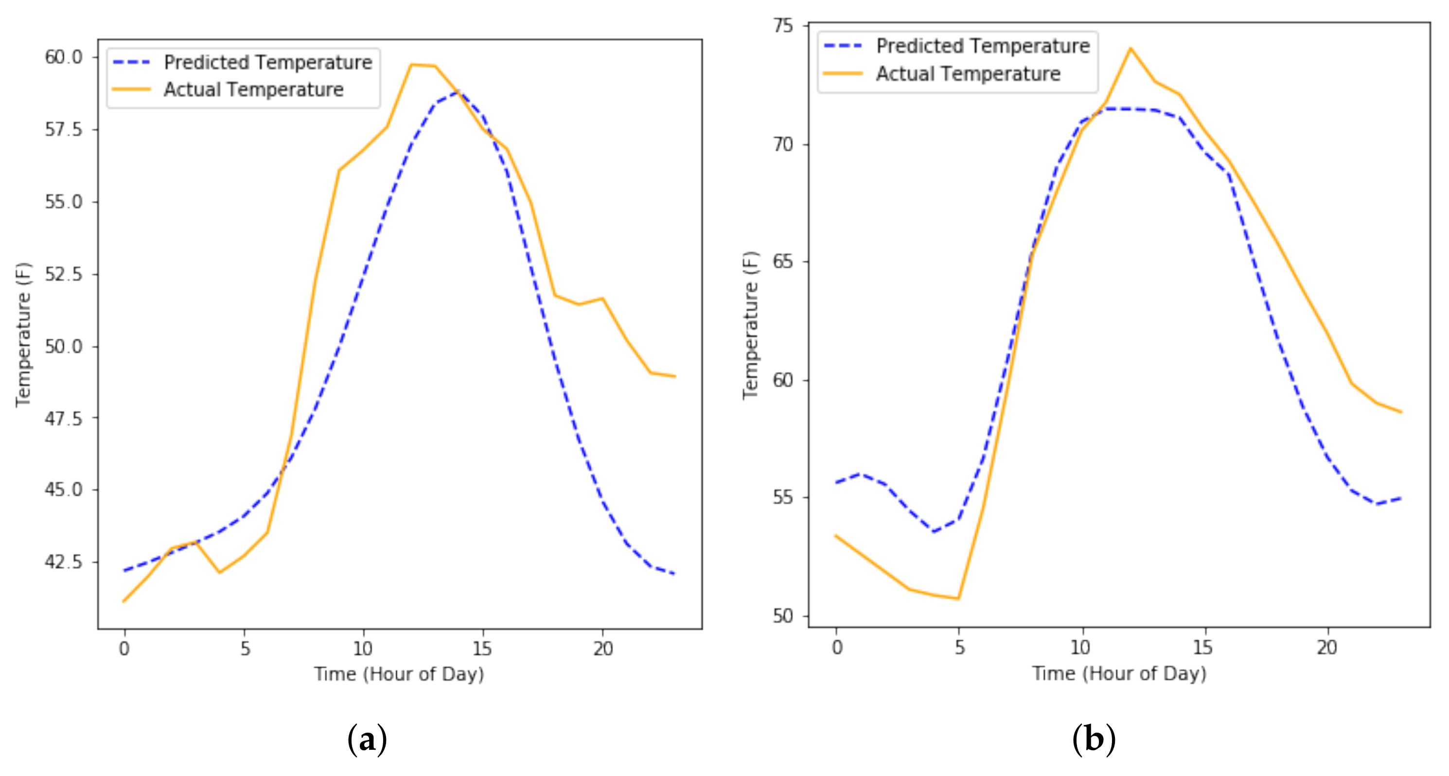
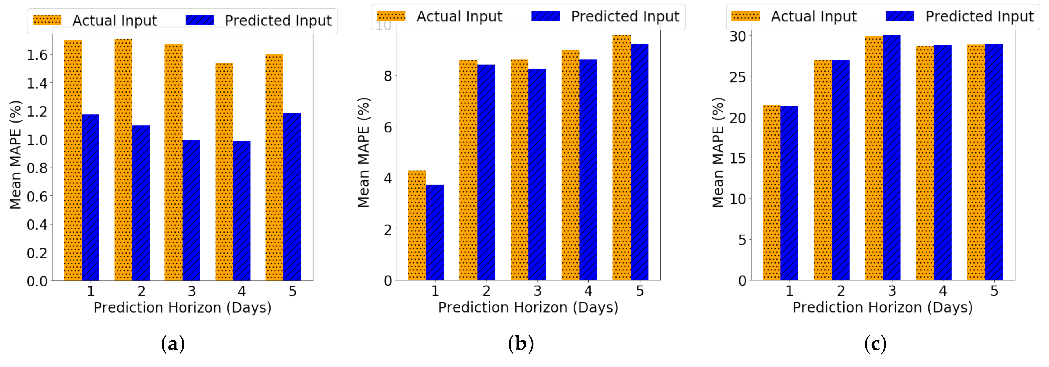
4.2.4. Long-Term Forecasting with Predicted Inputs

As we are using temperature as an external input to predict the building’s load, we would need an estimate of future temperature as well, particularly if we are forecasting the building’s load on a future date. While we have access to temperature and load for the training the prediction model, we require the temperature for the period for which we are predicting the load as well, which is not available at the time of prediction. For this purpose, we predict the temperature first using Gaussian Processes and we make use of a kernel that combines the linear kernel and the squared exponential kernel. This makes a good kernel for predicting temperature because the temperature profile throughout a day is relatively smooth, as supported by our observations. A couple of examples of these observations can be seen in the “Actual Temperature” curve in Figure 9. The linear kernel allows increases and decreases in the predicted temperature according to similar and corresponding variations in the corresponding historical actual temperature used in training. We trained the Gaussian Process Regression model with the combined kernel to obtain the estimation of the temperature for the entire prediction horizon. Then we feed the predicted temperature to the load forecasting model to obtain the future load consumption.
Figure 10a,b show that mean MAPE value with predicted inputs is lower than that with actual input for CMU electricity load and Y2E2 cooling load forecasts. The mean MAPE of the Y2E2 lighting load forecast does not change much with different temperature input (actual vs predicted). However, for electricity load and cooling load, we found that using prediction as input can produce lower error than using actual temperature as input. To better understanding the results, we characterize two examples of prediction results. As Figure 9 shows, the actual temperature is jagged and not very smooth, especially when compared to the predicted temperature. The difference in smoothness of the temperature curve is also supported when we take the lag-one autocorrelation of the difference of consecutive values in both temperature signals: for Figure 9a, the autocorrelation metric is 0.936 for the predicted temperature and 0.687 for the actual temperature and similarly, for Figure 9b, it is 0.871 and 0.799 for the predicted and actual temperature, respectively. Therefore, CMU electric load and Y2E2 cooling load profiles are smoother than the actual temperature data, while Y2E2 lighting load data is less smoother than the actual temperature data.
As Figure 10 shows, when the load data is smoother, the predicted input results in less error than the actual input (e.g., up to 41% change in mean MAPE in Figure 9a. This change is the ratio of the difference between the mean MAPEs for the actual and predicted inputs to the mean MAPE for the actual input), while when the load data is less smoother, the performance using the predicted temperature is similar with using the actual temperature (e.g., up to 4.4% and 0.63% changes in mean MAPE in Figure 9b,c, respectively). This indicates that smoother input may improve the prediction accuracy on smooth load data. This may be because the smoother temperature input already reduces the uncertainty induced by irrelevant but volatile influence factors, such as measurement noise. Note that the purpose of this study is to show that our method using the predicted temperature input performs comparatively to using the actual temperature input. This is important since when predicting loads in practice, it is difficult to obtain the actual future temperature data. Thus, our method allows us to predict energy loads accurately without having to know the actual future temperature data.

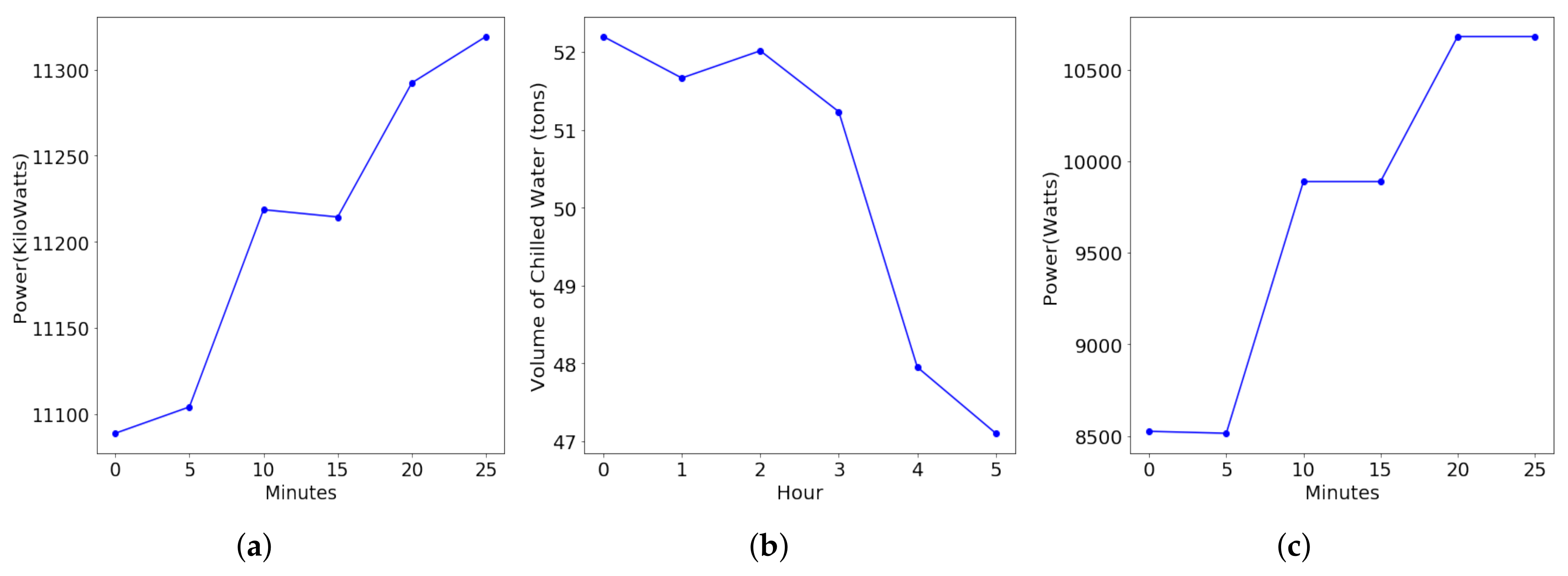
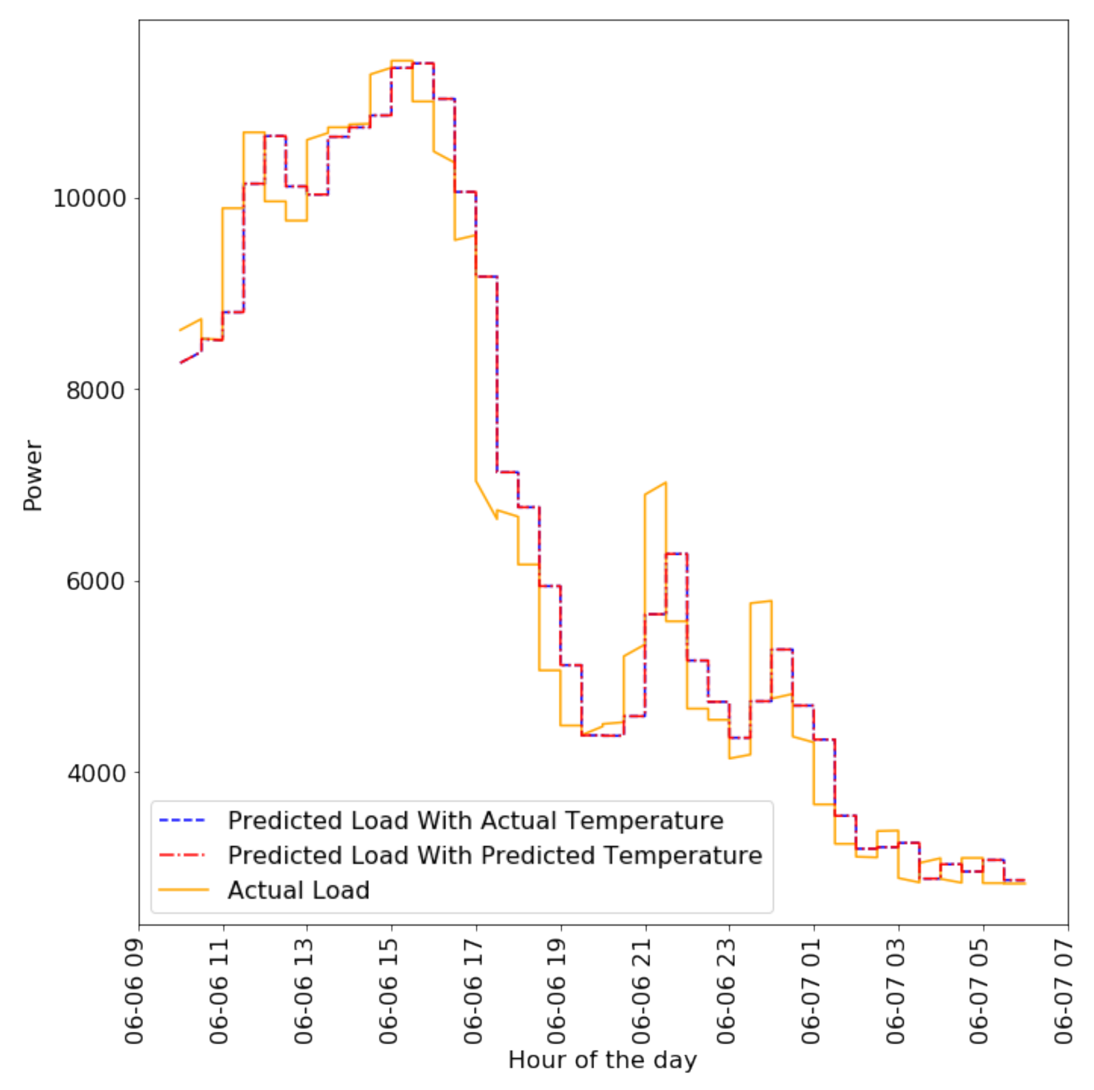
4.2.5. Short-Term Forecasting with Predicted Inputs

We evaluate the performance of our short term forecasting kernel, as mentioned in Section 3.2.3. Here we use the predicted temperature as inputs to the model instead of the actual temperature, as described in the above Section 4.2.4. We obtain the future temperature estimate using Gaussian Process and a combination of linear kernel and squared exponential kernel (as above) and use this estimate to predict the future load for a short term duration of 10 min. Similar to the short term forecasting earlier, we use 30 min of training data to obtain these 10 min of load forecasts.
Figure 11 shows the actual Y2E2 lighting load, predicted Y2E2 lighting load using actual temperature, and predicted Y2E2 lighting load using predicted temperature for a 20 h period in a day. It can be seen that both predicted load curves overlap each other. The MAPE of the load prediction with predicted temperature is 7.96%, which is almost exactly the same the MAPE of the load predicted with actual temperature (difference of 4 × 10 6 ). This is mainly due to the fact that in such a small duration of 10 min, the actual and predicted temperature differ only by around 0.3 F–0.5 F. The low error rate of temperature prediction make it feasible to use predicted temperature as the input for short term load forecasting.

4.2.6. Impacts of Different Kernels

We investigated the impacts of using different kernels, Matern kernel and combination of Matern kernel and linear kernel, on the performance of Gaussian Process Regression for load forecasting, compared to our method.
1.
Matern kernel for Y2E2 Building’s Cooling Load Forecasting
As the Matern kernel is another commonly used kernel for modeling the varying load consumption instead of the smoother squared exponential function, we predicted the cooling load for Y2E2 building for one to five days ahead using Matern Kernels (shown in Equation (13)) and compared the performance with that of the squared exponential kernel.
Matern Kernel resulted in a higher MAPE with a higher deviation as Figure 12 showed. This empirically justifies our kernel selection to use the squared exponential kernel for our GPR modeling. This is due to the smoothness associated with our load curve as we are taking the total consumption of a whole building, instead of a more granular level of consumption like a conference room or a small residential building. This smoothness can be better captured by the squared exponential curve and hence it produces a better load forecast.
2.
A combination of Matern and Linear Kernel for Y2E2 Building’s lighting load forecasting
We present the results of the Y2E2 lighting load forecast using the combination of Matern and linear kernels:
K ( x , x ) = θ 1 2 × ( x c ) × ( x c ) 2 1 ν Γ ( ν ) 2 ν ( x x ) l ν K ν 2 ν ( x x ) l + θ 2 2 δ x , x
where θ 1 , θ 2 , ν and l are hyper-parameters, K ν is a modified Bessel function, Γ ( ν ) is a Gamma function and δ i , j is the Kronecker Delta function for i and j [68]. We then compare the results with those of using our kernel model described in Section 3.2.2. We used lighting loads as it is the least smooth of the three data that we have.
Figure 13 shows that our kernel model performs much better (lower MAPE) than the combination of Matern and linear kernels developed to characterize not-so-smooth functions. While many more kernels can be constructed and compared, these results show that the more we understand the physical insights about the data and encode it in our covariance function, more accurate forecasting results will become.

5. Conclusions

This paper introduced a new building energy forecasting method that combines Gaussian Process Regression and physical insights and heuristics about load data in diverse forecasting scenarios. We investigated building energy load data for various durations and then modeled the covariance function of the GPR accordingly using kernels to represent the behavior of the data most accurately in each scenario. For example, long-term behavior of aggregate loads tend to be smooth and periodic over time, and thus smoother kernels, such as the squared exponential kernel and periodic functions, are more appropriate, while for short-term forecasting a simpler kernel-like linear kernel is more appropriate. The performance of our method is evaluated with three field datasets to predict loads in diverse forecasting scenarios, such as amount of training data, prediction horizon, load type, and aggregation level. The field datasets include aggregated electricity load of Carnegie Mellon University (CMU), the cooling and the lighting load of a campus building in Stanford University. The results show that as the amount of training data and the duration of prediction horizon increases, the overall prediction error increases. Our model resulted in the prediction accuracy of up to 94.38% and 99.26% for long- and short-term forecasting, respectively. They correspond to up to 2.95 times improvement in the prediction error, compared to state-of-the-art forecasting methods, including Support Vector Regression (SVR), Random Forest (RF), and Autoregressive Integrated Moving Average (ARIMA). The evaluations show that our Gaussian Process load forecasting model is accurate and robust to diverse forecasting scenarios using minimal training data.

Acknowledgments

We thank Facilities Management Services at Carnegie Mellon University for providing us access to the CMU aggregate electricity data.

Author Contributions

All authors have worked on developing the concept and validation. In particular, Hae Young Noh and Ram Rajagopal mostly focused on overall modeling. Anand Krishnan Prakash and Susu Xu focused on specific algorithm development and validation. All authors have worked on writing and revising the paper.

Conflicts of Interest

The authors declare no conflict of interest.

References

  1. Congressional Budget Office. How Much Does the Federal Government Support the Development and Production of Fuels and Energy Technologies? Available online: https://www.cbo.gov/publication/43040 (accessed on 31 January 2018).
  2. gov.uk. Environmental Taxes, Reliefs and Schemes for Businesses. Available online: https://www.gov.uk/green-taxes-and-reliefs (accessed on 31 January 2018).
  3. Kallakuri, C.; Vaidyanathan, S.; Kelly, M.; Cluett, R. The 2016 International Energy Efficiency Scorecard. 2016. Available online: http://habitatx.com/wp-content/uploads/2016/07/2016_ACEEE_country_report.pdf (accessed on 31 January 2018).
  4. United States Energy Information Administration. How Much Energy Is Consumed in U.S. Residential and Commercial Buildings? Available online: https://www.eia.gov/tools/faqs/faq.php?id=86&t=1 (accessed on 31 January 2018).
  5. United States Energy Information Administration. International Energy Outlook 2016. Available online: https://www.eia.gov/outlooks/ieo/pdf/0484(2016).pdf (accessed on 31 January 2018).
  6. Chen, D.; Irwin, D. SunDance: Black-box Behind-the-Meter Solar Disaggregation. In Proceedings of the Eighth International Conference on Future Energy Systems (e-Energy ’17), Shatin, Hong Kong, 16–19 May 2017; ACM: New York, NY, USA, 2017; pp. 45–55. [Google Scholar]
  7. Mohan, R.; Cheng, T.; Gupta, A.; Garud, V.; He, Y. Solar Energy Disaggregation using Whole-House Consumption Signals. In Proceedings of the 4th International Workshop on Non-Intrusive Load Monitoring (NILM), Austin, TX, USA, 7–8 March 2014. [Google Scholar]
  8. Li, X.; Wen, J. Review of building energy modeling for control and operation. Renew. Sustain. Energy Rev. 2014, 37, 517–537. [Google Scholar] [CrossRef]
  9. eQUEST: The QUick Energy Simulation Tool. 2016. Available online: http://www.doe2.com/equest/ (accessed on 31 January 2018).
  10. EnergyPlus. 2017. Available online: https://energyplus.net/ (accessed on 31 January 2018).
  11. Yang, Z.; Becerik-Gerber, B. A model calibration framework for simultaneous multi-level building energy simulation. Appl. Energy 2015, 149, 415–431. [Google Scholar] [CrossRef]
  12. Zhao, J.; Lasternas, B.; Lam, K.P.; Yun, R.; Loftness, V. Occupant behavior and schedule modeling for building energy simulation through office appliance power consumption data mining. Energy Build. 2014, 82, 341–355. [Google Scholar] [CrossRef]
  13. Fumo, N.; Mago, P.; Luck, R. Methodology to estimate building energy consumption using EnergyPlus Benchmark Models. Energy Build. 2010, 42, 2331–2337. [Google Scholar] [CrossRef]
  14. Azar, E.; Menassa, C. A conceptual framework to energy estimation in buildings using agent based modeling. In Proceedings of the 2010 Winter Simulation Conference, Baltimore, MD, USA, 5–8 December 2010; pp. 3145–3156. [Google Scholar]
  15. Yu, D. A two-step approach to forecasting city-wide building energy demand. Energy Build. 2018, 160, 1–9. [Google Scholar] [CrossRef]
  16. Amasyali, K.; El-Gohary, N.M. A review of data-driven building energy consumption prediction studies. Renew. Sustain. Energy Rev. 2018, 81, 1192–1205. [Google Scholar] [CrossRef]
  17. Zhao, H.-X.; Magoulès, F. A review on the prediction of building energy consumption. Renew. Sustain. Energy Rev. 2012, 16, 3586–3592. [Google Scholar] [CrossRef]
  18. Ahmad, A.; Hassan, M.; Abdullah, M.; Rahman, H.; Hussin, F.; Abdullah, H.; Saidur, R. A review on applications of ANN and SVM for building electrical energy consumption forecasting. Renew. Sustain. Energy Rev. 2014, 33, 102–109. [Google Scholar] [CrossRef]
  19. Yildiz, B.; Bilbao, J.; Sproul, A. A review and analysis of regression and machine learning models on commercial building electricity load forecasting. Renew. Sustain. Energy Rev. 2017, 73, 1104–1122. [Google Scholar] [CrossRef]
  20. Daut, M.A.M.; Hassan, M.Y.; Abdullah, H.; Rahman, H.A.; Abdullah, M.P.; Hussin, F. Building electrical energy consumption forecasting analysis using conventional and artificial intelligence methods: A review. Renew. Sustaina. Energy Rev. 2017, 70, 1108–1118. [Google Scholar] [CrossRef]
  21. Zhou, K.; Fu, C.; Yang, S. Big data driven smart energy management: From big data to big insights. Renew. Sustain. Energy Rev. 2016, 56, 215–225. [Google Scholar] [CrossRef]
  22. United States Energy Information Administration. Nearly Half of All U.S. Electricity Customers Have Smart Meters. Available online: https://www.eia.gov/todayinenergy/detail.php?id=34012 (accessed on 31 January 2018).
  23. United States Energy Information Administration. How Many Smart Meters Are Installed in the United States, and Who Has Them? Available online: https://www.eia.gov/tools/faqs/faq.php?id=108&t=3 (accessed on 31 January 2018).
  24. American Council for an Energy-Efficient Economy. Improving Access to Energy Usage Data. Available online: https://aceee.org/sector/local-policy/toolkit/utility-data-access (accessed on 31 January 2018).
  25. Noh, H.Y.; Rajagopal, R. Data-driven forecasting algorithms for building energy consumption. Proc. SPIE 2013, 8692, 86920T. [Google Scholar]
  26. Yang, Y.; Li, S.; Li, W.; Qu, M. Power load probability density forecasting using Gaussian process quantile regression. Appl. Energy 2017, 213, 499–509. [Google Scholar] [CrossRef]
  27. Lloyd, J.R. GEFCom2012 hierarchical load forecasting: Gradient boosting machines and Gaussian processes. Int. J. Forecast. 2014, 30, 369–374. [Google Scholar] [CrossRef]
  28. Atsawathawichok, P.; Teekaput, P.; Ploysuwan, T. Long term peak load forecasting in Thailand using multiple kernel Gaussian Process. In Proceedings of the 2014 11th International Conference on Electrical Engineering/Electronics, Computer, Telecommunications and Information Technology (ECTI-CON), Nakhon Ratchasima, Thailand, 14–17 May 2014; pp. 1–4. [Google Scholar]
  29. Lauret, P.; David, M.; Calogine, D. Nonlinear Models for Short-time Load Forecasting. Energy Procedia 2012, 14, 1404–1409. [Google Scholar] [CrossRef]
  30. Neto, A.H.; Fiorelli, F.A.S. Comparison between detailed model simulation and artificial neural network for forecasting building energy consumption. Energy Build. 2008, 40, 2169–2176. [Google Scholar] [CrossRef]
  31. Yezioro, A.; Dong, B.; Leite, F. An applied artificial intelligence approach towards assessing building performance simulation tools. Energy Build. 2008, 40, 612–620. [Google Scholar] [CrossRef]
  32. Balcomb, J.D.; Crowder, R.S. ENERGY-10, A Design Tool Computer Program for Buildings. In Proceedings of the American Solar Energy Society’s 20th Passive Solar Conference (Solar ’95), Minneapolis, MN, USA, 15–20 July 1995. [Google Scholar]
  33. Wang, S.; Xu, X. Parameter estimation of internal thermal mass of building dynamic models using genetic algorithm. Energy Convers. Manag. 2006, 47, 1927–1941. [Google Scholar] [CrossRef]
  34. Mena, R.; Rodríguez, F.; Castilla, M.; Arahal, M. A prediction model based on neural networks for the energy consumption of a bioclimatic building. Energy Build. 2014, 82, 142–155. [Google Scholar] [CrossRef]
  35. Agarwal, A.; Munigala, V.; Ramamritham, K. Observability: A Principled Approach to Provisioning Sensors in Buildings. In Proceedings of the 3rd ACM International Conference on Systems for Energy-Efficient Built Environments (BuildSys ’16), Stanford, CA, USA, 15–17 November 2016; ACM: New York, NY, USA, 2016; pp. 197–206. [Google Scholar]
  36. Jetcheva, J.G.; Majidpour, M.; Chen, W.P. Neural network model ensembles for building-level electricity load forecasts. Energy Build. 2014, 84, 214–223. [Google Scholar] [CrossRef]
  37. Kwok, S.S.; Lee, E.W. A study of the importance of occupancy to building cooling load in prediction by intelligent approach. Energy Convers. Manag. 2011, 52, 2555–2564. [Google Scholar] [CrossRef]
  38. Xuemei, L.; Yuyan, D.; Lixing, D.; Liangzhong, J. Building cooling load forecasting using fuzzy support vector machine and fuzzy C-mean clustering. In Proceedings of the 2010 International Conference on Computer and Communication Technologies in Agriculture Engineering, Chengdu, China, 12–13 June 2010; Volume 1, pp. 438–441. [Google Scholar]
  39. Dagnely, P.; Ruette, T.; Tourwé, T.; Tsiporkova, E.; Verhelst, C. Predicting Hourly Energy Consumption. Can Regression Modeling Improve on an Autoregressive Baseline? In Proceedings of the Third ECML PKDD Workshop on Data Analytics for Renewable Energy Integration, Porto, Portugal, 11 September 2015; Springer-Verlag: New York, NY, USA, 2015; Volume 9518, pp. 105–122. [Google Scholar]
  40. Huang, S.; Zuo, W.; Sohn, M.D. A Bayesian Network model for predicting cooling load of commercial buildings. Build. Simul. 2017, 11, 87–101. [Google Scholar] [CrossRef]
  41. Dudek, G. Short-Term Load Forecasting Using Random Forests. In Proceedings of the Intelligent Systems’2014, Warsaw, Poland, 24–26 September 2014; Springer International Publishing: Cham, Switzerland, 2015; pp. 821–828. [Google Scholar]
  42. Lahouar, A.; Slama, J.B.H. Random forests model for one day ahead load forecasting. In Proceedings of the IREC2015 The Sixth International Renewable Energy Congress, Sousse, Tunisia, 24–26 March 2015; pp. 1–6. [Google Scholar]
  43. Massana, J.; Pous, C.; Burgas, L.; Melendez, J.; Colomer, J. Short-term load forecasting for non-residential buildings contrasting artificial occupancy attributes. Energy Build. 2016, 130, 519–531. [Google Scholar] [CrossRef]
  44. Fernández, I.; Borges, C.E.; Penya, Y.K. Efficient building load forecasting. In Proceedings of the 2011 IEEE 16th Conference on Emerging Technologies & Factory Automation (ETFA 2011), Toulouse, France, 5–9 September 2011; pp. 1–8. [Google Scholar]
  45. Xuemei, L.; Lixing, D.; Jinhu, L.; Gang, X.; Jibin, L. A Novel Hybrid Approach of KPCA and SVM for Building Cooling Load Prediction. In Proceedings of the 2010 Third International Conference on Knowledge Discovery and Data Mining, Phuket, Thailand, 9–10 January 2010. [Google Scholar]
  46. Fan, C.; Xiao, F.; Wang, S. Development of prediction models for next-day building energy consumption and peak power demand using data mining techniques. Appl. Energy 2014, 127, 1–10. [Google Scholar] [CrossRef]
  47. Hagan, M.T.; Behr, S.M. The Time Series Approach to Short Term Load Forecasting. IEEE Trans. Power Syst. 1987, 2, 785–791. [Google Scholar] [CrossRef]
  48. Pai, P.F.; Hong, W.C. Support vector machines with simulated annealing algorithms in electricity load forecasting. Energy Convers. Manag. 2005, 46, 2669–2688. [Google Scholar] [CrossRef]
  49. Soares, L.J.; Medeiros, M.C. Modeling and forecasting short-term electricity load: A comparison of methods with an application to Brazilian data. Int. J. Forecast. 2008, 24, 630–644. [Google Scholar] [CrossRef]
  50. O’Neill, Z. Development of a Probabilistic Graphical Energy Performance Model for an Office Building. ASHRAE Trans. 2014, 120. [Google Scholar]
  51. O’Neill, Z.; O’Neill, C. Development of a probabilistic graphical model for predicting building energy performance. Appl. Energy 2016, 164, 650–658. [Google Scholar] [CrossRef]
  52. Jensen, K.L.; Toftum, J.; Friis-Hansen, P. A Bayesian Network approach to the evaluation of building design and its consequences for employee performance and operational costs. Build. Environ. 2009, 44, 456–462. [Google Scholar] [CrossRef]
  53. Sheng, H.; Xiao, J.; Cheng, Y.; Ni, Q.; Wang, S. Short-Term Solar Power Forecasting Based on Weighted Gaussian Process Regression. IEEE Trans. Ind. Electron. 2018, 65, 300–308. [Google Scholar] [CrossRef]
  54. Cheng, F.; Yu, J.; Xiong, H. Facial Expression Recognition in JAFFE Dataset Based on Gaussian Process Classification. IEEE Trans. Neural Netw. 2010, 21, 1685–1690. [Google Scholar] [CrossRef] [PubMed]
  55. Zhang, Y.; Yeung, D.Y. Multi-task warped Gaussian process for personalized age estimation. In Proceedings of the 2010 IEEE Computer Society Conference on Computer Vision and Pattern Recognition, San Francisco, CA, USA, 13–18 June 2010; pp. 2622–2629. [Google Scholar]
  56. Deisenroth, M.P.; Fox, D.; Rasmussen, C.E. Gaussian Processes for Data-Efficient Learning in Robotics and Control. IEEE Trans. Pattern Anal. Mach. Intell. 2015, 37, 408–423. [Google Scholar] [CrossRef] [PubMed] [Green Version]
  57. Ko, J.; Klein, D.J.; Fox, D.; Haehnel, D. Gaussian Processes and Reinforcement Learning for Identification and Control of an Autonomous Blimp. In Proceedings of the 2007 IEEE International Conference on Robotics and Automation, Roma, Italy, 10–14 Apirl 2007; pp. 742–747. [Google Scholar]
  58. Nguyen-Tuong, D.; Peters, J. Local Gaussian process regression for real-time model-based robot control. In Proceedings of the 2008 IEEE/RSJ International Conference on Intelligent Robots and Systems, Nice, France, 22–26 September 2008; pp. 380–385. [Google Scholar]
  59. Urtasun, R.; Fleet, D.J.; Fua, P. 3D People Tracking with Gaussian Process Dynamical Models. In Proceedings of the 2006 IEEE Computer Society Conference on Computer Vision and Pattern Recognition (CVPR’06), New York, NY, USA, 17–22 June 2006; Volume 1, pp. 238–245. [Google Scholar]
  60. Marquand, A.; Howard, M.; Brammer, M.; Chu, C.; Coen, S.; Mourão-Miranda, J. Quantitative prediction of subjective pain intensity from whole-brain fMRI data using Gaussian processes. NeuroImage 2010, 49, 2178–2189. [Google Scholar] [CrossRef] [PubMed]
  61. Challis, E.; Hurley, P.; Serra, L.; Bozzali, M.; Oliver, S.; Cercignani, M. Gaussian process classification of Alzheimer’s disease and mild cognitive impairment from resting-state fMRI. NeuroImage 2015, 112, 232–243. [Google Scholar] [CrossRef] [PubMed]
  62. Ziegler, G.; Ridgway, G.; Dahnke, R.; Gaser, C. Individualized Gaussian process-based prediction and detection of local and global gray matter abnormalities in elderly subjects. NeuroImage 2014, 97, 333–348. [Google Scholar] [CrossRef] [PubMed]
  63. Rasmussen, C.E.; Williams, C.K.I. Gaussian Processes for Machine Learning; MIT Press: Cambridge, MA, USA, 2006; Volume 1. [Google Scholar]
  64. Bhinge, R.; Park, J.; Law, K.H.; Dornfeld, D.A.; Helu, M.; Rachuri, S. Toward a Generalized Energy Prediction Model for Machine Tools. J. Manuf. Sci. Eng. 2016, 139, 041013. [Google Scholar] [CrossRef] [PubMed]
  65. Neal, R.M. Bayesian Learning for Neural Networks; Springer-Verlag: Secaucus, NJ, USA, 1996. [Google Scholar]
  66. Duvenaud, D. The Kernel Cookbook: Advice on Covariance Functions. Available online: http://www.cs.toronto.edu/~duvenaud/cookbook/index.html (accessed on 31 January 2018).
  67. Abramowitz, M.; Stegun, I.A. Handbook of Mathematical Functions; Dover Publications, Inc.: New York, NY, USA, 1972. [Google Scholar]
  68. Eric, W.; Weisstein. Kronecker Delta. From MathWorld—A Wolfram Web Resource. 2016. Available online: http://mathworld.wolfram.com/KroneckerDelta.html (accessed on 31 January 2018).
  69. Klessig, R.; Polak, E. Efficient implementations of the Polak-Ribiere conjugate gradient algorithm. SIAM J. Control 1972, 10, 524–549. [Google Scholar] [CrossRef]
  70. matplotlib, 2018. Available online: https://matplotlib.org/api/_as_gen/matplotlib.pyplot.boxplot.html (accessed on 31 March 2018).
Figure 1. Different 5-day loads and temperatures. (a) Aggregate Electricity Load and Temperature of Carnegie Mellon University; (b) Cooling load and Temperature for Y2E2 building in Stanford Campus; (c) Lighting load and Temperature for Y2E2 building in Stanford Campus.
Energies 11 00862 g001
Figure 2. Different loads for a short duration of time. (a) Aggregate Electricity Load of Carnegie Mellon University; (b) Cooling load for Y2E2 building in Stanford Campus; (c) Lighting load for Y2E2 building in Stanford Campus.
Energies 11 00862 g002
Figure 3. A Daily Load Profile for each of the dataset. (a) CMU electricity load; (b) Y2E2 cooling load; (c) Y2E2 lighting load.
Energies 11 00862 g003
Figure 4. Distribution of the prediction MAPE over different weeks for varying duration of training data using GPR. (a) CMU electricity load; (b) Y2E2 cooling load; (c) Y2E2 lighting load.
Energies 11 00862 g004
Figure 5. Mean of the MAPE of prediction over different weeks for varying duration of training data using GPR, SVR, RF and ARIMA. (a) CMU electric load; (b) Y2E2 cooling load; (c) Y2E2 lighting load.
Energies 11 00862 g005
Figure 6. Distribution of the prediction MAPE over different duration of training data for varying duration of prediction horizons using GPR. (a) CMU electricity load; (b) Y2E2 cooling load; (c) Y2E2 lighting load.
Energies 11 00862 g006
Figure 7. Mean of the MAPE of prediction over duration of training data for varying duration of prediction horizon using GPR, SVR, RF and ARIMA. (a) CMU electricity load; (b) Y2E2 cooling load; (c) Y2E2 lighting load.
Energies 11 00862 g007
Figure 8. Short Term Forecasting of the Y2E2 lighting load every 30 min period using a linear kernel in GPR. (a) Actual v/s Predicted Load for a 20 h period; (b) Predicted (blue dashed) and Actual (orange solid) load for a 20 h period.
Energies 11 00862 g008
Figure 9. A smooth predicted (blue dashed curve) and a jagged actual (orange solid curve) Temperature curve for two different days in Stanford, CA. (a) Day 1; (b) Day 2.
Energies 11 00862 g009
Figure 10. Mean of the MAPE of prediction when using Actual Temperature Input v/s Predicted Temperature Input in the GPR model for all the three loads. (a) CMU electricity load; (b) Y2E2 cooling load; (c) Y2E2 lighting load.
Energies 11 00862 g010
Figure 11. Actual Y2E2 lighting load (orange solid line), Short Term Forecast of the Y2E2 lighting load using Actual Temperature Input (blue dashed line) and Short Term Forecast of the same load using predicted Temperature Input (red dashed-dotted line) for a 20 h period.
Energies 11 00862 g011
Figure 12. MAPE for forecasting a Y2E2 cooling load chilled water consumption using Squared Exponential Kernel and Matern Kernel. (a) Squared Exponential Kernel; (b) Matern Kernel.
Energies 11 00862 g012
Figure 13. MAPE for forecasting the Y2E2 lighting load using our long-term load forecasting kernel (Section 3.2.2) and a combination of a linear and matern kernel. (a) Our long Term Load Forecasting Kernel in Section 3.2.2; (b) Combination of Matern and linear kernels for Long Term Forecasting.
Energies 11 00862 g013

