Optimal Load-Tracking Operation of Grid-Connected Solid Oxide Fuel Cells through Set Point Scheduling and Combined L1-MPC Control

Abstract

An optimal load-tracking operation strategy for a grid-connected tubular solid oxide fuel cell (SOFC) is studied based on the steady-state analysis of the system thermodynamics and electrochemistry. Control of the SOFC is achieved by a two-level hierarchical control system. In the upper level, optimal setpoints of output voltage and the current corresponding to unit load demand is obtained through a nonlinear optimization by minimizing the SOFC’s internal power waste. In the lower level, a combined L1-MPC control strategy is designed to achieve fast set point tracking under system nonlinearities, while maintaining a constant fuel utilization factor. To prevent fuel starvation during the transient state resulting from the output power surging, a fuel flow constraint is imposed on the MPC with direct electron balance calculation. The proposed control schemes are testified on the grid-connected SOFC model.

1. Introduction

The globally exploding capacity of renewable energy during the past decade makes a remarkable contribution to the conservation of fossil-fuel energy resources and an increasing number of distributed generations (DGs). However, the intermittent energy sources, such as solar energy and wind energy connected to the power grid, brings severe shortage of peaking regulation capacity, which has become the major factor that limits the further promotion of these renewable energies. To this end, seeking for new peaking regulation units have become a renewed issue in the field of power and energy engineering in recent years. It is reported that some large scale thermal power plants are incorporated into the peaking units recently through a series of technical reformation [1,2]. However, the variable load operation would have a negative impact on the efficiency of thermal power plants and brings extra cost to the maintenance [3]. In the recent years, the academia realize that electrolytic hydrogen making combined with hydrogen storage might be a promising solution to address the challenge brought from renewable energies [4,5]. As a complementary technology for hydrogen energy storage, solid oxide fuel cells (SOFCs) has drawn a lot of attention these years for its high efficiency of energy conversion and is treated as a candidate for peaking power plant when being connected to a power gird due to its capability for fast power response.

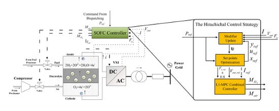
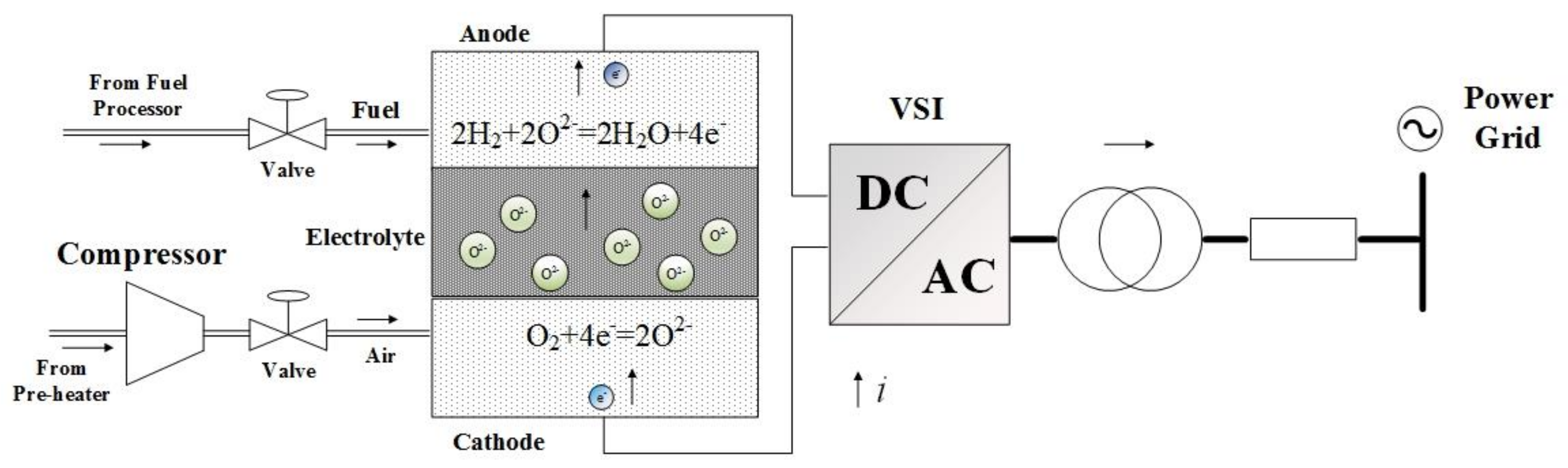
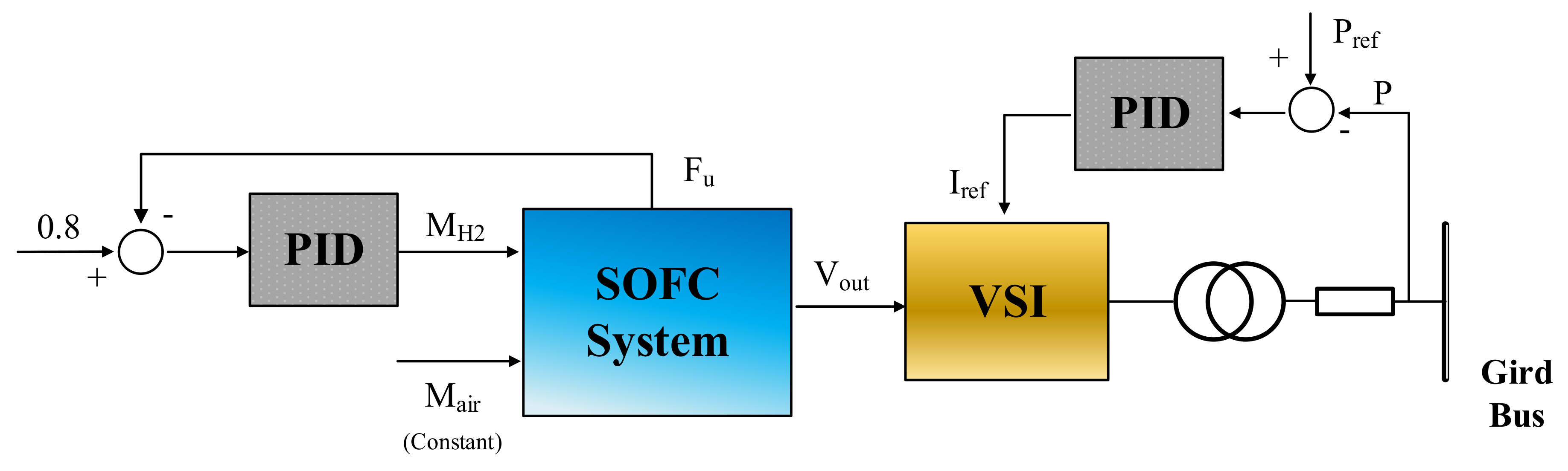
Omitting the preheaters and the fuel processers, Figure 1 gives a brief schematic diagram of a grid-connected SOFC that is discussed in this paper. The fuel (hydrogen) and the oxidant (usually oxygen from compressed air) are fed into the anode and cathode, respectively. The electrochemical reaction takes place at the electrolyte and produces electric potentials. The reaction is

Anode:	$2H_2+2O^{2-}\to 2H_{2}O+4e^{-}$
Cathode:	$O_2+4e^{-}\to 2O^{2-}$
Overall reaction:	$2H_2+O_2\to 2H_{2}O$

When the circuit loop is closed, the reaction proceeds to output electric power to the external load. In practice, SOFCs are usually connected to a micro power grid through voltage source invertors (VSI) for DC-AC transformation. In the grid level, the dispatching system is working to generate load demand signals to the power sources that are connected to the grid. These power sources make response to the load demands, thus the energy are balanced in the power grid and the frequency are maintained [6]. Consequently, for grid-connected SOFCs, its output power should track the unit load demand from the dispatching system. With this operation mode, the control problem considered for a grid-connected SOFC lies in:

• As peaking power plant, the SOFC system should have fast load variation ability to compensate the power fluctuation from intermittent energies in the gird. In other words, the peaking SOFC systems are expected to have a fast response to the unit load demand.
• When the SOFC operates in a steady state, the system efficiency should be optimized in order to exploit for the maximum profit. An explicit for the efficiency is the ratio of the output electrical power to the chemical power that is released by the fuel, which implies that with a specific output power, the maximum of the efficiency is equivalent to the minimum of the heating power that is wasted with the cells’ internal resistance.
• The dynamic of SOFC system takes on a strong nonlinearity under various operating conditions. Since the performance of linear controllers would deteriorate seriously when the system deviates from the nominal design condition, the control system should have the ability to handle the nonlinearity.
• The system constraints, referring to the limitations of system variables associated with the physical property and safety requirements should be fulfilled during both the transient process and steady-state operation. Among the constraints of SOFC system, fuel utilization (FU) is the most critical one for the system safety. In the first place, an overused fuel condition (FU > 0.9), namely fuel starvation, should be strictly avoided. The reason is that the fuel provides a reducing atmosphere for the electrodes under the operational condition of high temperature inside the SOFC. Lack of fuel gas would break the reducing atmosphere. In this case, the anode materials would be oxidized, triggering a permanent damage of the SOFC [7]. Low FU is accepted in the transient process, but a long-term low FU operation dramatically increases the fuel cost, thus causing a low efficiency of SOFC system. Most of the existing research literatures suggest that the FU should be controlled at 0.8 during the steady-state operation and within the range of 0.7 to 0.9 during the transient state for a comprehensive consideration both on safety and economy [8].

The intention of the paper is to put forward an integrated control system design attempting to meet the above requirements for a grid-connected SOFC system. In industrial processes, a classical solution to optimal operation is to adopt a hierarchical strategy in the control system design. The control system is divided into two levels, an upper level, with set point scheduler, and a lower level, with tracking controller. The set point scheduler performs an optimization on the basis of a rigorous steady-state model of the plant and feeds the lower level controller with setpoints corresponding to the optimization results [9,10]. It is of course that a complicated model with as more detail as possible is preferred for better optimization results. On the other hand, an excessively complicated model is disadvantageous for controller design, resulting in increasing cost for the implementation of controller and decreasing system reliability. The advantage of hierarchical control structure is that it separates the optimization problem and control problem. The separation of the two problems regarded in optimal operation enables the optimizer and the controller to be designed individually without being concerned by incorporation of each other. Benefiting from the merits discussed above, this hierarchical control is naturally treated as a candidate employed for achieving optimal operation of SOFC. However, as far as the authors’ knowledge, such study conducted in a SOFC operation study is still limited.

Making a general survey of mainstream control algorithm for tracking controller in the lower level, Model Predictive Control (MPC) appears to be the most powerful and convenient one to deal with system constraints [11,12,13,14]. Some studies on the application of MPC to a SOFC control problem have been performed previously [8,15,16,17]. These designs used varieties of nonlinear models in the MPC formulation to accommodate the nonlinearities. However, extensive online computation for nonlinear MPC limits its suitability for a time-sensitive system as grid-connected SOFCs. Previous works proposed an Active Disturbance Rejection Control (ADRC), which cooperated with MPC to handle the nonlinearity with acceptable computation [18]. Despite a given voltage being followed, the FU was not able to be maintained at the expected constant. It is believed that a direct modification of this control algorithm for maintaining a constant FU is difficult, due to the inability of the ADRC algorithm for multi-input-multi-output (MIMO) systems. To meet the requirement for voltage control and constant FU maintaining simultaneously, L1 Adaptive Control (L1AC) will be employed to work in combination with MPC, which will be referred as L1-MPC in this paper. The L1 Adaptive Control is a robust adaptive control algorithm developed from the model reference adaptive control (MRAC) algorithm. In the philosophy of the L1AC algorithm, it treats the nonlinearity, disturbance, and unknown parameters of the system as a lumped uncertainty term in the model. The lumped uncertainty term is estimated with a fast adaptive law and a compensation term is included in L1AC’s control law. With the fast adaptation mechanism, the closed-loop system with L1AC approaches a given reference model. In [19,20,21], theoretical analysis has been given to show the guarantee of the transient error between the closed-loop system and reference model. Although the proposer of L1AC mainly shed light on the state feedback algorithms and the existing output feedback L1AC algorithm is only for single-input-single-output (SISO) system [19], it is convenient to extend the SISO L1AC algorithm to a MIMO one.

In this paper, we present a hierarchical control strategy for grid-connected SOFC. In the upper level, set points of output voltage and current corresponding to unit load demand are obtained through solving a nonlinear optimization problem for the maximum efficiency of SOFC in steady-state operation. Steady-state analysis of a tubular SOFC is carried out in advance to formulate the optimization problem. In the lower level, a L1-MPC tracking controller with a combination of MIMO output feedback L1AC and MPC is put forward to steer the output variables to their optimal set points, handling all of the nonlinearities and constraints. To ensure the avoidance of fuel starvation, additional protection logic is designed afterwards.

The rest of this paper is organized as follows. In Section 2, several dynamic SOFC models are first reviewed to choose the most proper dynamic model for the control study in this work. Then, steady-steady analysis of a tubular SOFC is presented. Section 3 establishes the hierarchical control architecture with set point scheduler and the L1-MPC based tracking controller. Simulation results are given in Section 4. Finally, conclusions and future works are presented in Section 5.

2. Review of SOFC Structures and Models

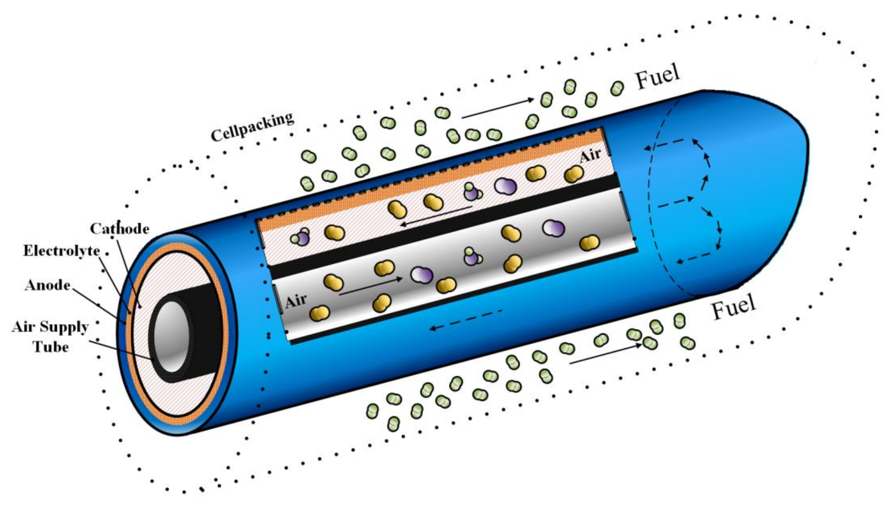
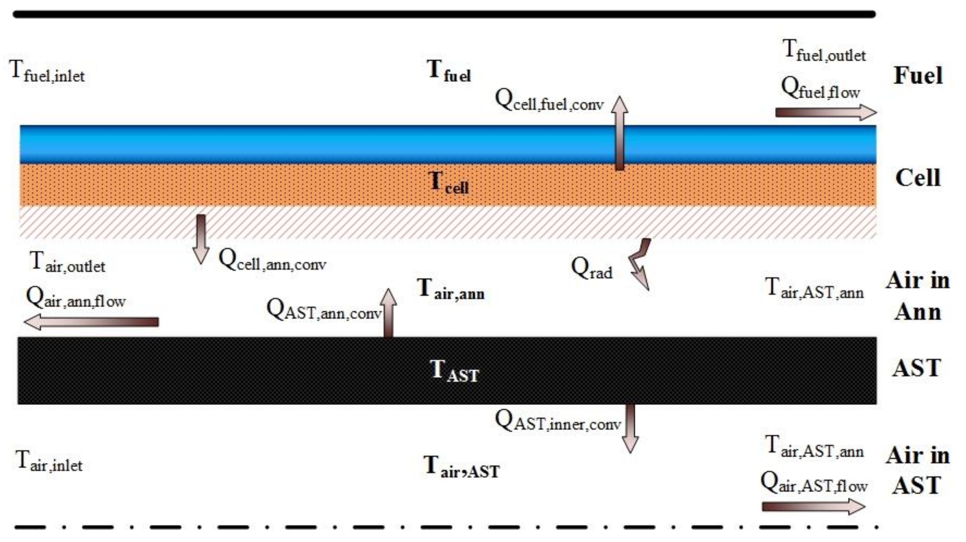
SOFCs are classified into two major types by their geometrical shape, planar, and tubular. Tubular SOFCs are usually appraised to be more superior to the planar ones for their advantages in sealing and structural integrity. However, the two types of SOFCs are equivalent in fundamental principles. Without the loss of generality, a tubular SOFC is chosen to be discussed in this paper. Figure 2 shows the structure of a tubular SOFC. The air (oxidant) is supplied through the air supply tube (AST) into the cell, and then flows past the annular channel of cathode reversely to the fuel, which flows over the anode channel. The electrolyte is sandwiched between the two electrodes.

A reliable dynamic model with proper complexity is essential for the control design of SOFC. Most of the state-of-the-art SOFC papers are based on a benchmark dynamic model that is presented in [22]. This model appears to be very popular in the last decade for its good feasibility for a large scale simulation and its acceptable accuracy on the system dynamics. An important deficiency with the model is that its thermal characteristics are omitted. It has been acknowledged that this simplification is reasonable in studying the dynamics of SOFC since the thermal process is very slow and have little influence on the short-term dynamics. However, the temperature of SOFC is a crucial factor to not only the electrodynamics potential, but also the internal resistance, which are both closely associated with the optimal operation of the SOFC system. Therefore, the benchmark model in [22] is no longer appropriate for the research in this work.

Based on a comprehensive studying of the SOFC’s principles, Wang and Nehrir established a model that includes both the electrochemical and the thermal characteristics of a tubular SOFC [23]. The most significant feature of this model is that it contains detailed mechanism of internal resistance and output voltage. Moreover, with several reasonable assumptions, the heat transfer analysis inside the tube structure is based on the lumped parameter method. These features make the model adequately accurate with reasonable complexity.

3. Steady-State Analysis

Motivated by the dynamic model presented in [23], the analysis of SOFC under steady-state is with the mass conservation, thermal balance and electrochemical properties, respectively based on the following assumptions:

• one-dimensional treatment,
• the air at cathode is with large stoichiometric quantity, and
• the pressure gradient of the gases is uniform along the channels.

The notations in this section are listed in

Table 1. Nomenclature.

Symbol		Superscript/Subscript
A	Area	a	Anode
a, b	Constants with material resistance	act	Activation
E	Electric potential	ann	Annulus
F	Faraday’s constant	AST	Air supply tube
Fu	Fuel utilization	c	Cathode
h	Convective heat-transfer coefficient	cell	Conditions in cell
H	Enthalpy	ch	Conditions in channels
I	Current	chem	Chemical
k	Empirical constant	conv	Convection
M	Mole flow rate	elecyt	Electrolyte.
p	Pressure	flow	Heat carried off by flow
Q	Heat transferred	in/out	Condition of inlet (input)/outlet (output)
T	Temperature	inner/outer	Heat transfer to inner/outer part
V	Voltage	interc	Interconnection between cells
$\epsilon$	Emissivity	ohm	Ohmic
${\xi }_0$, ${\xi }_1$	Coefficients with activation drop	rad	Radiation
$\sigma$	Stefan–Boltzmann constant	*	Effective condition
δ	Length/thickness (m)	H2/O2/H2O	Hydrogen/Oxygen/Water
C	Heat capacity

.

3.1. Mass Conservation

According to Assumption 1, the following equations are obtained:

$$p_{H_2}^{ch}=\frac{p_{H_2}^{in}+p_{H_2}^{out}}{2}$$

(1)

$$p_{O_2}^{ch}=\frac{p_{O_2}^{in}+p_{O_2}^{out}}{2}$$

(2)

$$p_{H_{2}O}^{ch}=\frac{p_{H_{2}O}^{in}+p_{H_{2}O}^{out}}{2}$$

(3)

with Faraday’s Law, the material balance equations for H₂, H₂O, and O₂ in the steady-state are,

$$M_{H_2}^{in}-M_{H_2}^{out}=\frac{I}{2F}$$

(4)

$$M_{H_{2}O}^{in}-M_{H_{2}O}^{out}=-\frac{I}{2F}$$

(5)

$$M_{O_2}^{in}-M_{O_2}^{out}=\frac{I}{4F}$$

(6)

In the flow channels, the following mass flow stands

$$M_a^{out}=M_a^{in}=M_{H_2}^{in}+M_{H_{2}O}^{in}$$

(7)

$$M_c^{out}=M_c^{in}$$

(8)

The mass flows for the gases at outlet of the channels are

$$M_{H_2}^{in}=M_a\frac{p_{H_2}^{in}}{p_a^{in}},M_{H_2}^{out}=M_a\frac{p_{H_2}^{out}}{p_a^{out}}$$

(9)

$$M_{H_{2}O}^{in}=M_a\frac{p_{H_{2}O}^{in}}{p_a^{in}},M_{H_{2}O}^{out}=M_a\frac{p_{H_{2}O}^{out}}{p_a^{out}}$$

(10)

$$M_{O_2}^{in}=M_c\frac{p_{O_2}^{in}}{p_c^{in}},M_{O_2}^{out}=M_c\frac{p_{O_2}^{out}}{p_c^{out}}$$

(11)

The fuel utilization is defined by

$$F_u=\frac{I}{2F}/M_{H_2}^{in}.$$

(12)

3.2. Thermal Balance

The chemical reaction in a SOFC is carried out in the electrode-electrolyte tier (EET) with the production of heat. The electrode-electrolyte tier is cooled by the fuel and air flows through the channel. In the meanwhile, some of the heat transfers to the air supply tube by means of radiation. A cross-sectional profile of a tubular SOFC and the heat transfer are shown in Figure 3. Note that only half of the profile is drawn here because of the symmetry of the profile.

The heat transfer analysis is based on the lumped parameter method. Five lumps are considered here, which are the fuel in the channel, the electrode-electrolyte tier, the air in the annulus, the air supply tube, and the air inside the tube, respectively, from top to bottom in the figure. In the manner of lumped parameter systems, the temperature difference inside each lump is neglected. With the lumped parameter method, the average value of the temperature at two ends is used to represent the gas temperature in the channels:

$$T_{air,AST}=\frac{T_{air,inlet}+T_{air,AST,ann}}{2}$$

(13)

$$T_{air,ann}=\frac{T_{air,AST,ann}+T_{air,outlet}}{2}$$

(14)

$$T_{fuel}=\frac{T_{fuel,inlet}+T_{fuel,outlet}}{2}$$

(15)

The Cell Tube:

For the EET, in steady-state the heat produced is completely dissipated in different ways. The following equation stands in this case:

$$Q_{chem}-V_{out}\cdot I=Q_{rad}+Q_{cell,ann,conv}+Q_{cell,fuel,conv}$$

(16)

The left hand side of the equation is the heat production in the cell, which is the difference between the total chemical energy that is released by the reactant and the actual electrical power output. The right hand side is the heat transfer with the cell in different ways. The heat transfer with other parts of the cell is listed as follows.

The fuel:

$$Q_{fuel,flow}=Q_{cell,fuel,conv}$$

(17)

Air between cell and AST:

$$Q_{air,ann,flow}=Q_{cell,ann,conv}+Q_{AST,ann,conv}$$

(18)

AST:

$$Q_{rad}=Q_{AST,inner,conv}+Q_{AST,ann,conv}$$

(19)

Air in AST:

$$Q_{air,AST,flow}=Q_{AST,inside,conv}$$

(20)

The heat transfer terms in (16) ~ (20) are calculated through heat transfer equations as:

$$Q_{chem}=n_{H_2,consumed}\cdot \Delta H=\frac{I}{2F}\cdot \Delta H$$

(21)

$$Q_{rad}={\epsilon }_{AST}^{*}\sigma A_{AST,outer}(T_{cell}^4-T_{AST}^4)$$

(22)

$$Q_{cell,ann,conv}=h_{cell}{A}_{cell,inner}(T_{cell}-T_{air,ann})$$

(23)

$$Q_{cell,fuel,conv}=h_{cell}{A}_{cell,outer}(T_{cell}-T_{fuel})$$

(24)

$$Q_{\mathrm{AST},\mathrm{ann},\mathrm{conv}}=h_{AST,outer}{A}_{AST,outer}(T_{air,cell}-T_{AST})$$

(25)

$$Q_{AST,inner,conv}=h_{AST,inner}{A}_{AST,inner}(T_{AST}-T_{air,AST})$$

(26)

$$Q_{air,ann,flow}=M_c{M}_{mw,air}{C}_{air}(T_{air,outlet}-T_{air,AST,ann})$$

(27)

$$Q_{air,AST,flow}=M_c{M}_{mw,air}{C}_{air}(T_{air,AST,ann}-T_{air,inlet})$$

(28)

$$\begin{array}{l}{Q}_{fuel,flow}=Q_{H_2,flow}+Q_{H_{2}O,flow}\\ Q_{H_2,flow}=(M_{H_2}^{in}+M_{H_2}^{out})(T_{fuel}^{out}-T_{fuel}^{in})C_{H_2}{M}_{mw,H_2}\\ Q_{H_{2}O,flow}=(M_{H_{2}O}^{in}+M_{H_{2}O}^{out})(T_{fuel}^{out}-T_{fuel}^{in})C_{H_{2}O}{M}_{mw,H_{2}O}\end{array}$$

(29)

3.3. The Electrochemical Relations

The potential of fuel cells is subject to the Nernst equation:

$$E_{cell}=E_{0,cell}^0-k_E(T-298)+\frac{RT}{4F}\ln \left[\frac{{(p_{H_2}^{*})}^2{p}_{O_2}^{*}}{{(p_{H_{2}O}^{*})}^2}\right]$$

(30)

where, $E_{0,cell}^0$ is the standard electrode potential, the value of which depends on the species of reactant. For the reaction in SOFC, the reference potential is 1.229 V. $E_{cell}$ is actually the open-circuit voltage of the fuel cell. For a SOFC with electrical loads, the output voltage is less than the $E_{cell}$ due to the varieties of voltage drop including activation drop, ohmic resistance drop, and concentration drop. Therefore, the actual output voltage is calculated as

$$V_{cell}=E_{cell}-V_{act,cell}-V_{ohm,cell}-V_{conc,cell}$$

(31)

The voltage drops are calculated as [23]:

$$V_{conc,cell}=\frac{RT}{4F}\left\{\ln \left[\frac{{(p_{H_2}^{ch})}^2{p}_{O_2}^{ch}}{{(p_{H_{2}O}^{ch})}^2}\right]-\ln \left[\frac{{(p_{H_2}^{*})}^2{p}_{O_2}^{*}}{{(p_{H_{2}O}^{*})}^2}\right]\right\}$$

(32)

$$V_{act,cell}={\xi }_0+{\xi }_{1}T+\frac{2RT}{zF}{\sinh }^{-1}(\frac{I}{2I_0})$$

(33)

$$V_{ohm,cell}=\frac{a_{elecyt}\exp (b_{elecyt}/T)}{A_{cell}}{\delta }_{elecyt}+\frac{a_{\mathrm{int}erc}\exp (b_{\mathrm{int}erc}/T)}{A_{cell}}{\delta }_{\mathrm{int}erc}$$

(34)

Note that the model presented above is for single cell. Since the electric potential provided by the electrochemical reaction in a single fuel cell is very small, numbers of the fuel cells are usually cascaded together (referred to as fuel cell stacks) to acquire a proper voltage level in the practical application.

4. Control System Design

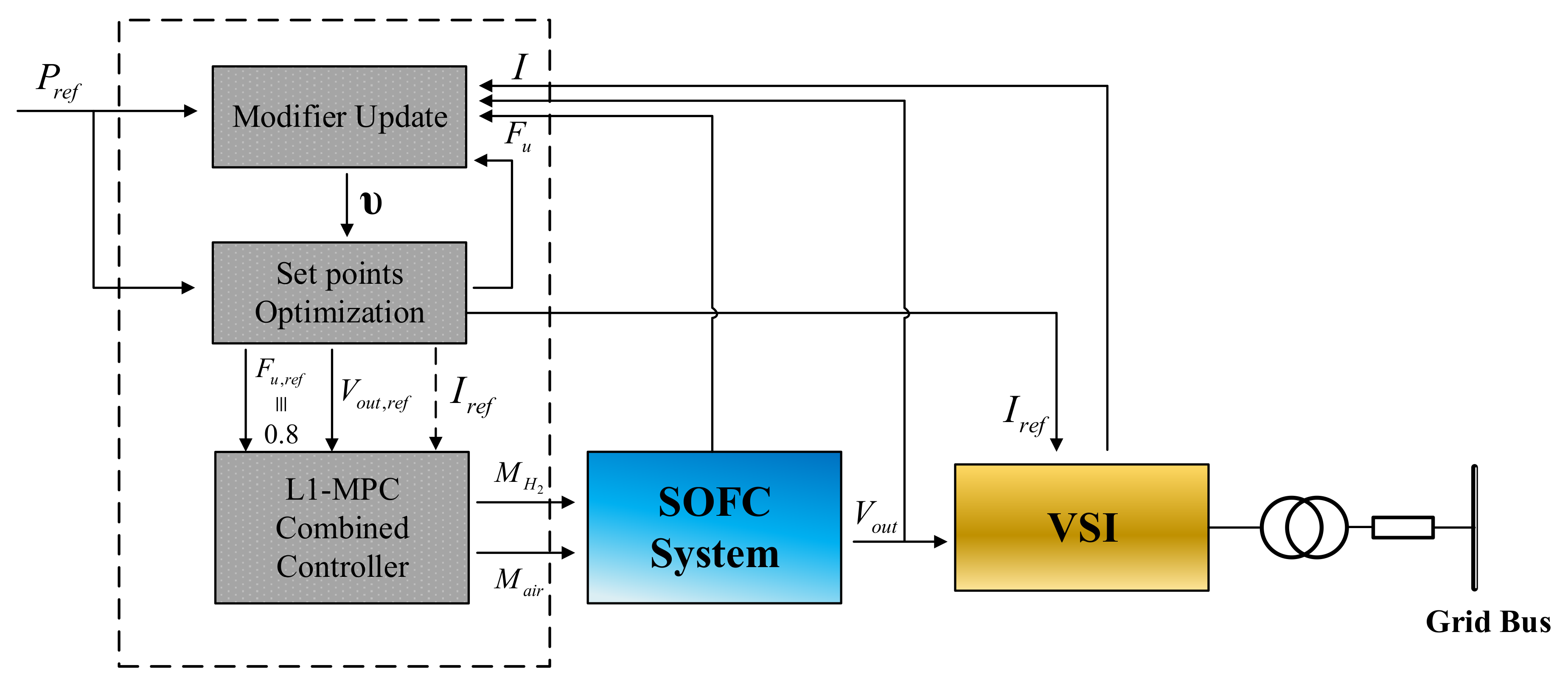
The total control strategy in this work is proposed to have a hierarchical architecture, with which the control system is generally divided into a supervisory level in the upper and an underlying level in the lower, as shown in Figure 4.

In the upper level is a set point (SP) scheduler. The scheduler receives unit load demand from the power grid dispatching system. With the unit load demand, online optimizations are carried out by the SP scheduler with the steady-state model of the fuel cell to find a set of target for voltage and current under which the corresponding steady states of the SOFCs satisfies the load demand with optimal economic performance. To deal with the mismatch between the steady-state model and the real plant, a modification mechanism will be working with the SP scheduler to make the acquired target as precise as possible.

In the lower level, a SOFC controller is working with a voltage source inverter (VSI). With the set point for voltage being provided from the SP scheduler, the SOFC controller steers the SOFC’s output voltage to the set point by manipulating the inlet fuel flow to the anode and the inlet air flow to the cathode. At the same time, the fuel utilization should be maintained within the tolerant range (0.7 to 0.9) in transient states and be driven to the proper value (0.8) in steady states. For this purpose, a combined L1-MPC controller is put forward to generate the control signal for the manipulated fuel and air flows, handling the nonlinear dynamics in the SOFCs and taking care of the system constraints with acceptable online computation. The cooperating VSI is integrated with its own controller. The task for the VSI is to control the current flow to the power grid. 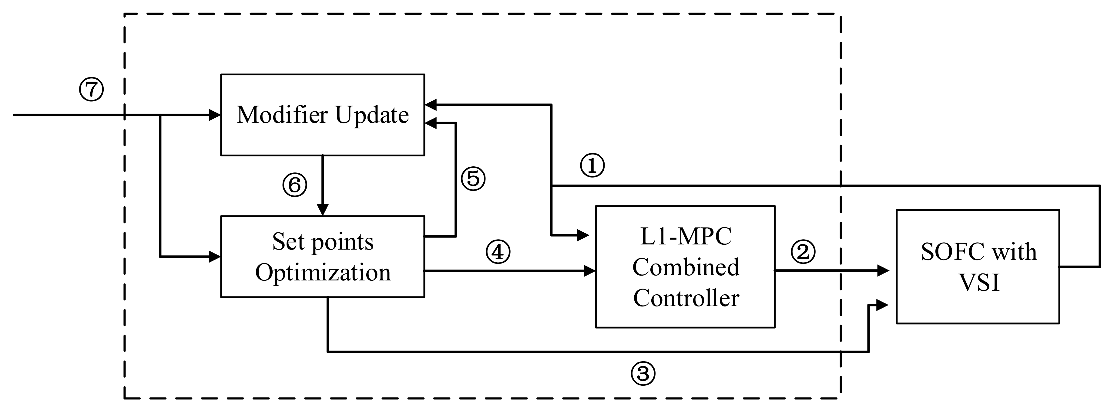The specific control algorithm of VSI is out of the scope of this paper and will not be discussed here, but it is worth pointing out that the time constant of the VSI’s dynamics (around 0.1 s) is much smaller than that of the SOFC’s to a new steady state [24]. Therefore, the transient process of the VSI will not be considered in the SOFC controller design. The algorithm discussed in detail for the SOFC controller will only include the upper level set point scheduler with modifier and the level layer L1-MPC combined controller (as marked with dashed box in Figure 4). This part is redrawn in Figure 5 with the signal flow components listed in

Table 2. The components of signal flow in designed control scheme.

Number	Signal	Number	Signal
1	I, Vout, Fu	5	Optimization results
2	MH2, Mair	6	Modifier term υ
3	Iref	7	Pref
4	Fu,ref, Vout,ref, Iref	-	-

. The specifics of the L1-MPC controller will be discussed in this section.

4.1. Set Point Scheduler

In the supervisory level, the set points of current and output voltage is acquired from an online nonlinear optimization module using the steady-state model given by (1)~(34), and the unit load demand given by the grid dispatching system. With the unit load demand, the working condition of SOFC satisfies

$$I_{ref}\cdot V_{out,ref}=P_{ref}$$

(35)

and the proper fuel utilization

$$F_{u,ref}=0.8$$

(36)

The goal of the optimization considered in this work is to minimize the internal power dissipation of the SOFC under given output power. With the notations that $y_s={\left[V_{out},I\right]}^T$, $x_s={\left[p_{H_2}^{ch},p_{H_{2}O}^{ch},p_{O_2}^{ch},T_{fuel},T_{air,cell},T_{cell},T_{air,AST},T_{AST}\right]}^T$, $u_s={\left[M_{air},M_{H_2}\right]}^T$, the mathematical formulation of the optimization problem is

$$\begin{array}{c}\left[y_{ref}(k),x_{ref}(k),u_{ref}(k)\right]=arg \underset{y_s,x_s,u_s}{\min }(q_{chem}-I\cdot V_{out})\\ \begin{array}{cc}s.t.& \mathsf{\Phi }(y_s,x_s,u_s)=0\end{array}\end{array}$$

(37)

where $\mathsf{\Phi }(y_s,x_s,u_s)=0$ is the equality constraint constituted by the steady-state model in Section 3. The acquired $V_{out,ref}$ are given to the combined L1-MPC controller together with the expected fuel utilization $F_{u,ref}$ for the regulation of the SOFC, while $I_{ref}$ is fed to the VSI to adjust the output current of the SOFC. For practical SOFC systems, the optimal operation cannot be achieved by simply solving (37) due to the model errors. The model errors come from the structure mismatch during modeling and parameter perturbation during operation. Since the model errors are not avoidable, the nominal solution of (37) is never likely to be optimal in reality. To deal with this problem, an approach used in earlier time is to re-identify the parameters online using the plant measurements in steady states. The approach is now referred as “two-step approach” in the literatures [25]. However, the two-step approach is usually not effective in practice as the parameter identification is easy to converge to a local optimization. Another approach is to solve the optimization problem with a modifier, which is substantially a lumped estimation of model errors, added to the constraints to correct the model values [26]. Owing to the avoidance of complex identification and the ability of acquiring an acceptable optimization result in practice, the modifier approach is now widely used in so-called real-time optimization in industry and it is applied in the SOFCs discussed in this paper.

The amendatory optimization problem with modifier is formulated as:

$$\begin{array}{l}{y}_{ref}(k)=arg \underset{y,x,u}{\min }(q_{chem}-I\cdot V_{out})\\ \begin{array}{cc}s.t.& \mathsf{\Phi }(y_s,x_s,u_s)=\upsilon (k)\end{array}\end{array}$$

(38)

where $\upsilon (k)$ denotes the modifier, which is updated with

$$\upsilon (k)=\frac{1}{K_{\upsilon }+1}\upsilon (k-1)+\frac{K_{\upsilon }}{K_{\upsilon }+1}[\mathsf{\Phi }(y_s(k),x_s(k),u_s(k))-\mathsf{\Phi }(y_{ref}(k-1),x_{ref}(k-1),u_{ref}(k-1))]$$

(39)

where $K_{\upsilon }$ is a designed parameter that determines the convergence rate of modifier $\upsilon$. Notice that the elements in vector $x$ are internal states of SOFC and are difficult to measure. In this case, we replace $x(k)$ with $x_{ref}(k-1)$ and attribute the corresponding error to the lumped modifier $\upsilon (k)$.

Before modifier updating, steady-state detection should be conducted to capture the input/output data used for modifier updating. The steady-state detection used to be a much studied topic in process control in the late 20th century and many approaches have been introduced in that period (see [27,28,29]). For gird-connected SOFCs participating in peaking regulation, the output power should change frequently in order to compensate the power deficit induced by intermittent energy sources. In this case, the system will operate at non-steady states for most of the time. In consideration of this characteristics, we apply a method that is given by Cao and Rhinehart [29]. The applied approach provided a way to simply use a sequence of filtered data, preventing the requirement for considerable data storage and user expertise. Denoting $X$ as the indicator variable that is used to detect the steady state, the procedure for steady-state detection is carried out iteratively as follows:

Step 1: Calculate a first-order filtered term of $X$ by:

$$X_{f_i}={\lambda }_1{X}_i+(1-{\lambda }_1)X_{f_{i-1}}$$

(40)

Step 2: An estimation of mean square deviation is calculated by:

$${\nu }_{f,i}^2={\lambda }_2{(X_i-X_{f_{i-1}})}^2+(1-{\lambda }_2){\nu }_{f,i-1}^2$$

(41)

Step 3: Use the following equation to get estimation to the squared differences of successive data:

$${\delta }_{f,i}^2={\lambda }_3{(X_i-X_{i-1})}^2+(1-{\lambda }_3){\delta }_{f,i-1}^2$$

(42)

Step 4: Taking the ratio of the two estimates determined by (41) and (42):

$$R_i=\frac{(2-{\lambda }_1){\nu }_{f,i}^2}{{\delta }_{f,i}^2}$$

(43)

In the equations above ${\lambda }_1$, ${\lambda }_2$, ${\lambda }_3$ are parameters that satisfy $0<{\lambda }_1,{\lambda }_2,{\lambda }_3\le 1$. The criterion for steady state is $\left|R_i-1\right|\le \alpha$, where $\alpha$ is a chosen threshold value for the judgment of steady states.

In this work, the output power is chosen as the indicator for steady-state. The reason is that the output power is determined by both the current and voltage. Further, the voltage is determined simultaneously by a large amount of the SOFC parameters, thus it is sensitive to the unsteadiness of the system dynamic. In this sense, the output power might be the most comprehensive and a reliable variable to indicate the achievement of steady states.

When a steady state is detected, the modifier update mechanism with (39) is conducted using corresponding input and output data of the system. The steady state detection procedure can be deployed in an individual module separate to the set point scheduler with higher sampling frequency, or integrated with the set point scheduler. The whole control scheme with the modifier is presented in Figure 4.

4.2. Combined L1-MPC Controller

For SOFC tracking controller design, the outputs and inputs of the control problem are denoted as y = [y₁,y₂]^T = [V_out,F_u]^T and u = [u₁,u₂]^T = [M_H2,M_air]^T, respectively. Then, the controlled system is considered as:

$$y(s)=G(s)\cdot u(s)+\delta (s)$$

(44)

where $G(s)$ is a 2 × 2 transfer function matrix, $\delta (s)$ denotes the lumped uncertainty terms, which contains all of the nonlinearity associated with the system, and (s) denote systems, variables, or signals in the s-domain with Laplace transformation.

The system (44) can be rewritten as,

$$y_i(s)=G_{ii}(s)(u_i(s)+{\sigma }_i(s))+{\displaystyle {\sum }_{j=1,j\ne i}^n{G}_{ij}(s)u_j(s)}$$

(45)

where for i = 1, 2, where $G_{ii}(s)$ denotes the (i,i)-th element of $G(s)$, ${\sigma }_i(s)$ is generalized uncertainty term that satisfies,

$$G_{ii}(s){\sigma }_i(s)={\delta }_i(s)$$

(46)

for i = 1, 2, and ${\delta }_i(s)$ denotes the i-th element of $\delta (s)$.

The corresponding time-domain form of ${\sigma }_i(s)$, $\sigma (t)$ can be written as,

$$\sigma (t)=f(y(t),t)$$

(47)

The discussion is based on the following assumptions:

1. The diagonal elements of transfer function matrix $G(s)$ are positive real transfer functions.

2. There exist constants $L>0$ and $L_0>0$, possibly arbitrarily large, such that

$$\left|f(t,y)-f(t,\stackrel{⌢}{y})\right|\le L\left|y-\stackrel{⌢}{y}\right|,\left|f(0,y)\right|\le L\left|y\right|+L_0$$

(48)

hold uniformly in t.

3. The variation rate of $\sigma (t)$ is bounded,

$$\left|\dot{\sigma }(t)\right|\le d_{\sigma }$$

(49)

Then, it follows from the basic procedure of L1 adaptive controller, the following output predictor is constructed:

$${\widehat{y}}_i(s)=G_{ii}(s)(u_i(s)+{\widehat{\sigma }}_i(s))+{\displaystyle {\sum }_{j=1,j\ne i}^n{G}_{ij}(s)u_j(s)}$$

(50)

for i = 1, 2, where $G_{ii}(s)$ denotes the (i,i)-th element of $G(s)$, and ${\widehat{\sigma }}_i(s)$ is the Laplace form of the estimation ${\widehat{\sigma }}_i(t)$, which is updated by the adaptation law:

$${\dot{\widehat{\sigma }}}_i(t)=\mathsf{\Gamma }Proj({\widehat{\sigma }}_i,-sign(g_{ii}){\tilde{y}}_i)$$

(51)

where Proj represents the projection operator [21], ${\tilde{y}}_i={\widehat{y}}_i-y_i$, $g_{ii}$ is the DC gain of the i-th diagonal element in $G(s)$, $\mathsf{\Gamma }$ is the adaptive gain. Then, the control law is presented as

$$u_i=u_{L_1,i}+u_{MPC,i}$$

(52)

$$u_{L_1,i}=-C_i(s)\cdot {\widehat{\sigma }}_i(s)-{\displaystyle {\sum }_{j=1,j\ne i}^n\frac{G_{ij}(s)}{G_{ii}(s)}{u}_{L_1,j}}(s)$$

(53)

where $C_i(s)$ is low pass filters with unit DC gain satisfying

$${\Vert G_{ii}(s)\cdot (1-C_i(s))\Vert }_{L_1}{l}_i<1,$$

(54)

$u_{MPC}$ is the MPC control component

$$u_{MPC}(t)=u^{*}(k{T}_{MPC}),t\in [k{T}_{MPC},(k+1)T_{MPC}),$$

(55)

such that $u^{*}(k{T}_{MPC})$ is from the solution of the following optimization problem:

$$\begin{array}{l}\min J={\displaystyle \sum _{i=1}^N({\Vert y(k+i|k)-y_{ref}\Vert }_Q^2+{\Vert u(k+i-1|k)-{\mu }_{ref}\Vert }_R^2})\\ s.t. y(k+i|k)=cx(k+i|k)\\ x(k+i|k)=Ax(k+i-1|k)+Bu(k+i-1|k)\\ u_{\min }-u_{L_1}(k)\le u(k+i|k)\le u_{\max }-u_{L_1}(k)\\ y_{\min }\le y(k+i|k)\le y_{\max }\\ x(k|k)=\widehat{x}(k)\\ \widehat{x}(k)=A\widehat{x}(k-1)+Bu(k-1)+L(c\widehat{x}(k-1)-y(k-1))\end{array}$$

(56)

where A, B, and c, are the system matrices of discrete state-space model corresponding to $G(s)$ with sampling time $T_{MPC}$, $u_{\min }$, and $u_{\max }$ are the input constraints, $y_{\min }$ and $y_{\max }$ are the expected output constraints, ${\mu }_{ref}$ is a reference input corresponding to the output reference $y_{ref}$ with the linear model (A, B, c) calculated by ${\mu }_{ref}={(c{(I-A)}^{-1}B)}^{-1}{y}_{ref}$, $u_{L_1}(k)$ is the L1 adaptive term at the sample time k, $y(k-1)$ denotes the measurement of y at the last sample, $L$ is a matrix that keep all of the eigenvalues of matrix $(\overline{A}+L\cdot \overline{c})$ inside the unit circle.

Equation (56) is a standard formulation for output feedback MPC with a state observer and can be easily transformed to a quadratic programming (QP) with a few steps of algebraic operation as follows.

The first two equations of (56) makes the prediction of the system output:

$$\begin{array}{l}y(k+1|k)=c(Ax(k|k)+Bu(k|k))\\ y(k+2|k)=c(A^{2}x(k|k)+ABu(k|k)+Bu(k+1|k))\\ ⋮\\ y(k+M|k)=c(A^{M-1}x(k|k)+Bu(k+M-1|k)+ABu(k+M-2|k)+\cdots \\ +A^{M-1}Bu(k|k))\\ ⋮\\ y(k+N|k)=c(A^{N}x(k|k)+A^{M-1}Bu(k|k)+A^{M-2}Bu(k|k)+\cdots \\ +(B+AB+\cdots +A^{N-M}B)u(k+M-1|k))\end{array}$$

(57)

In (57), M is a tunable parameter called controlled horizon in MPC theory, with which, the predicted system input u (k + i|k) keeps invariant when i ≥ M. Then, the optimization problem (56) can be transformed to the following QP form with (57):

$$\begin{array}{l}\underset{\mathit{U}(k)}{\min } {\mathit{U}}^T(k)(G_y^T\mathit{Q}{G}_y^T+\mathit{R}){\mathit{U}}^T(k)+2(x^T(k|k)F_y^T\mathit{Q}{G}_y-Y_{ref}^T\mathit{Q}{G}_y-U_{ref}^T\mathit{R})\mathit{U}(k)\\ s.t. {\mathit{U}}_{\min }(k)\le \mathit{U}(k)\le {\mathit{U}}_{\max }(k)\\ {\mathit{Y}}_{\min }-F_{y}x(k|k)\le G_y\mathit{U}(k)\le {\mathit{Y}}_{\max }-F_y(k|k)\end{array}$$

(58)

where,

$$\begin{array}{c}{G}_y=\left[\begin{array}{ccc}cB& 0& 0\\ ⋮& \ddots & 0\\ c{A}^{M-1}B& \cdots & cB\\ ⋮& & ⋮\\ c{A}^{N-1}B& \cdots & {\displaystyle \sum _{i=1}^{N-M+1}c{A}^{i-1}B}\end{array}\right],F_y=\left[\begin{array}{c}cA\\ ⋮\\ c{A}^N\end{array}\right],\mathit{Q}=\left[\begin{array}{ccc}Q& & \\ & \ddots & \\ & & Q\end{array}\right],\\ R=\left[\begin{array}{ccc}R& & \\ & \ddots & \\ & & R\end{array}\right]\\ \mathit{U}(k)=\left[\begin{array}{c}u(k|k)\\ u(k+1|k)\\ ⋮\\ u(k+M|k)\end{array}\right],{\mathit{U}}_{\min }=\left[\begin{array}{c}{u}_{\min }-u_{L_1}(k)\\ ⋮\\ u_{\min }-u_{L_1}(k)\end{array}\right],{\mathit{U}}_{\max }=\left[\begin{array}{c}{u}_{\max }-u_{L_1}(k)\\ ⋮\\ u_{\max }-u_{L_1}(k)\end{array}\right],\hfill \\ {\mathit{Y}}_{\min }=\left[\begin{array}{c}{y}_{\min }\\ ⋮\\ y_{\min }\end{array}\right],{\mathit{Y}}_{\max }=\left[\begin{array}{c}{y}_{\max }\\ ⋮\\ y_{\max }\end{array}\right],\hfill \end{array}$$

Note that to avoid the FU from exceeding the upper limit and triggering fuel protection, the lower bound for fuel flow (u₁) should be updated at each sampling time with the reference current at the moment:

$$u_{1,\min }=\frac{I_{ref}}{2F\cdot F_u^{upper}}$$

(59)

where $F_u^{upper}$ is the upper limit for FU and is usually set to be 0.9 or is slightly lower than 0.9 for safety.

The optimization problem (56) is solved online at each sampling time with the receding horizon framework. In this manner, the first term of the solution sequence U(k) is applied on the system, i.e.,

$$u^{*}(k{T}_{MPC})=u(k|k)$$

(60)

Theorem 1.

For plant (44) applied with control law in (52), and defining a reference system as

$$y_{ref,i}(s)=G_{ii}(s)(u_{ref,i}(s)+{\sigma }_{ref,i}(s))+{\displaystyle {\sum }_{j=1}^n{G}_{ij}(s)u_{ref,j}}(s)$$

(61)

with control input

$$u_{ref,i}=u_{L_1,ref,i}+u_{MPC,i}$$

(62)

$$u_{L_1,ref,i}=-C_i(s)\cdot {\sigma }_{ref,i}(s)-{\displaystyle {\sum }_{j=1,j\ne i}^n\frac{G_{ij}(s)}{G_{ii}(s)}{u}_{L_{1}ref,j}}(s)$$

(63)

Then, the following bound of system transient performance holds:

$${\Vert y_i-y_{ref,i}\Vert }_{L_{\infty }}\le \frac{{\Vert C_i(s)\Vert }_{L_1}}{1-{\Vert G_{ii}(s)\cdot (1-C_i(s))\Vert }_{L_1}}\sqrt{\frac{{\theta }_{m,i}}{{\lambda }_{\min }(P_i)\mathsf{\Gamma }}}$$

(64)

where ${\theta }_{m,i}=4{\sigma }_{b,i}^2+4\frac{{\lambda }_{\max }(P_i)}{{\lambda }_{\min }(Q_i)}{\sigma }_{b,i}{d}_{\sigma ,i}$, $P_i$, $Q_i$ are positive definite matrices, ${\sigma }_{b,i}$ is estimated maximum value for ${\sigma }_i(t)$, ${\lambda }_{\max }(\cdot )$ and ${\lambda }_{\min }(\cdot )$ respectively denote the maximum and minimum eigenvalue of a matrix, and $d_{\sigma ,i}$ is defined with (49).

Remark 1.

Defining the following ideal system with no uncertainties:

$$\overline{y}(s)=G(s)\cdot u_{MPC}(s)$$

(65)

The difference between the output of ideal system (65) and the output of the reference system (58) satisfies

$$\delta y_i(s)={\overline{y}}_i(s)-y_{ref,i}(s)=G_{ii}(s)(1-C_i(s)){\sigma }_{ref,i}(s)$$

(66)

Note that $\delta y_i(s)$ is a result of ${\sigma }_{ref,i}(s)$ filtered by the low-pass system $G_{ii}(s)$ cascading with high-pass filter $1-C_i(s)$. So, if the cut-off frequency of the high-pass filter is much larger than the bandwidth of the low-pass system $G_{ii}(s)$, the cascaded system will result in a no-pass filter and we get $\delta y_i(s)\to 0$. Thus, it is reasonable to make the approximation that $y\approx y_{ref}\approx \overline{y}$.

4.3. Fuel Starvation Protection

It is very important to point out that the protection constraint imposed in the MPC still cannot guarantee the avoidance of fuel starvation for the following two reasons:

1. Since the sampling time of MPC is usually much longer than the time-scale of power electronic devices. If the unit load demand changes during the interval of two MPC sampling point, MPC may not be able to respond in time before the fuel starvation occurs.

2. Since the action of the valves usually takes seconds, the supplementary fuel lags the instantaneous consumption caused by the leap of the current.

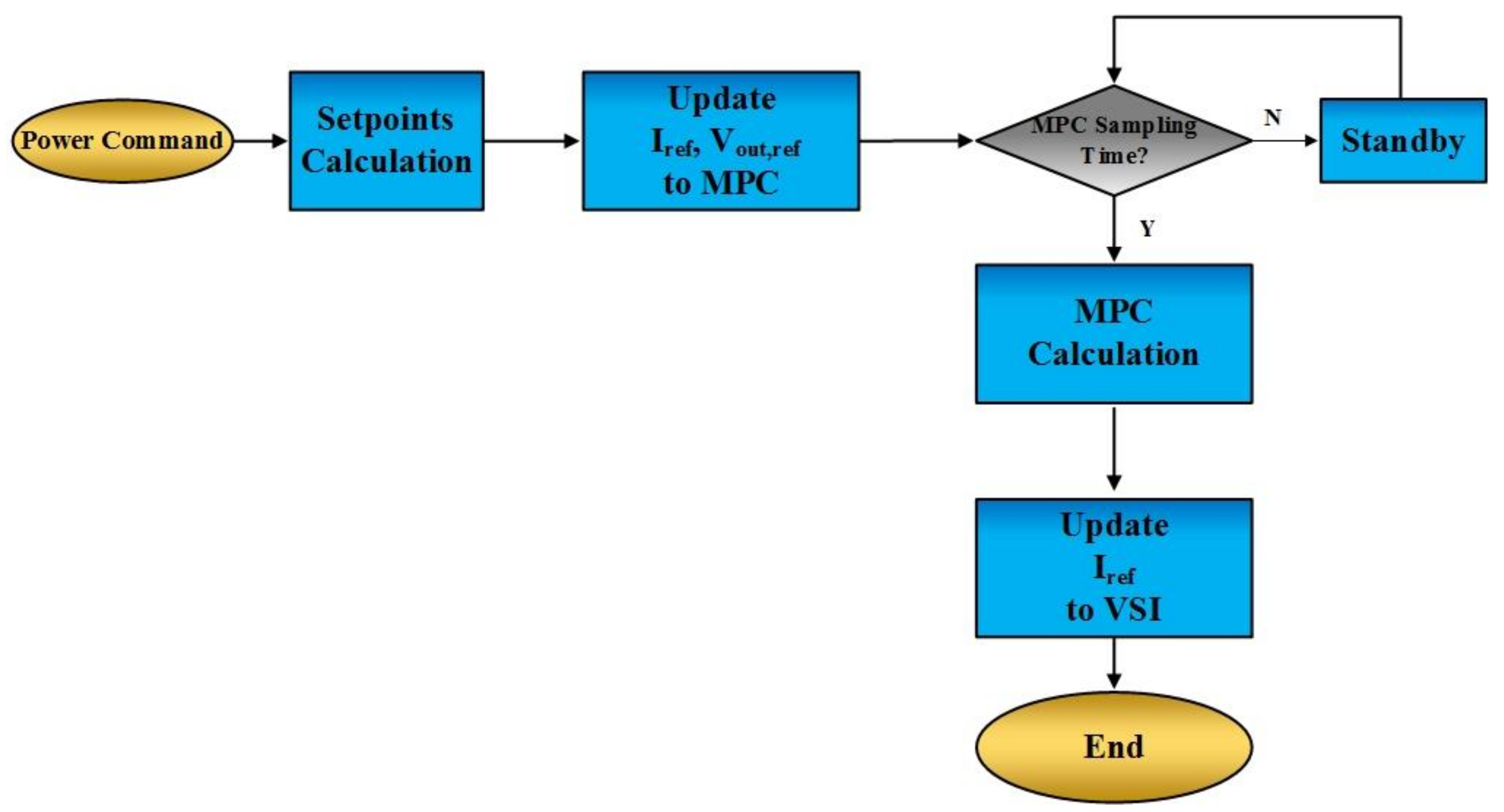
To overcome the first defect, protection logic, as shown in Figure 6, is added to the control system. When the supervisory level produces a new reference current, the current value will be hold in the memory until the next sampling time of MPC. Additionally, a load governor, which is designed as a first-order filter to smooth the current reference is transmitted to the converter system.

5. Simulation Results

The simulation is conducted on the model introduced in Section 3 with Matlab/Simulink^TM with the configuration of a 5 kw SOFC stack. The SOFC stack is composed of 192 cascading basic fuel cells. Without a loss of generality, the simulation is conducted on a single cell. However, the experimental data is amplified by the cell number in the figures drawing for better exhibition.

Firstly, open loop step response experiments are conducted in order to obtain a locally linearized dynamic model of SOFC. The open loop experiment is conducted with an initial state of V_out = 170.0 (V) and I = 20 (A), which implies that P = 3400 (W). The corresponding flows of H₂ and Air for each cell are M_H2 = 0.15 × 10⁻⁴ mol/s, M_air = 0.5 × 10⁻⁴ mol/s. Making M_H2 step up from 0.15 × 10⁻⁴ mol/s by 20% and M_air step up from 0.5 × 10⁻⁴ mol/s by 20%, respectively, four data sets of input-output pairs are collected. Then, the linear locally linearized dynamic model in the form of $2\times 2$ transfer function matrix is acquired by identification with the step response experiment data at the initial sate.

$$G(s)=\left[\begin{array}{cc}\frac{28.51}{s+0.0834}& \frac{1.098}{s+0.08753}\\ \frac{-378}{s+0.09847}& \frac{1.539e-06}{s+0.09847}\end{array}\right]$$

The parameters for L1-MPC controller are:

$$\begin{array}{c}\mathsf{\Gamma }{=1\mathrm{e}}^5,C_1(s)=1/(s+1),C_2(s)=0.4/(s+0.4),Q=diag(0.5,10),\\ R=diag(100,100),N=50,M=5,L={\left[\begin{array}{ccc}0.0329& -0.0095& 0\\ 0& 0& -0.0058\end{array}\right]}^T,\\ y_{\min }={\left[\begin{array}{cc}0.5& 0.72\end{array}\right]}^T,y_{\max }={\left[\begin{array}{cc}1.5& 0.88\end{array}\right]}^T,u_{\min }={\left[\begin{array}{cc}1.0\mathrm{e}-4& 1.0\mathrm{e}-4\end{array}\right]}^T,\\ u_{\max }={\left[\begin{array}{cc}2.55\mathrm{e}-3& 24.5\mathrm{e}-3\end{array}\right]}^T.\end{array}$$

The sampling time of Modifier, set points (SP) scheduler and L1-MPC controller are set to be 1 s, 10 s and 10 s, respectively. The parameters of inlet air and fuel are assumed to keep constant during the simulation:

$$p_a^{in}=p_c^{in}=2atm,T_{air,inlet}=T_{fuel,inlet}=973K$$

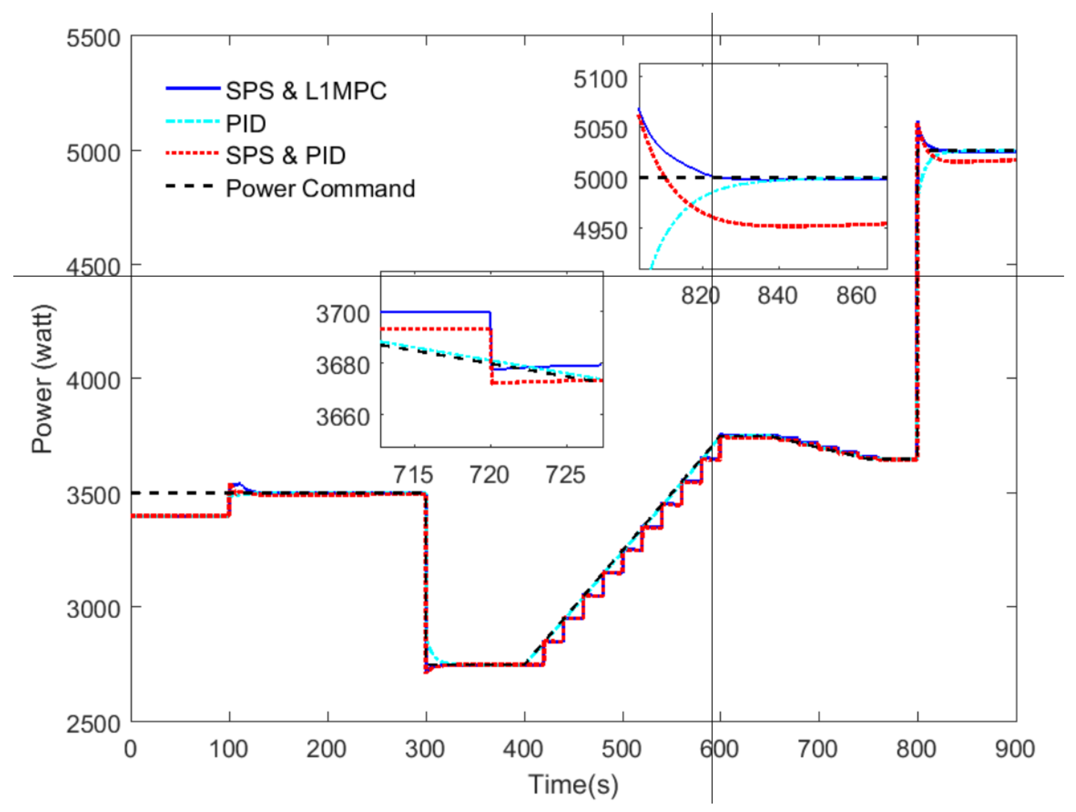
The initial power command is P_ref = 3500 W. At t = 100 s, switch the whole control system on. At t = 300 s, the unit load demand steps to P_ref = 2750 W, and it then starts ramping at t = 400 s by 5 W/s to P_ref = 3750 W. Beginning at 650 s, P_ref ramps to 3650 W by 1 W/s. Finally, P_ref steps to 5000 W at t = 800 s.

To further exhibit the advantage of the proposed control strategy, comparative experiments are designed with conventional control strategies based on proportional-integral-derivative (PID) controller designs.

First, a SOFC system operating with no set point scheduler is tested. Since PID is an error-based control algorithm that needs specific set point to work with, in the case with no set point scheduler, different control architecture have to be applied with the SOFC to make the output power tracking the unit load demand. In consideration of the SISO feature of PID, an alternative architecture is to use a PID controller directly control the output power by producing the reference current for the VSI. Another PID controller is applied to control the fuel utilization by manipulating the inlet fuel flow. Meanwhile, make the inlet air flow invariant. This compared control architecture is presented in Figure 7.

Another comparison is to use the set point scheduler to produce the set point for output voltage and current, while for the SOFC, two PID controllers are employed. One is to control the FU by manipulating the inlet fuel flow and the other is for SOFC system to control the voltage by manipulating the inlet air flow.

The output power of the SOFCs under proposed control strategy and two comparative ones is shown in Figure 8. It is obvious that, although the three systems all have the ability to track the unit load demand on some level, the system with proposed SP scheduler and L1-MPC controller has the best tracking performance. The one with SP scheduler and PID controller have a fairly good tracking performance in the first period. However, at the end of the simulation time, that is, with power command of 5000 KW, the output power has large disparity to the unit load demand. It can be seen from the tendency that it needs a long time to eliminate the residual error. This can be attributed to the weakness of PID controller to handle the SOFC’s nonlinearities in the high power zone.

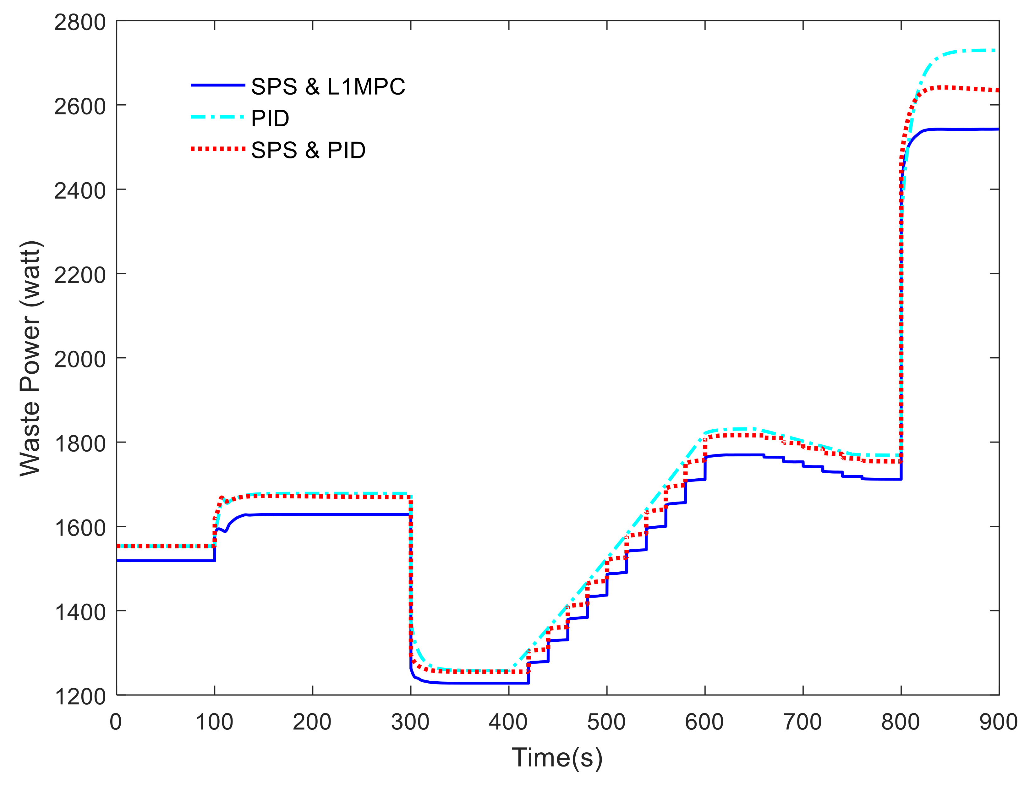
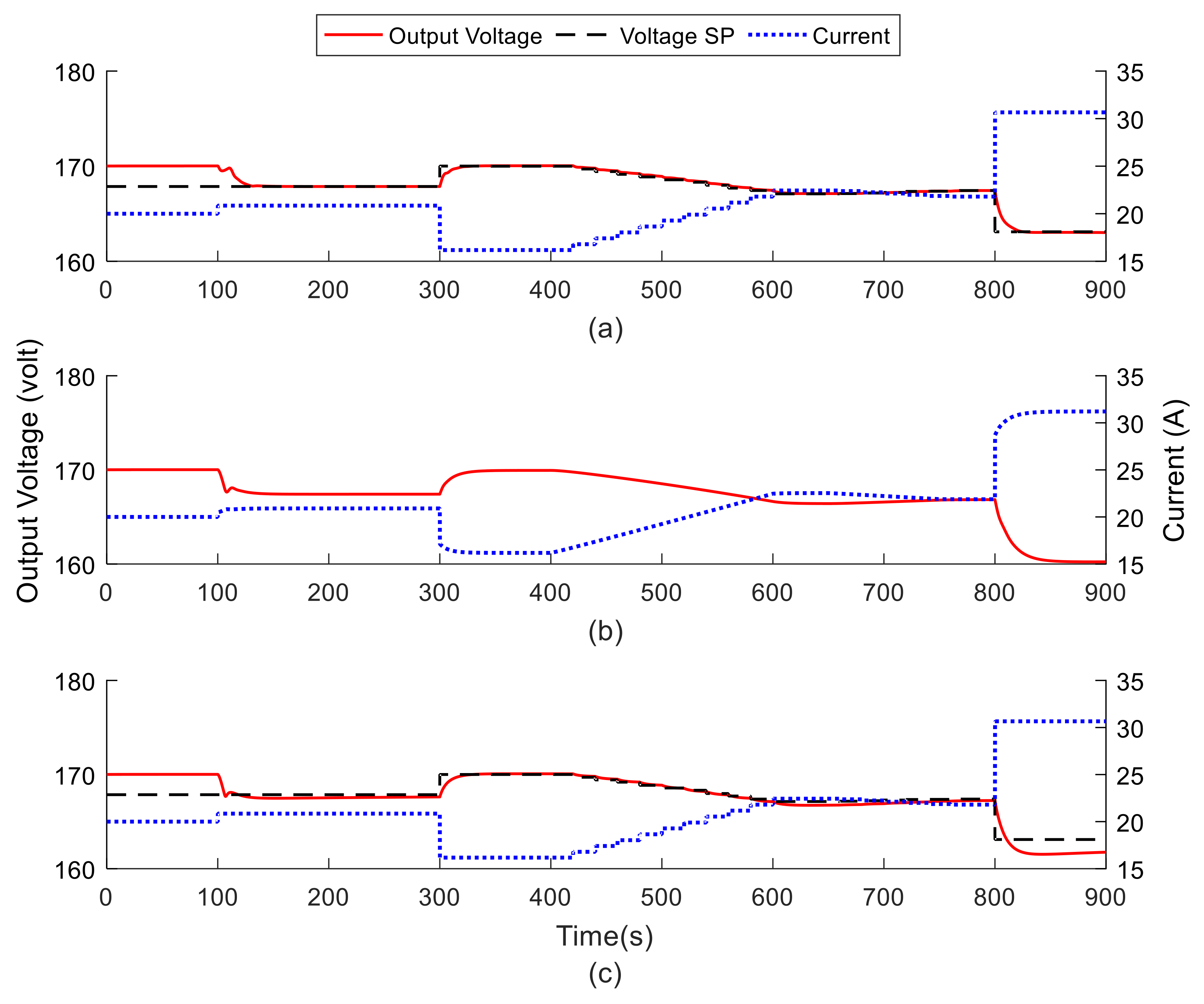
The power tracking performance of the system without SP scheduler is almost as good as that of the system with the proposed control strategy. The reason is that the PID-only control architecture directly controls the output power through changing the current. The architecture in fact avoids the nonlinearity associated with the SOFC. Nevertheless, when checking the waste power of the SOFCs in Figure 9, the system without SP scheduler turns out to be with the highest waste power. The SP + PID system does not have as good economic performance as the one with proposed control strategy since it actually does not track the set points of output voltage and current so well, despite the fact that both of them receives optimal SPs from the SP scheduler. This explanation can be verified by the curves of output voltage and current in Figure 10. 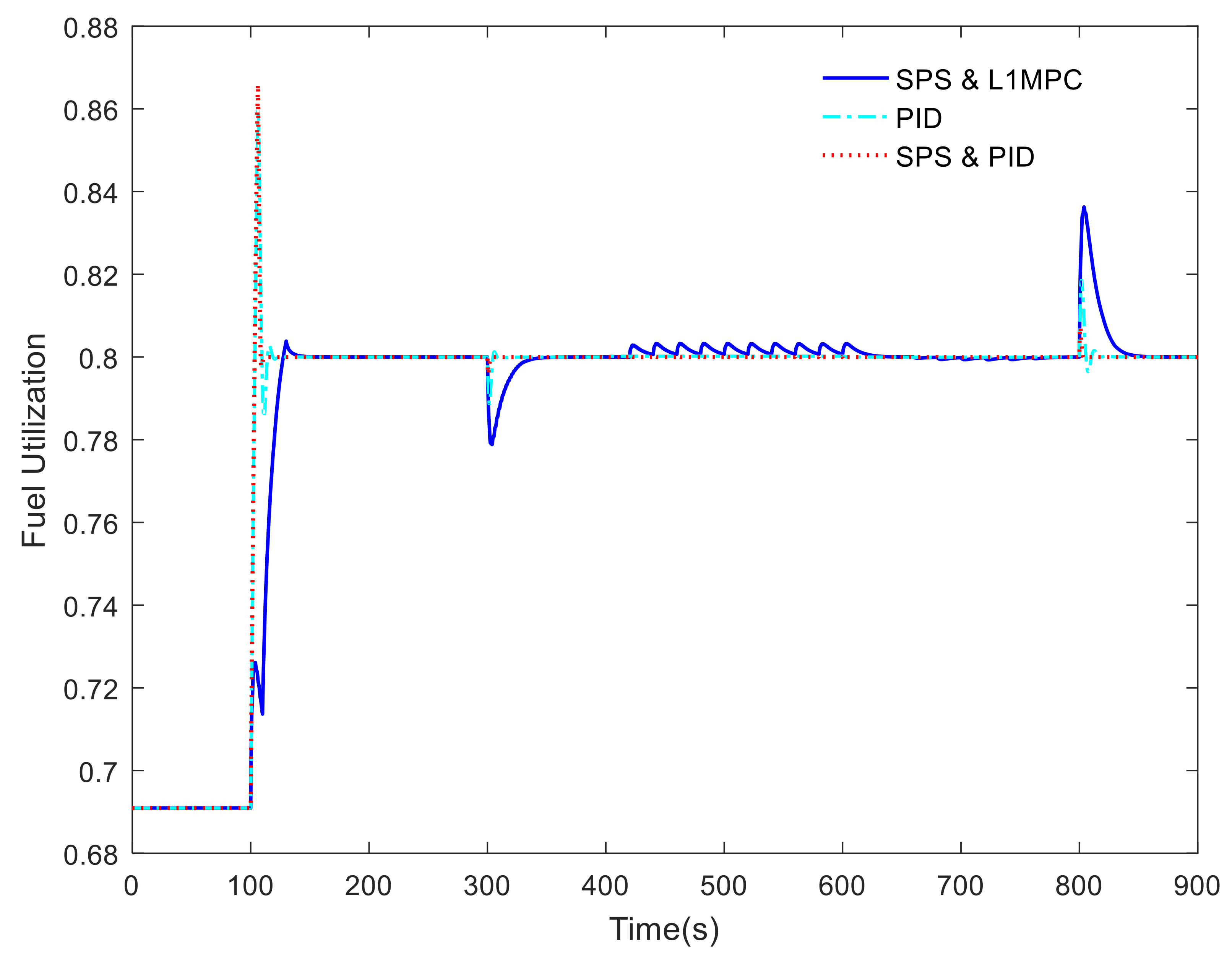Figure 11 presents the fuel utilization curve. Both of the three control methods can handle the fuel utilization in the safe range. The proposed control strategy has a more flexibility action of the manipulated inputs in order to have better tracking performance. As a consequence, the deviation of FU to the expected value is larger than the other two systems in some transient states. Nevertheless, the safe range of FU is always guaranteed because of the protective mechanism employed in this work. 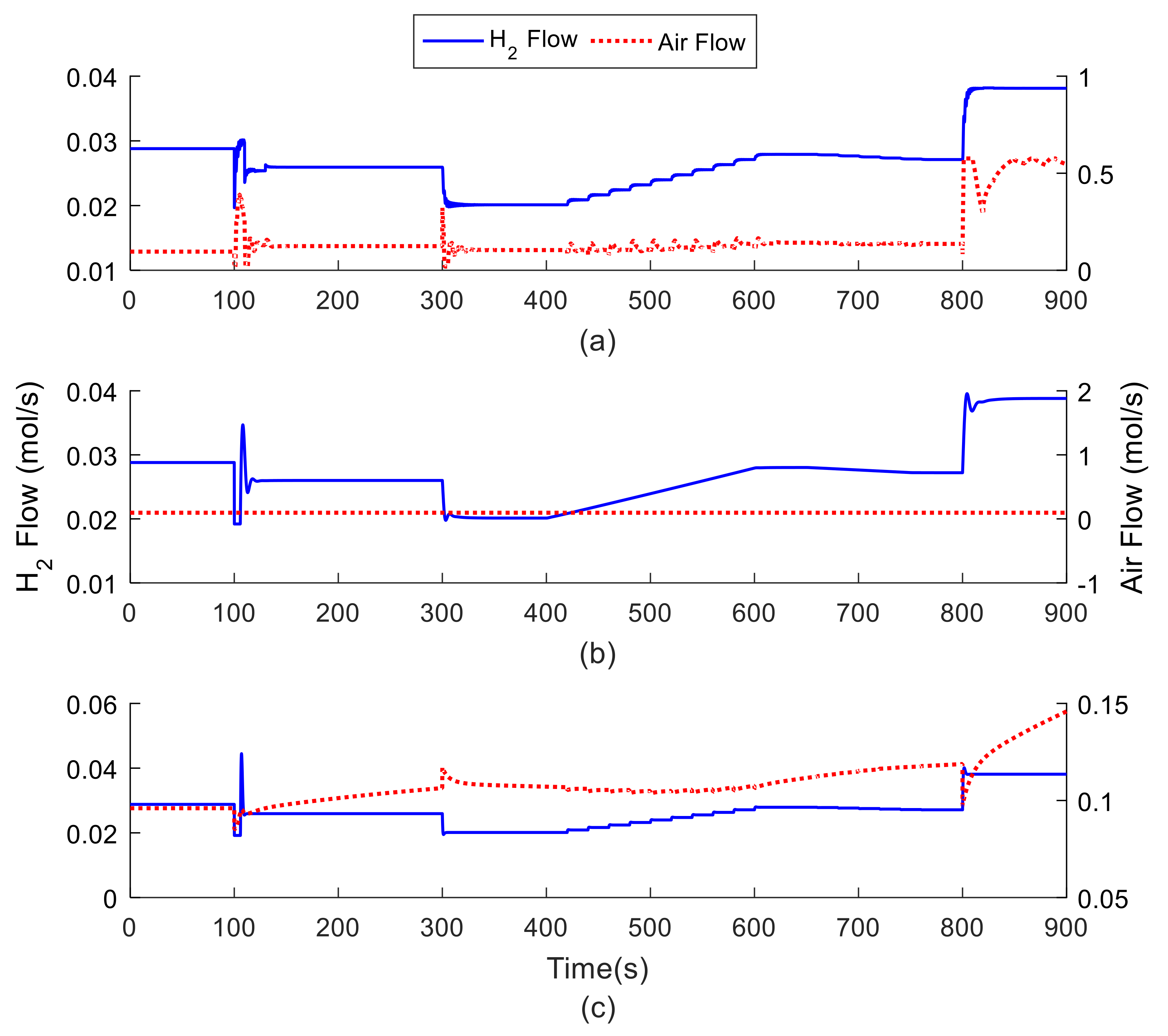Figure 12 shows the manipulated inputs of the SOFCs. The SOFCs are with different steady-state temperature under different load. Since the thermo-dynamic process is so slow that by the end of the simulation, the temperature has actually not reached a new steady state. This causes a continuous regulating of the inlet air flow in order to compensate for the voltage perturbation brought by the temperature change.

Based on the simulation results, the features of the proposed control strategy are concluded in

Table 3. The conducted simulation and expected performance.

Simulation No.	Tracking Controller	With SP Scheduler?	Constraint Guaranteed?	SP Tracking Performance (Rank)	Economic Performance
1	L1-MPC	Yes	Yes	Best	Best
2	PID	No	No	Worst	Worst
3	PID	Yes	No	Medium	Medium

along with that of the two comparative simulation. By comparing the Simulation 1 (the proposed control strategy) and Simulation 3 (SP Scheduler + PID), the advantage of the proposed L1-MPC in tracking performance and constraint satisfaction is highlighted. It is worth pointing out that the L1 adaptive controller is the key technique that contributes to the tracking performance. It is well-known that the performance of MPC depends on the their tuned parameters. The most contributing parameters for a linear-model based MPC is the weight matrix Q and R, in (56). Trade-offs can be made between tracking performance and robustness by tuning Q and R. When the plant are with nonlinearities, the MPC have to be tuned in a robust way in order to guarantee the stability of the system when the operation point deviates from the nominal one. In this case, the control action is usually conservative, thus the performance is sacrificed. In our work, we add a L1 adaptive control term in the control signal (52), the nonlinearity of the system dynamic is compensated in a fast way. In this case, the MPC parameters can be tuned in more aggressive way, aka, being able to achieve better tracking performance.

Similarly, The PID controller in Simulation 3 has to be tuned sufficiently conservative to guarantee with the existence of system nonlinearity, although it has the potential to have a better performance when working in a small range of working conditions. We highly recognize that there exist plenty of advanced PID that can deal with the system nonlinearities. However, it is out of the scope of this paper. We will not make further discussion here although it can be a very attractive work in the future.

The comparison between Simulation 3 and Simulation 2 (Only PID) further shows the effect of set point scheduler to achieve a better economic performance of the SOFCs. Indeed, in Simulation 3, we have implemented an entirely difficult control structure. However, this is the plainest way to make power command tracking with constant fuel utilization maintained.

6. Conclusions

This paper proposes a procedure to design a hierarchical control strategy for optimal power tracking operation of grid-connected SOFCs. The control strategy consists of a set point scheduler in the upper level and a SOFC controller working together with VSI devices in the lower level. The setpoints scheduler finds the optimal values of output voltage and current minimizing the internal waste power, based on a comprehensive steady-state model of the SOFC. The acquired optimal values are transmitted to the lower-level SOFC controller and VSI device as their set points. To overcome the insufficiency of MPC in dealing with the nonlinearities and uncertainties in the system dynamics, a combined L1-MPC control algorithm is put forward in the SOFC controller design. Additional protection logic is included in the control strategy to prevent SOFC from fuel starvation under unit load demand variation within the SOFC controller’s the sampling interval. The simulation result shows the superiority of the proposed method.

A future direction of effort might be improving the economy in the system’s transient states. The set point scheduler optimizes the system economy merely in steady states. However, when the micro-grid has frequent demand for peaking regulation, the unit load demand would change continually. In this case, the SOFC system rarely operates in steady states. Actually, this situation is very likely to happen in those micro-grids operating in islanding mode. As a consequence, the economy in transient process becomes crucial to the general economy of the SOFCs. It will be of great interest in the future to apply those approaches to take care of the plant’s economy in the transient process.