Article

Forecasting Energy-Related CO2 Emissions Employing a Novel SSA-LSSVM Model: Considering Structural Factors in China

1
School of Economics and Management, North China Electric Power University, Beijing 102206, China
2
Beijing Key Laboratory of New Energy and Low-Carbon Development, North China Electric Power University, Changping, Beijing 102206, China
*
Author to whom correspondence should be addressed.
Energies 2018, 11(4), 781; https://doi.org/10.3390/en11040781
Submission received: 14 February 2018 / Revised: 18 March 2018 / Accepted: 23 March 2018 / Published: 28 March 2018

Abstract

:
Carbon dioxide (CO2) emissions forecasting is becoming more important due to increasing climatic problems, which contributes to developing scientific climate policies and making reasonable energy plans. Considering that the influential factors of CO2 emissions are multiplex and the relationships between factors and CO2 emissions are complex and non-linear, a novel CO2 forecasting model called SSA-LSSVM, which utilizes the Salp Swarm Algorithm (SSA) to optimize the two parameters of the least squares support sector machine (LSSVM) model, is proposed in this paper. The influential factors of CO2 emissions, including the gross domestic product (GDP), population, energy consumption, economic structure, energy structure, urbanization rate, and energy intensity, are regarded as the input variables of the SSA-LSSVM model. The proposed model is verified to show a better forecasting performance compared with the selected models, including the single LSSVM model, the LSSVM model optimized by the particle swarm optimization algorithm (PSO-LSSVM), and the back propagation (BP) neural network model, on CO2 emissions in China from 2014 to 2016. The comparative analysis indicates the SSA-LSSVM model is greatly superior and has the potential to improve the accuracy and reliability of CO2 emissions forecasting. CO2 emissions in China from 2017 to 2020 are forecast combined with the 13th Five-Year Plan for social, economic and energy development. The comparison of CO2 emissions of China in 2020 shows that structural factors significantly affect CO2 emission forecasting results. The average annual growth of CO2 emissions slows down significantly due to a series of policies and actions taken by the Chinese government, which means China can keep the promise that greenhouse gas emissions will start to drop after 2030.

1. Introduction

The issue of climate change has become the focus of attention of all countries in the world, and CO2 emissions are considered as the main factor of global warming [1]. The recently agreed agreement, known as the “Paris Accord,” specifically identifies the target of a temperature increase of less than 2 degrees Celsius as compared to the pre-industrial era [2]. China accounts for 23% of global energy consumption and 27% of global energy consumption growth [3]. China accounted for 28.77% of the global total CO2 emissions in 2015, reaching 36.2 billion tons according to the global carbon project website statistics, more than the sum of the United States and the European Union, which means China is the world’s largest greenhouse gas emitter and energy consumer [4]. China promises that greenhouse gas emissions will start to drop after 2030 and has recently taken a series of measures to achieve its emission reduction targets [5,6]. Coal’s share of China’s energy mix dropped from 64% in 2015 to 62% in 2016, and China’s coal output fell 7.9%, which is the largest annual drop since tracking the data from 1981. In 2016, China’s CO2 emissions decreased for the second consecutive year, a decrease of 0.7% [3]. CO2 emissions growth presents a new trend affected by various policy implementations in China, so it is critical to forecast CO2 emissions from the perspective of energy consumption considering the role of different policies. CO2 emissions forecasting helps to predict the global temperature and contribute to verifying the possibility of achieving the 2 °C goal under current policy efforts [7].
Research on the influential factors of CO2 emissions has been widely implemented recently. Economy and energy consumption are regarded as the main factors of CO2 emissions in some research. Behnaz Saboori [8] studied the relationships between economic growth, energy consumption and CO2 emissions using data of the five Association of Southeast Asian Nations countries by Auto-regressive Distributed Lag (ARDL) methodology and Vector Error Correction Model (VECM); the results showed that the relationship between CO2 and economic growth is non-linear for the cases of Thailand and Singapore, and energy consumption and CO2 emissions have bi-directional causality in the five countries. Mohamed El Hedi Arouri [9] found that energy consumption is positively correlated with CO2 emissions, and GDP and CO2 emissions show a quadratic curve relationship in 12 Middle East and North African countries. Some recent studies on this topic were implemented in different countries, i.e., France [10], the United States [11], China [12], India [13], Iran [14], and Turkey [15]. However, a lack of consensus was found among these studies, indicating the relationships of economic growth, energy consumption and CO2 emissions are complicated. People are producers and consumers of fossil energy. Changes in the population should, as a matter of course, affect CO2 emissions. Tom Knapp [16] found the relationship between global population growth and CO2 emissions lacks a long-term equilibrium, but indicated a short-term dynamic relationship. Qin Zhu [17] expanded the STRIPAT model to examine the relationship between population and CO2 emissions in China from 1978 to 2008 and revealed CO2 emissions in China will continue with an upward trend for the next two decades in response to population growth. Some other researches also showed that the population is one of the key factors affecting CO2 emissions [18,19,20]. Urbanization means more industrial production and energy consumption, so urbanization has a certain impact on CO2 emissions. Cole [21], Liddle [22], and Fan et al. [23] studied the relationship between urbanization and CO2 emissions by using panel data. However, their results lack consensus. Inmaculada Martínez-Zarzoso [24] researched the relationship between urbanization and CO2 emissions in developing countries from 1975 to 2003 and showed an inverted-U shaped. CO2 emissions continue to increase with urbanization, and when it reaches a certain level, its impact on CO2 emissions becomes negative. Therefore, the relationship between urbanization and CO2 emissions could be non-linear. The economic structure is generally expressed as the proportion of secondary industry, which is also called the industrial structure. Zhang X [25] found a long-term stable equilibrium relationship between industrial structure and CO2 emissions in Shandong province by Granger causality test, and industrial structure affected CO2 emissions, i.e., changes in industrial structure curbed the emissions in 1994–1999 and 2006–2009, which means industrial structure has different contributions to CO2 emissions in different stages. PhilipKofi Adom [26] studied the short-term causal relationships and long-term equilibrium relationships among CO2 emissions, economic growth, technical efficiency, and industrial structure for three African countries. Changing the industrial structures encourages the expansion of low energy intensive or high-technology efficient industries that are emphasized in the conclusion. With the development of clean energy, the proportion of coal consumption continues to decrease, which is the most important source of CO2 emissions. The impact of energy structure on CO2 emissions will be increasingly significant. Zheng Wang [27] constructed a hybrid energy model that aims to minimize costs, and the simulation result shows that China will achieve peak CO2 emissions in 2025 due to energy structural change. Shibao Lu [28] established the low-carbon city development model and found that under the same rate of economic growth, the lower the secondary industry proportion, the smaller the carbon intensity. In addition to the factors mentioned above, the impact of energy intensity on CO2 emissions has drawn more and more scholars’ attention. Muhammad Shahbaz [29] found that energy intensity increases CO2 emissions; the feedback hypothesis between energy intensity and CO2 emissions is verified by VECM causality analysis. Lin Boqiang [30] explored the factors of CO2 emissions of China’s heavy industry by the Logarithmic Mean Divisia Index (LMDI) method based on the extended Kaya identity, and the result showed that energy intensity is one of the main factors, and a decline in energy intensity leads to a reduction in CO2 emissions. Minda Ma’s research indicated that the building energy efficiency declining contributed to significantly positive CO2 emissions reduction in China’s public buildings from 2001 to 2015 [31]. Rina Wu [32] drew the same conclusion for industrial sector CO2 emissions in Inner Mongolia.
Most research about CO2 emissions reduction focuses on the traditional influential factors, but carbon capture technology has become an important factor that contributes to CO2 emissions reduction, and many scientists believe carbon capture technologies will determine the realization of the target 2 °C global temperature increase directly. Carbon dioxide capture and storage (CCS) technologies can reduce CO2 emissions from coal-fired power generation by up to 90% [33] and can effectively reduce the variability and intermittent behavior of renewable energy generation [34]. Cryogenic carbon capture (CCC) is one of the main CCS technologies, and it separates solid CO2 from the remaining cooled gas and melts, which are generated from the power generation units. Safdarnejad S M [35] constructed a hybrid system by combining cryogenic carbon capture with a baseline fossil-fueled power generation unit, and it is optimized by utilizing the combination of coal, gas, and wind power sources with priority given to wind power to meet the electricity demand. It was found that the energy storage of cryogenic carbon capture contributes to a saving of the cycling costs. He also constructed a hybrid system including load-following coal and gas-fired power units, a CCC process, and wind generation. The objective of this system is to meet the electricity demand and maximize the profit at the same time. The results indicated that this hybrid system can result in an average profit of $35 k/h [36]. Kang C A [37] optimized a flexible coal-natural gas power station with CCS to overcome the drawbacks of CCS. The differences in scenario results in West Texas, the United Kingdom, and India illustrate the great impact of economic forecasts on optimal facility design. Gopan A [38] proposed a novel Staged, Pressurized Oxy-Combustion (SPOC) process and constructed a conceptual power plant with the SPOC method. The results show that the efficiency improved over 6 percentage points compared with first generation atmospheric oxy-combustion technology, which means SPOC makes up for the loss of efficiency due to carbon capture technology. Membranes [39,40] are another way to capture carbon, and Rezakazemi M [41] summarized the current status and future directions of mixed matrix membranes (MMMs), which will promote the development of carbon capture technologies.
The forecasting models of CO2 emissions have been developed in recent years. Some scholars forecast CO2 emissions through traditional econometric methods. J. Wesley Burnett [42] estimated the relationships between CO2 emissions and factors by using a long panel data set in different U.S. states. Besma Talbi [43] used the Vector Auto-Regressive (VAR) model to analyze CO2 emissions reduction in the road transport sector in Tunisia. Ahmed [44] investigated the relationship between the main influential factors and CO2 emissions in Pakistan by co-integration combined with the ARDL bounds testing method based on the Environmental Kuznets Curve (EKC) hypothesis. Relationships between all factors and CO2 emissions are regarded as linear in econometric methods which is inconsistent with the actual situation. Kumar [45] constructed different energy scenarios by the Long-range Energy Alternatives Planning System (LEAP) method and estimated CO2 emissions with the least cost method; the finding showed that the CO2 emissions could decrease 74% by 2050 under the accelerated renewable energy technology scenario. Liu [46] and Chang [47] also applied the LEAP model to estimate CO2 emissions of the Jiangxi transportation industry and Shanghai. The deficiency of the LEAP model is that the judgment of experts is subjective. Li [48] calculated the CO2 emissions reduction potential under different scenarios for 2016 and 2020 in Beijing by a BP neural network optimized by the improved particle swarm optimization algorithm, which may lead to a low precision model, premature or over-fitting problem. Liang [49] constructed an input-output model for China’s multi-region energy consumption and CO2 emissions, and conducted a scenario analysis for 2010 and 2020. The Gray model (GM) has been widely used due to its own advantages. Lin [50] and Pao [51] utilized the gray model to predict CO2 emissions of Taiwan and Brazil. Some improved gray models are proposed to estimate CO2 emissions [52,53], but their ability to forecast long-term is poor, and the more samples selected, the greater the number of errors [54]. The relationships between CO2 emissions and influential factors are non-linear and complicated, which is not reflected in the previous studies. Therefore, intelligent forecasting techniques can be employed in CO2 emissions, which have a highly accurate learning and forecasting ability. This paper tries to predict CO2 emissions by using the LSSVM model, which is a widely used and related supervised learning method.
The forecasting accuracy of the LSSVM model depends on the values of two parameters, namely, the regularization parameter “ c ” and the bandwidth of the radial basis function (RBF) kernel “ σ ”. It is common to utilize optimization methods to obtain the best values of the two parameters. Dongxiao Niu [55] used a modified particle swarm optimization algorithm and LSSVM based on the denoising method of empirical mode decomposition and a gray relational analysis model to predict the short-term electric load. Weishang Guo [56] proposed a novel hybrid combining the Beveridge-Nelson decomposition method, fruit fly optimization algorithm, and LSSVM model for electricity price forecasting. Qunli Wu [57] applied the LSSVM model optimized by a cloud-based evolutionary algorithm for accurate wind power generation prediction. Wei Sun [58] constructed a novel hybrid model based on principal component analysis and LSSVM optimized by cuckoo search to forecast the daily PM2.5 concentration, which presents a strong potential. The LSSVM model is widely applied in different fields for forecasting issues except CO2 emissions. There are also many optimization methods, such as fruit fly optimization (FOA) [59], genetic algorithm (GA) [60], and artificial bee colony algorithm (ABC) [61]. However, most of the optimization algorithms have some shortcomings such as falling into a local optimal solution and slow iteration. Therefore, this paper employed SSA to optimize the two parameters of LSSVM, which was first proposed by Seyedali Mirjalilli in 2017. It is theoretically and potentially able to solve single-objective optimization problems with unknown search spaces, and the adaptive mechanism of SSA allows this algorithm to avoid local solutions and eventually obtain an accurate estimation of the best solution during optimization [62]. Considering the superiority of SSA, the SSA-LSSVM model is constructed to improve the forecasting performance and accuracy of CO2 emissions.
Taking China’s social and economic development, industry structure and energy structure adjustment, energy conservation and environmental protection efforts into account, the main factors of CO2 emissions are GDP, population, energy consumption, economic structure, energy structure, urbanization rate, and energy intensity in this paper, which are also regarded as the input variables for the constructed SSA-LSSVM model. Carbon capture technologies are difficult to quantify in the model; therefore, the impact on CO2 emissions of carbon capture technologies is not considered in this paper. The development level of each factor is calculated according to the development plans, and the CO2 emissions from 2017 to 2020 in China are forecast by the SSA-LSSVM model.
The main contributions of this article are as follows:
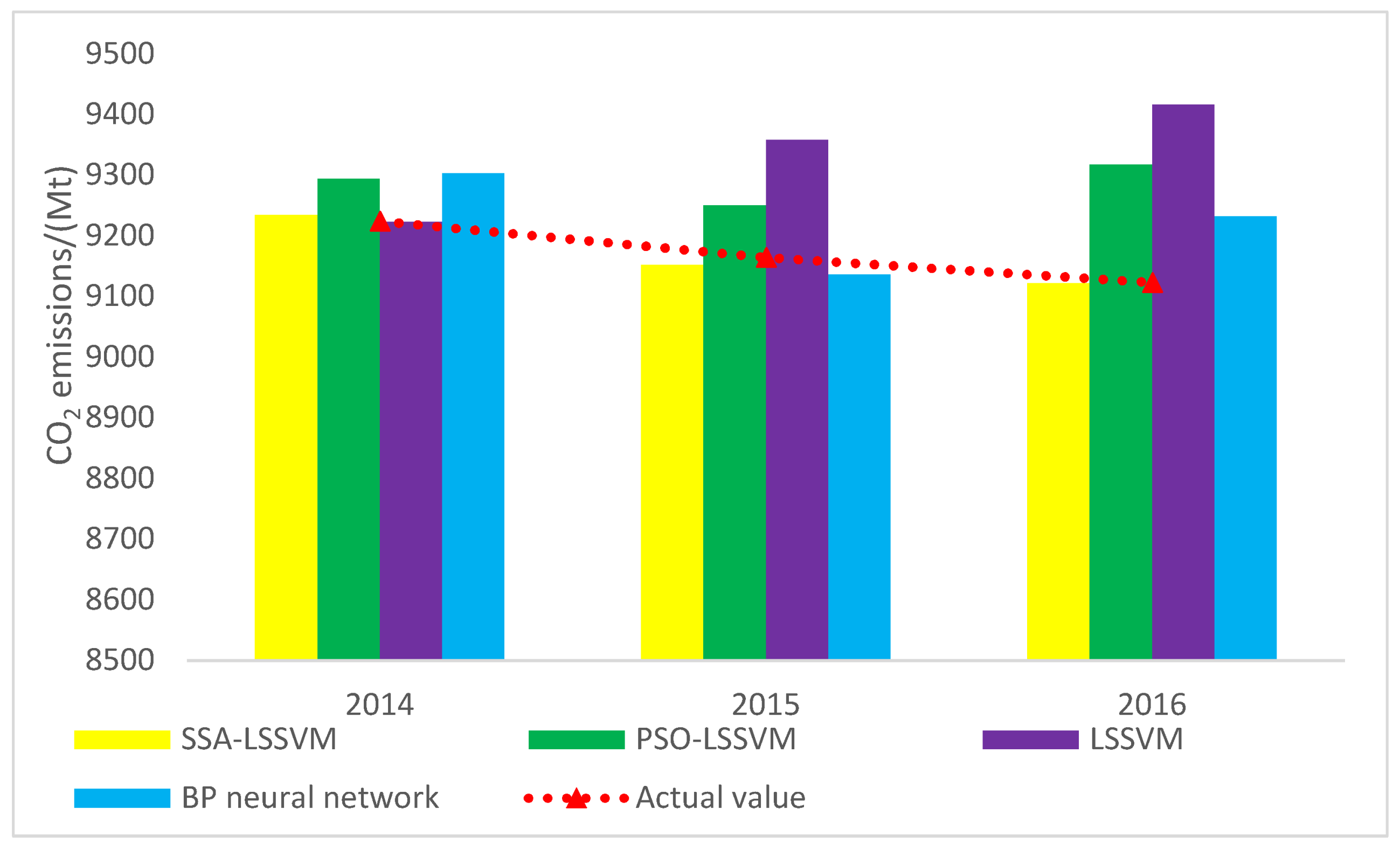
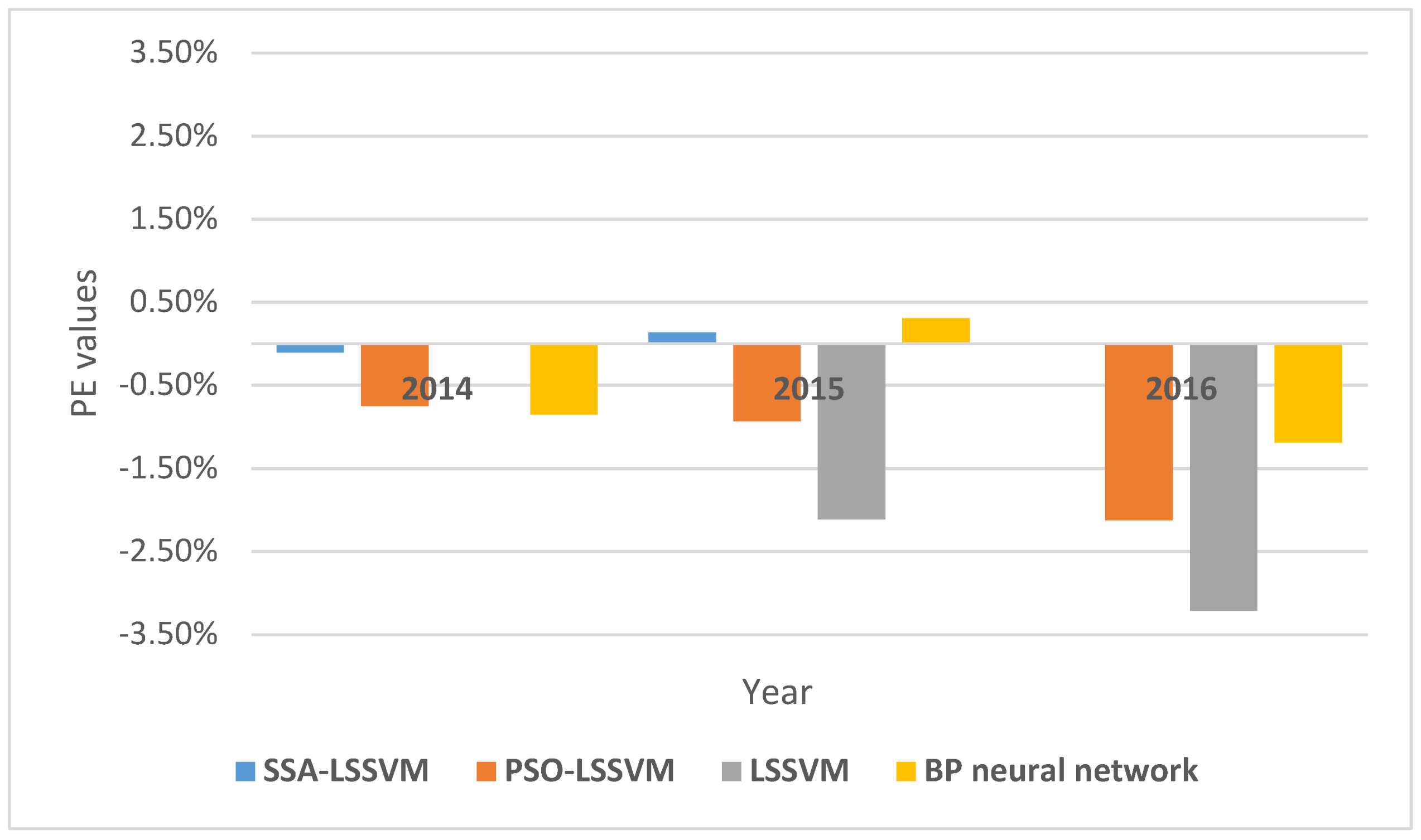
  • A novel LSSVM model optimized by SSA (SSA-LSSVM) for CO2 emissions forecasting is proposed, which has superiority in the forecasting accuracy of CO2 emissions compared with the single LSSVM model, PSO-LSSVM model, and BP neural network model. The SSA-LSSVM model is verified to be suitable for CO2 emissions forecasting.
  • Economic structure, energy structure, urbanization rate and energy intensity are taken into consideration in the proposed model as the driving factors of CO2 emissions, which reflect the orientation of China’s recent policies that aim to keep the promise of CO2 emissions reduction by 2030, and all structural factors affect the forecasting value significantly.
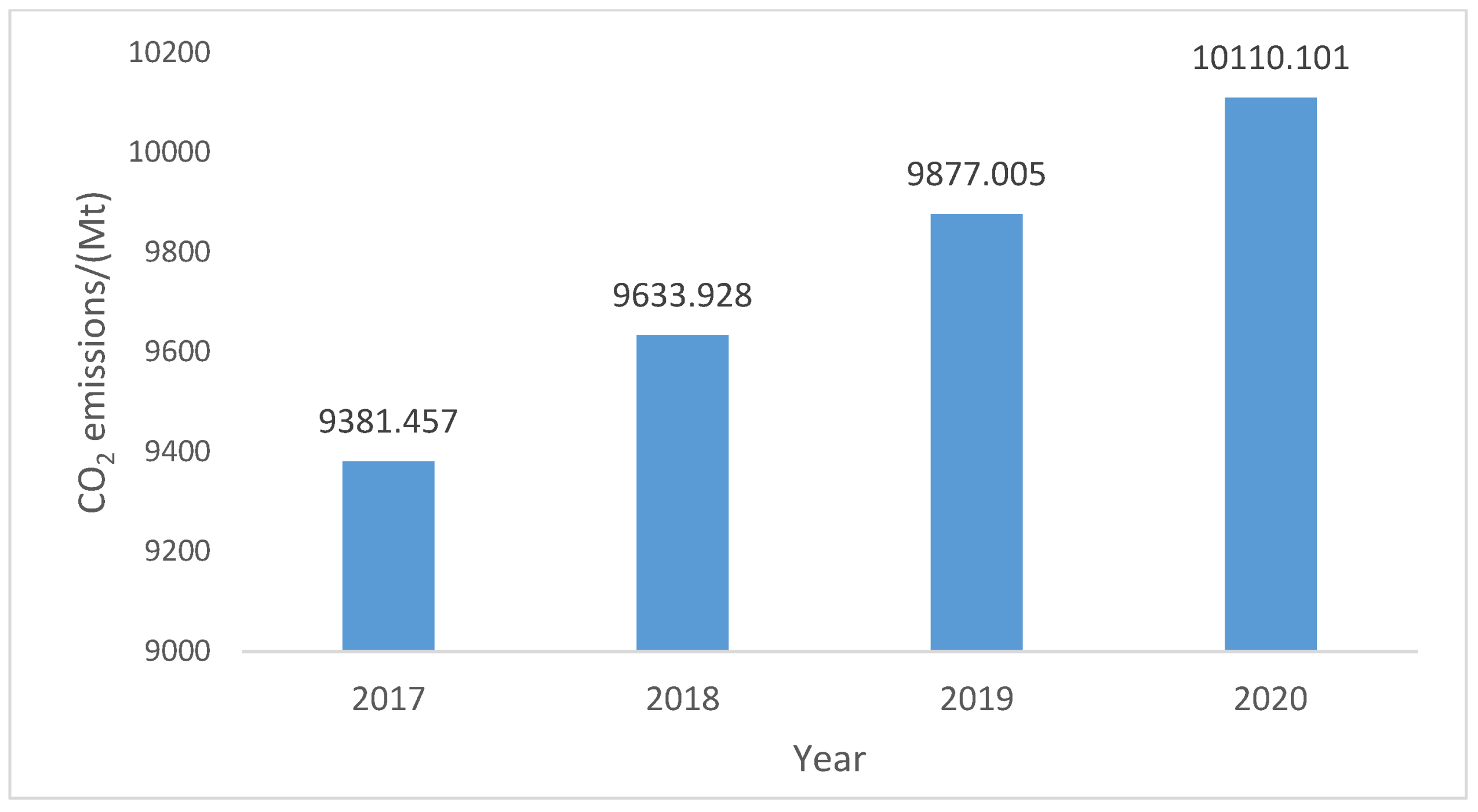
  • According to the social, economic and energy requirements of the 13th Five-Year Development Plan, the SSA-LSSVM model is used to forecast CO2 emissions in China from 2017 to 2020, and the future growth trend and the reasons for the change are analyzed in this paper.
The main structure of this paper is as follows. Section 2 presents the theory of the SSA and LSSVM model, and the novel SSA-LSSVM model is proposed for CO2 emissions forecasting, which is a combination of the SSA method and LSSVM model. Section 3 presents an empirical analysis of CO2 emissions in China based on the SSA-LSSVM model, and the superiority of the proposed model is verified compared with other methods. In Section 4, CO2 emissions in China from 2017 to 2020 are forecast, and the development trend is analyzed. Finally, the conclusions are drawn in Section 5.

2. The Methodology of the SSA-LSSVM Forecasting Model

2.1. The Basic Methodology of the LSSVM Model

LSSVM is a form of support vector machines (SVM) under the quadratic loss function. It replaces the quadratic programming solver optimization problem by solving the linear equation, which possesses advantages of simplifying the model and a rapid solving ability without losing accuracy [63,64,65]. The basic theory of LSSVM is described below.
For a training sample set: S = ( x i , y i ) i = 1 l , x X R n is the input vector and y R is the output value corresponding to the sample; the following decision function can be constructed as a learning machine.
f ( x ) = ω · φ ( x ) + b
where φ is the input vector; φ ( x ) is a linearly separable nonlinear high-dimensional map; ω is the weight vector; b is the offset value.
The structural risk function is as follows:
R = 1 2 ω 2 + 1 2 C · R e m p
where ω 2 is the complexity of the control model; C is the normalization parameter; R e m p is the empirical risk.
In the LSSVM model modeling process, R e m p can be expressed as the following quadratic expression, and the optimization problem can be expressed as:
Minimize   χ = 1 2 ω T ω + 1 2 C · i = 1 l ξ i 2
Subject   to   y i = ω T · φ ( x i ) + b + ξ i
where ξ is the error slack variable, i = 1 , 2 , , l .
Using the Lagrange multiplier and the dual transformation method to transform the above programming problem, the following Lagrange function can be obtained:
L ( ω , b , ξ , α ) = 1 2 ω T ω + 1 2 C · i = 1 l ξ i 2 i = 1 l α i [ ω T · φ ( x i ) + b + ξ i y i ]
According to the Karush-Kuhn-Tucker (KKT) condition, the following equation is obtained:
{ L ω = 0 L b = 0 L ξ = 0 L α = 0
The above equation is equivalent to the following formula:
{ ω i = 1 l α i · φ ( x i ) = 0 i = 1 l α i = 0 α i = C · ξ i ω T · φ ( x i ) + b + ξ i y i = 0
Construct the following kernel function that satisfies the Mercer’s theorem:
K ( x , z ) = φ T ( x ) · φ ( z )
Equation (7) can be expressed as:
[ 0 I v T I v Ω + C 1 I ] [ b α ] = [ 0 y ]
where I V = [ 1 , 1 , , 1 ] T contains l elements; Ω i j = K ( x i , x j ) , i , j = 1 , 2 , , l .
The available kernel functions in the LSSVM model include the Sigmoid kernel function, Polynomial kernel function and Radial Basis Function (RBF) kernel function. The RBF kernel function has been applied in many practical problems due to the fewer parameters that need to be preset and the adaptation to practical problems. Therefore, this paper uses the RBF function as the kernel function of the LSSVM model, namely:
K ( x , z ) = exp ( x z 2 σ 2 )
After selecting the appropriate kernel function to solve the nonlinear regression problem, we can solve Equation (8), and then we can obtain the decision function:
f ( x ) = i = 1 l α i K ( x i , x ) + b
In the above formula, two parameters need to be confirmed, including regularization parameter c and kernel function parameter σ . This paper utilizes the SSA method to search the optimal values of c and σ of the LSSVM model and forecast CO2 emissions accurately. The theory of SSA algorithm and the optimization details are expounded in Section 2.2 and Section 2.3.

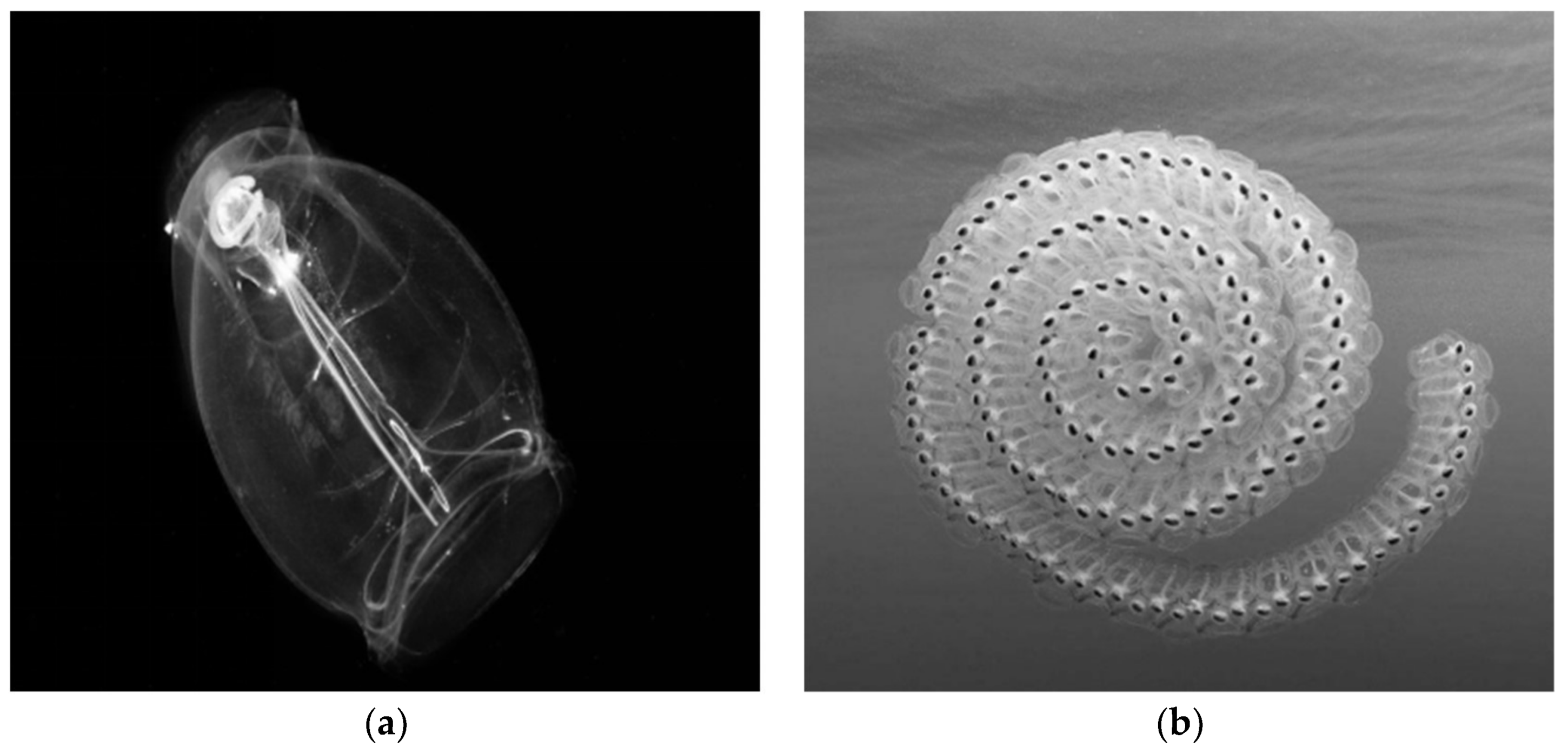
2.2. The Basic Theory of SSA

Salps have a transparent and barrel-shaped body and belong to the family Salpidae. They move forward by pumping water through their body as a driving force similar to jelly fish [66]. Research about salps is rare due to the fact that the living environment is very difficult to access, which is usually in the deep sea. Salps exhibit swarming behavior; they form a swarm called a salp chain, which is believed to achieve better movement through rapid coordination of changes and forage [67]. Individual salps and this chain are illustrated in Figure 1. Seyedali Mirjalili proposed a novel heuristic optimization method, namely SSA, based on the salp chain behaviour. In the SSA method, the population is divided into a leader, which is at the front of the chain, and followers; the leader guides the salp chain and the followers follow one by one. It is assumed that there is a food source set as the salps chain target in the search space called F. For details of SSA refer to Seyedali Mirjalili’s research paper [62].
In accordance with the behaviour of a salp chain, several steps are made to explain the SSA method, which are illustrated as follows:
Step 1
Parameters setting.
The main parameters of SSA include the number of search agents SearchAgents_no; maximum number of iterations Max_iteration; the number of variables (dimension of the problem) dim; the upper bound ub = [ub1, ub2, ub3, …, ubn−1, ubn] and the lower bound lb = [lb1, lb2, lb3, … lbn−1, lbn], i.e., the variables.
Step 2
Population initialization.
Initialize the salp population with random positions in SSA, and the position matrix is as below:
S = [ s 11 s 12 s 1 d s 21 s 22 s 2 d s n 1 s n 2 s n d ]
where S represents the position matrix of the salp chain, sij represents the value of the j-th variable of the i-th salp, i = 1, 2, …, n, j = 1, 2, …, d, sij is calculated by the following Equation (12) with a stochastic distribution.
S ( i , j ) = r a n d ( i , j ) × ( u b ( i ) l b ( i ) ) + l b ( i )
where S(i,j) represents the value of the i-th row, j-th column in the matrix. rand(i,j) is a stochastic matrix with all elements distributed in [0, 1] interval. ub(i) and lb(i) represent the upper bound and lower bound of the i-th salp respectively.
Step 3
Fitness function construction.
The fitness function is to calculate the fitness value of each salp, which is determined during the process of optimization, and the all values are stored in the matrix OS as follows:
O S = [ O S 1 O S 2 O S n ] = { f [ ( s 11 s 12 s 1 d ) ] f [ ( s 21 s 22 s 2 d ) ] f [ ( s n 1 s n 2 s n d ) ] }
In the matrix OS, the position of the salp with best fitness value is assigned to be the variable F as the source food, which is chased by the salp chain. Therefore, a moving food source makes it possible to obtain the global optimum.
Setp 4
Iteration process.
In order to perform global searching and avoid local optimum, all salps renovate their position by special methods in the SSA method.
For the leader’s position updating with respect to the food source, the following Equation (14) is implied:
x j 1 = { F j + c 1 ( ( u b j l b j ) c 2 + l b j ) F j c 1 ( ( u b j l b j ) c 2 + l b j ) c 3 0 c 3 < 0
where in the j-th dimension, x j 1 indicates the position of the leader (first salp), Fj is the food source’s position, ubj and lbj indicate the upper bound and lower bound respectively, c1, c2, c3 are all random numbers. c2 and c3 are generated in the interval of [0, 1], which determine iteration direction of the next position in the j-th dimension and step size. c1 is a critical parameter in SSA due to balancing exploitation and exploration; it is defined as below:
c 1 = 2 e ( 4 l L ) 2
where L is the maximum number of iterations, and l is the current iteration.
Newton’s law of motion is utilized to update the position of the followers; the equation is shown as follows:
x j i = 1 2 a t 2 + v 0 t
where i 2 , x j i is the i-th follower salp’s position in the j-th dimension, t is time, a = v f i n a l v 0 and where v = x x 0 t . v0 indicates the initial speed.
Considering the discrepancy is equal to 1 in the iteration process and v0 = 0, Equation (16) can be simplified as follows:
x j i = 1 2 ( x j i + x j i 1 )
All steps are executed in the iteration process except initialization until reaching the ending standard of the SSA method iteration.

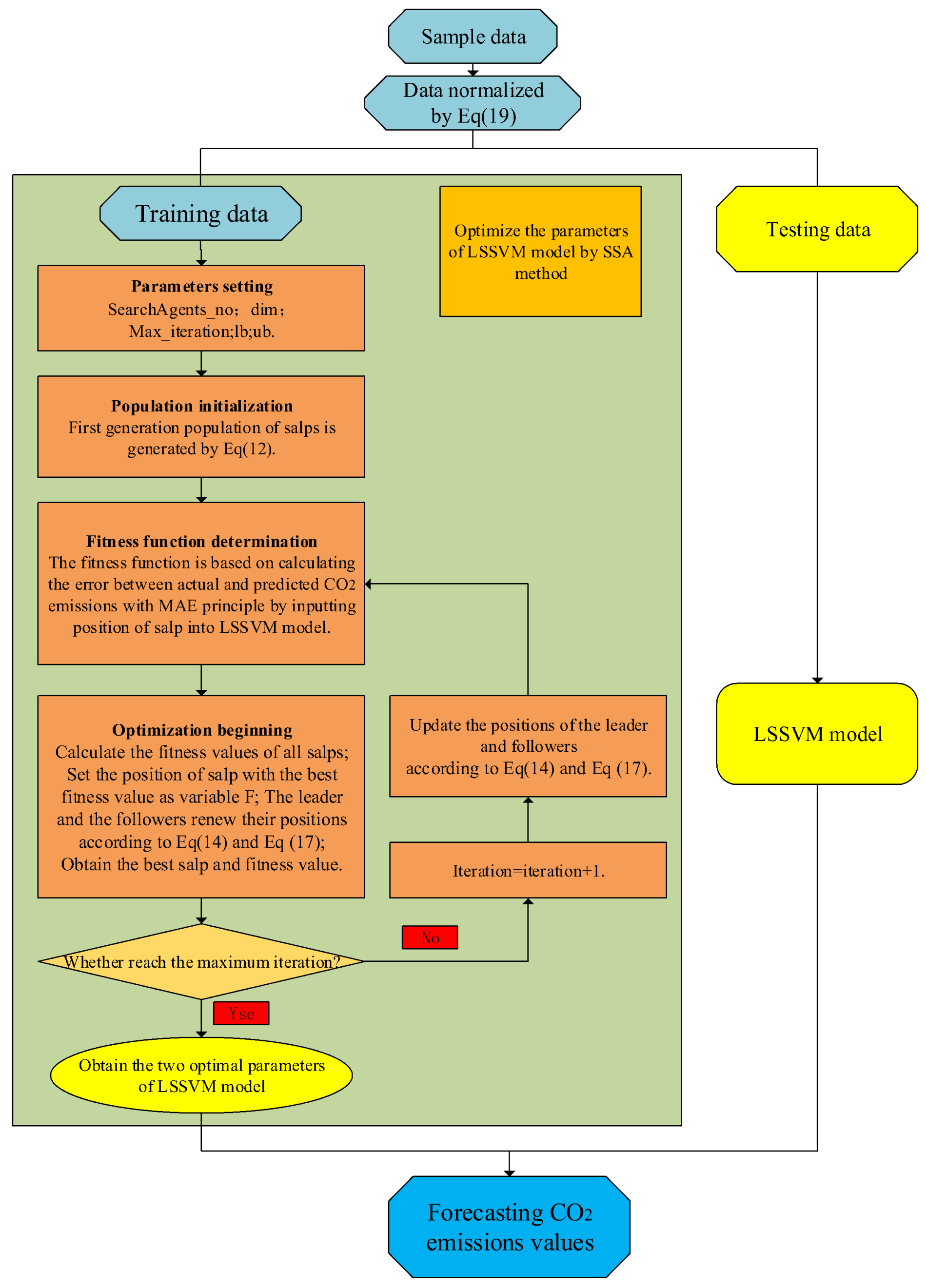
2.3. Primary Principle of the SSA-LSSVM Model for CO2 Emissions Forecasting

In order to improve the forecasting performance, the SSA method is utilized to determine the two parameters of the LSSVM model; therefore, the CO2 emissions forecasting model based on the SSA-LSSVM method is proposed. The main process of the SSA-LSSVM model is elaborated on below:
Step 1
Set parameters.
The main parameters of SSA include: the number of search agents Search Agents_no; maximum number of iterations Max_iteration; the number of variables (dimension of the problem) dim; the upper bound ub = [ub1, ub2, ub3, …, ubn−1, ubn] and the lower bound lb = [lb1, lb2, lb3, … lbn−1, lbn] belong to the variables. In this paper, SearchAgents_no = 50; Max_iteration = 300; dim = 2; ub = [1,100,000; 2000]; lb = [1; 1].
Step 2
Initialize population.
After setting the five basic parameters, the first stochastic salp population is generated by Equation (12), which is the start of the iteration, and the initial value of the iteration is 1.
Step 3
Construct the fitness function.
In this paper, the CO2 emissions is forecast by the proposed SSA-LSSVM model. The two optimal parameters of LSSVM model are obtained by the SSA method, and then the two parameters are fed into the LSSVM model to forecast the CO2 emissions. The fitness function of this paper is based on calculating the error between actual value and forecasting value by the mean absolute error (MAE) principle, which is shown in Equation (18).
M A E = 1 n k = 1 n | x ( k ) x ^ ( k ) x ( k ) |
where x ( k ) is the actual value of CO2 emissions; x ^ ( k ) is the forecasting value of CO2 emissions; k indicates the year, k = 2014, 2015, 2016, and n = 3 in this paper.
Step 4
Start the optimization
The original value of the first population is generated by Equation (12); then, calculate the fitness values of all the salps, and set the position of the salp with the best fitness value as variable F, which needs to be set in each iteration process. After the variable F is identified, the leader and the follower renew their positions according to Equation (14) and Equation (17), respectively, to obtain the global optimal value.
Step 5
Finish the optimization.
During the iteration, the best salp position and the best fitness value in each iteration can be obtained, Therefore, when it comes to the termination of iteration, which means reaching the maximum iteration in this paper, there are 300 best fitness values; then, rank all the fitness values and select the best of them, and the best salp position corresponding to the selected best fitness value is gained at the same time. Therefore, the optimal regularization parameter c and the optimal bandwidth of RBF kernel σ in the LSSVM model are determined by SSA.
The main optimization process of the SSA-LSSVM method for CO2 emissions forecasting is shown in Figure 2.

3. Empirical Simulation and Analysis

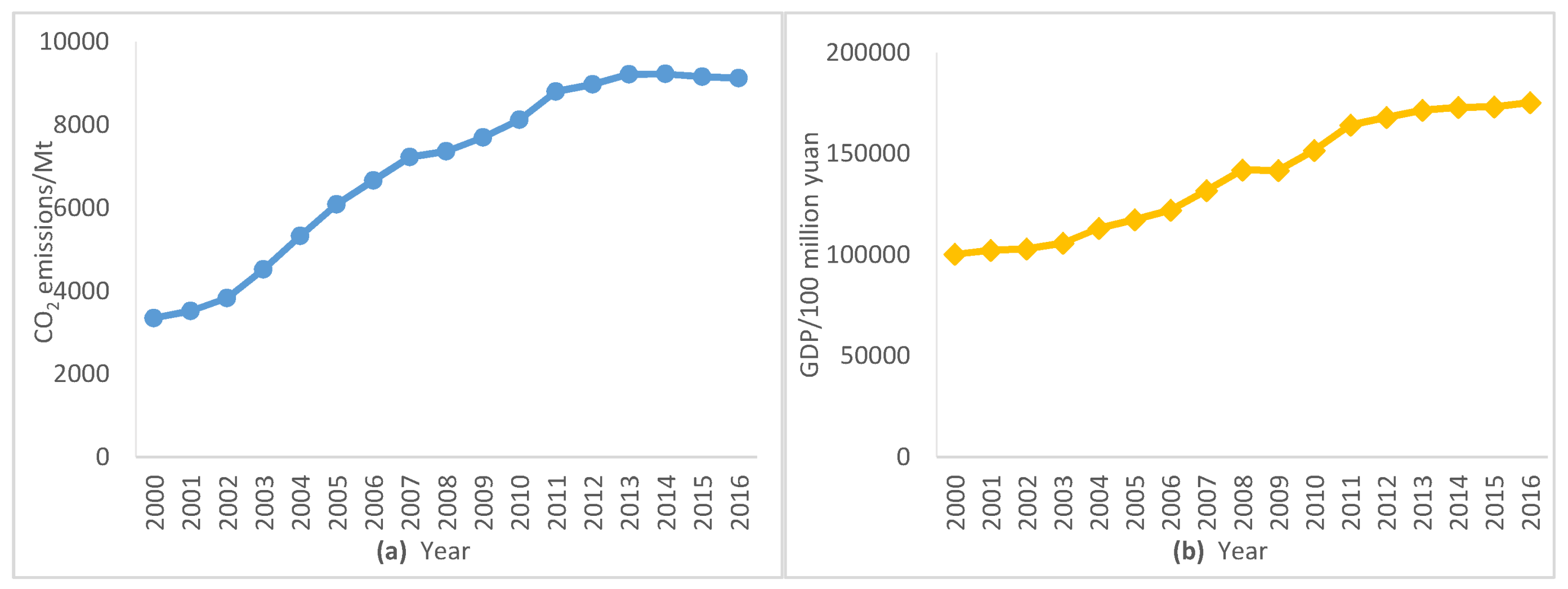
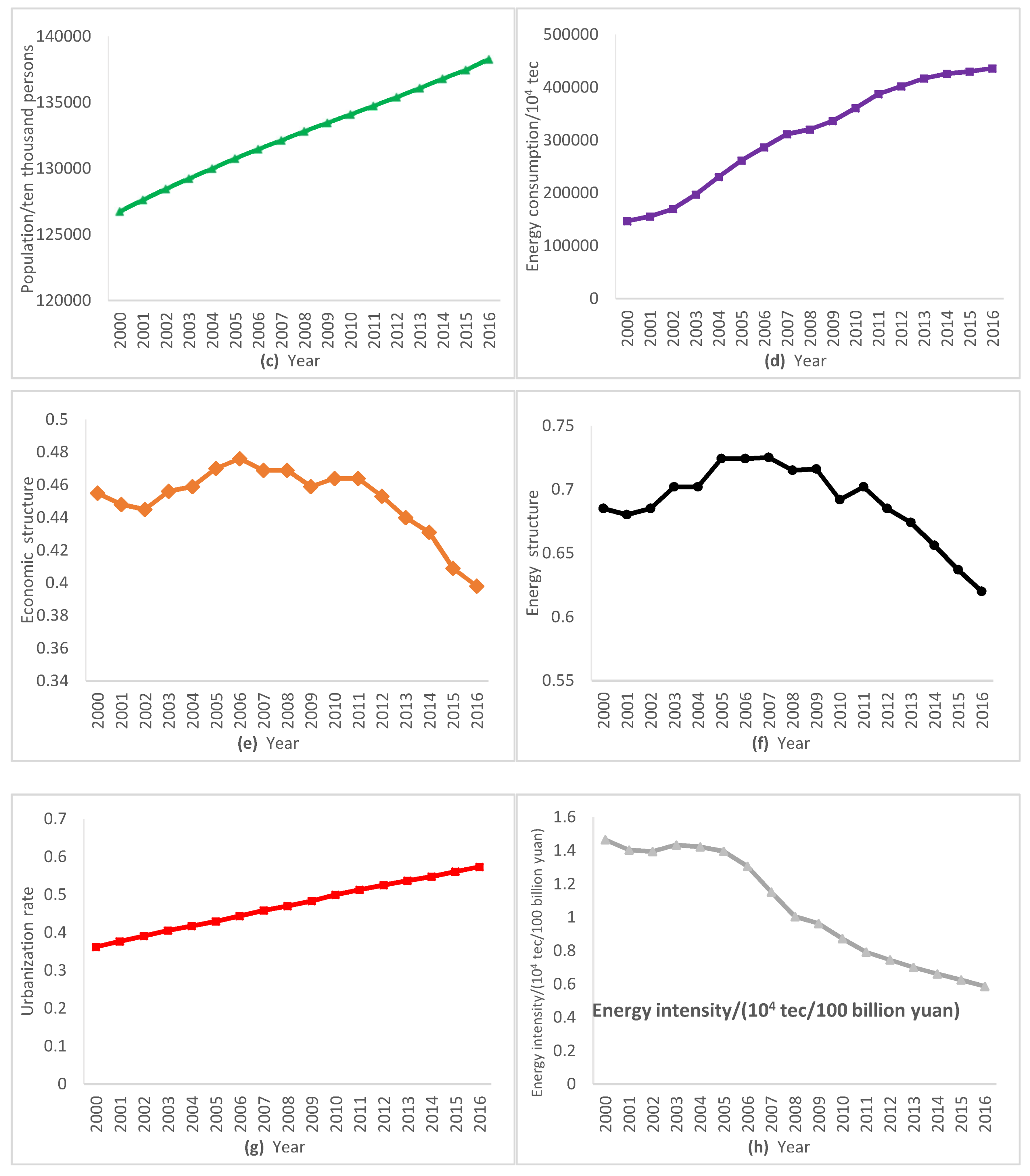
3.1. Data Source and Preprocessing of Data Samples

The SSA-LSSVM method is utilized to forecast the CO2 emissions in China. It is of crucial importance to study the factors that affect CO2 emissions before forecasting, which should be regarded as the input variables in the new proposed model. The relationships of CO2 emissions and their key drivers are nonlinear and complicated. As suggested by the existing research [8,16,24,26,28,30], GDP, population, energy consumption, economic structure, energy structure, urbanization rate, and energy intensity are considered as the major contributors to CO2 emissions in this paper. The economic development, population growth and increased urbanization drive the growth of energy consumption, which leads to increases in CO2 emissions. Economic structure and energy structure affect CO2 emissions by affecting fossil energy consumption. Energy intensity is a manifestation of energy consumption technology affecting CO2 emissions. Further, a correlation analysis is conducted to quantitatively analyze the relationship between CO2 and each factor in this paper, and results are shown in Table 1. All P values are less than 0.05, and the null hypothesis is rejected. Therefore, all selected factors will significantly affect CO2 emissions. GDP, population, energy consumption and urbanization are positively correlated with CO2 emissions. The correlation coefficient between GDP and CO2 emissions is 0.992, which means that economic development is the key factor affecting the increase in CO2 emissions. Economic structure, energy structure, and energy intensity are negatively correlated with CO2 emissions; energy intensity is most strongly related to the decrease in CO2 emissions, followed by energy structure and economic structure. Therefore, all above factors are selected as the input variables for the SSA-LSSVM model.
The data of China’s total CO2 emissions related to energy consumption from 2000 to 2016 are selected from the British Petroleum Statistical Review of World Energy, which presents various energy consumption data that are objective and precise, such as petroleum, coal, natural gas, solar energy and so on. The data on GDP, population, energy consumption, economic structure, energy consumption structure, urbanization rate, and energy intensity from 2000–2016 are picked out from the China Statistical Yearbook. GDP is converted into a constant price by taking 2000 as the base period. Since coal is the most important energy consumer product in China, and the main source of CO2 emissions growth, as suggested by Zheng Wang [27], and Shibao lu [28], the share of coal consumption in total energy consumption indicates the energy consumption structure. China is still an industrialized country dominated by secondary industry, and secondary industry development affects CO2 emissions significantly, according to Zhang X [25] and PhilipKofi Adom [26]. The economic structure is represented by the proportion of the secondary industry added value in terms of GDP.
The data of CO2 emissions, GDP, population, energy consumption, economic structure, energy structure, urbanization rate, and energy intensity in China are shown in Figure 3. The amount of CO2 emitted continuously increased at an average annual rate of 419 million tonnes from 2000 to 2013. After 2011, the growth of CO2 emissions greatly slowed down; China emitted 8979.4 and 9218.8 million tonnes CO2 in 2012 and 2013, respectively. CO2 emissions in 2014 increased by only 5.3 million tonnes compared with 2013, and decreased slightly in 2015–2016 mainly due to the adjustment of industrial structure and energy structure policies. GDP and energy consumption showed the same trend as CO2 emissions, and both have slowed since 2011. The trends of economic structure, energy structure fluctuated from 2000 to 2011, and showed a rapid decline after 2011. In particular, the coal consumption of China has been declining year by year since 2013. Energy intensity has continued to decrease. Population and urbanization both increased stably.
The sample data are normalized, ranging from 0 to 1 by employing Equation (19) before forecasting.
z = x x min x max x min
where x max and x min are the respective maximal and minimal value of each factor data series.
Data samples are divided into a training set and testing set in the use of LSSVM. In this paper, the data of CO2 emissions and driving factors from 2000 to 2013 are selected as the training set; therefore, the sample points of the testing set range from 2014 to 2016.

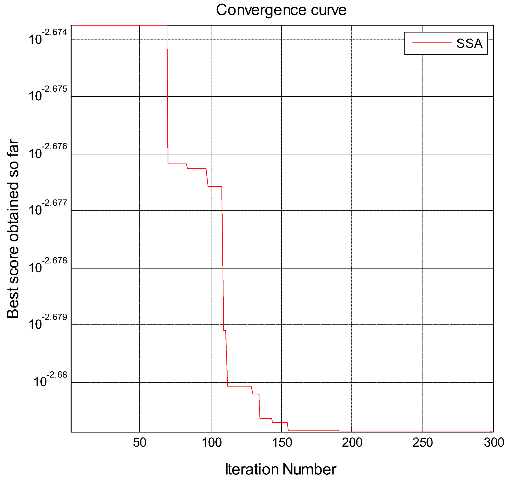
3.2. Optimize LSSVM Parameters and Predict CO2 Emissions

In the SSA-LSSVM model, the values of “ σ 2 ” and “ c ” in the LSSVM model are obtained by the SSA method. The iterative mean absolute error (MAE) tendency of the SSA-LSSVM model results of the optimized parameters is shown as Figure 4. The best optimal value of MAE found by SSA is 0.0020851. The optimal value of “ σ 2 ” is 1546.396, the optimal value of “ c ” is 1,079,561.329, and the two optimal parameters will be applied for CO2 emissions forecasting in the testing stage.
Inputting the data of CO2 factors, the CO2 emissions from 2014 to 2016 can be forecast by the SSA-LSSVM model. The forecasting values are shown in Table 2; the errors between actual CO2 emissions values and forecasting values are extremely small, the gaps between actual values and forecasting values in 2014 and 2015 are −10.399 and 12.158 million tonnes, respectively, the gap in 2016 is only 1.352 million tonnes. Therefore, the proposed SSA-LSSVM model is very accurate.

3.3. Forecasting Performance Evaluation

In order to evaluate the forecasting accuracy of the SSA-LSSVM model and analyze the prediction data of different methods, another three compared methods of prediction are chosen, which are the single LSSVM model, PSO-LSSVM model, and BP neural network model. For the PSO-LSSVM model, the original parameters of PSO are as follows: maxgen = 500, sizepop = 50, Vmax = 10, Vmin = −10, popmax = 10,000,000, popmin = 10. For the BP neural network model, the original parameters are as follows: net.trainparam.lr = 0.1, net.trainparam.epochs = 3000, net.trainparam.goal = 0.0001; the number of hidden neurons is 5. The training set and testing set of the selected models are same as the SSA-LSSVM model, the data between 2000 and 2013 are set as the training set, and the testing set ranges from 2014 to 2016. All factors of CO2 emissions are regarded as the input variables, and CO2 emissions are regarded as output in the forecasting process by the three selected methods.
The actual values and forecasting values of CO2 in China by utilizing the SSA-LSSVM model, PSO-LSSVM model, single LSSVM model, and BP neural network model from 2014–2016 are illustrated in Figure 5. In 2014, the forecasting value of LSSVM has the smallest gap compared with actual value, and the SSA-LSSVM model ranks second. In 2015 and 2016, the SSA-LSSVM model performs best for CO2 emissions compared with other three models, followed by the BP neural network model, PSO-LSSVM model, and LSSVM model.
In order to more directly compare the prediction accuracy of various methods, percentage error (PE), root mean square error (RMSE) and mean absolute percentage error (MAPE) are used to compare and analyze the prediction data of the four models. Their calculation method is shown as below Equations (20)–(22).
P E = x ( k ) x ^ ( k ) x ( k ) × 100 %
R M S E = 1 n k = 1 n ( x ( k ) x ^ ( k ) ) 2
M A P E = 1 n k = 1 n | x ( k ) x ^ ( k ) x ( k ) | × 100 %
where x ( k ) and x ^ ( k ) represent the actual value and the predicted value, respectively, at the time k .
The results of PE, RMSE, and MAPE by different models are demonstrated in Figure 6 and Table 3. Generally, the values of PE ranging in the interval of [−3%, 3%] are considered as standard performance of prediction accuracy [68]. As displayed in Figure 6, all PE values are in the range of the [−3%, 3%] expected prediction point of the LSSVM method in 2016. In particular, the predicted PE values of the SSA-LSSVM model are all in the interval of [−0.2%, 0.2%], which means the proposed SSA-LSSVM model has the best CO2 emissions forecasting performance from 2014 to 2016 based on the PE standard. The gaps between actual values and forecasting values are very small. Therefore, the SSA-LSSVM model has a better prediction performance with respect to CO2 emissions compared with the LSSVM, PSO-LSSVM and BP neural network models.
The results calculated according to RMSE and MAPE also verify the superiority of the SSA-LSSVM model. The RMSE value of the SSA-LSSVM model is 9.27 Mt, which is the smallest compared with other models (203.223 Mt of the LSSVM model, 129.209 Mt of the PSO-LSSVM model, and 79.46 Mt of the BP neural network model). For the MAPE value, SSA-LSSVM is only 0.087%, which is superior to the LSSVM model, PSO-LSSVM model, and BP neural network model with 1.781%, 1.276% and 0.786%, respectively.
Therefore, the proposed SSA-LSSVM model has the best prediction accuracy compared with the LSSVM model, PSO-LSSVM model, and BP neural network model based on the PE, RMSE, and MAPE standard. It can be concluded that the SSA has a better capacity to optimize the parameters of LSSVM with a widely used prospect, and the SSA-LSSVM model has a high accuracy of CO2 emissions forecasting in China, which is significantly superior to the LSSVM model, PSO-LSSVM model, and BP neural network model.

4. Forecasting CO2 Emissions from 2017 to 2020 in China

China’s CO2 emissions from 2017 to 2020 can be forecast by the proposed SSA-LSSVM model. All the factors of CO2 emissions are regarded as input variables in the SSA-LSSVM model; therefore, GDP, population, energy consumption, economic structure, energy structure, urbanization rate, and energy intensity should be forecast from 2017 to 2020. According to the 13th Five-Year Plan for National Economic and Social Development, by 2020, GDP will increase at a steady 6.5% growth rate. The added value of the secondary industry will account for 36.2% of the total output value. The urbanization rate will reach 60%, a total increase of 3.9%. According to the 13th Five-Year Plan for Energy Development, by 2020, the total energy consumption will be controlled at 5 billion tons of standard coal, and the proportion of coal consumption will drop below 58%, and energy intensity will decrease by 15%. The National Plan for the Development of Family Planning in the 13th Five-Year Plan proposes that the total population of the country will be about 1.42 billion at an average annual natural growth rate of about 6% by 2020. The forecasting values of all factors are listed in Table 4.
CO2 emissions in China from 2017 to 2020 can be forecast by the SSA-LSSVM model by using the predicted values of all input variables, and the results are displayed in Figure 7. The CO2 emissions forecasting value in 2017 is 9381.457 million tonnes, and CO2 emissions will reach 10,110.101 million tonnes by 2020. The average annual growth of CO2 emissions is 242.882 Mt, which is much smaller compared with the average growth rate of 2000–2013.
Many scholars have already forecast CO2 emissions of China in 2020: Song Ding [52] utilized an improved GM(1,N) model to forecast CO2 emissions, Lu Xing [69] forecast CO2 emissions by constructing a Leap model, and Zhang Chuanping [70] calculated the CO2 emissions according to the emissions target proposed by the State Council. The above three forecasting values of CO2 emissions are shown in Table 5. The CO2 emissions forecasting value of this paper is less than the three other forecasting values. Structural factors should be considered in the CO2 emissions forecasting process as these are frequently overlooked in some research, leading to a higher forecasting value of CO2 emissions. The proposed model in this paper can contribute to improving the CO2 emissions forecasting accuracy, and the forecasting result may guide the Chinese government to formulate more reasonable CO2 emission reduction policies. The impact on CO2 emissions of structural factors is significant; therefore, it is necessary to design stronger, more critical and more scientific energy structural and economic structurale development policies.
The growing speed slows down because of a series of policies and actions taken by the Chinese government, such as industrial restructuring policy, energy structure adjustment policy, and eco-friendly development policy, and so on. In particular, China proposed the “two alternative” energy consumption strategy, which contributes to the change of energy structure and vigorously develops clean energy. China invested US$ 89.5 billion in clean energy according to the data in 2014 from the National Bureau of Statistics of China, accounting for 29% of total investment in global renewable development. Recently, China has focused on continuously cutting overcapacity of some key industries including steel and cement; the development of these industries requires a large amount of fossil energy consumption, which is the main source of CO2 emissions. Therefore, the implementation of the capacity policy is conducive to promoting the adjustment of industrial structure and energy structure, and reducing the CO2 emissions in China. Strategies of “Made in China 2025” and “Industry 4.0” also upgrade the industrial structure of China. All policies and actions help China achieve its emission reduction targets.
The constant decrease in emissions growth means the peak of China’s CO2 emissions is coming. In the future, China will further stabilize its economic development, optimize the energy structure and industrial structure, increase the implementation of energy conservation and emission reduction policies, and strictly control the total amount of energy consumption and pollutant emissions. It is entirely possible to reach a peak by 2030 in accordance with the current development trend.

5. Conclusions

CO2 emissions forecasting is becoming more important due to increasing climatic problems and contributes to developing scientific climate policies and making reasonable energy plans. Considering that the influential factors of CO2 emissions are multiplex, and the relationship between each factor and CO2 emissions is complex and non-linear, CO2 emissions forecasting is also difficult, which is worth further study. In this paper, a novel CO2 emissions forecasting model is proposed based on the LSSVM model, which is widely used to solve complex and non-linear problems, and the SSA method, which has superiority in solving single-objective optimization problems with unknown search spaces compared with the general optimization algorithm, namely, the SSA-LSSVM model. GDP, population, energy consumption, economic structure, energy structure, urbanization rate, and energy intensity are all found to affect CO2 emissions in some context based on a summary of previous research. Moreover, it is found that GDP, population, energy consumption and urbanization are positively correlated with CO2 emissions, and economic structure, energy structure, and energy intensity are negatively correlated with CO2 emissions by correlation analysis. Therefore, all factors are considered as input variables in the SSA-LSSVM model; in particular, the structural factors are considered in the CO2 emissions forecasting process. However, the impact on CO2 emissions of carbon capture technology is not considered due to the difficulty of quantifying it in the proposed model in this paper. The proposed SSA-LSSVM model is verified to have superiority and better performance in terms of CO2 emissions forecasting compared with the selected models, including the single LSSVM model, PSO-LSSVM model, BP neural network model, based on three different evaluation indicators, namely, PE, RMSE, and MAPE. The predicted PE values of the SSA-LSSVM model are all in the interval of [−0.2%, 0.2%], the RMSE value of the SSA-LSSVM model is 9.27 Mt, and the MAPE value of the SSA-LSSVM model is only 0.087%. Therefore, the SSA-LSSVM model can improve the accuracy and reliability of CO2 emissions forecasting. CO2 emissions will reach 10,110.101 Mt by 2020 in China, forecast by the SSA-LSSVM model according to the 13th Five-Year Plan for social, economic and energy development, and the average annual growth is 242.882 Mt, i.e., considerably lower compared to the growth from 2000 to 2013. The CO2 emissions forecasting value of China in 2020 in this paper is less than the three other forecasting values, which indicates that structural factors should be taken into account in the forecasting process, and ignoring structural factors may lead to higher a forecasting value. Therefore, the proposed model in this paper can improve the accuracy of CO2 emissions forecasting and help the Chinese government to formulate more reasonable CO2 emission reduction policies, energy structure adjustment policies and economic structure transformation policies. The constant decrease of CO2 emissions benefits from a series of policies and actions, such as the industrial restructuring policy, energy structural adjustment policy and the “two alternative” energy consumption strategy. It is entirely possible to reach a peak by 2030 in accordance with the current development trend.
The SSA can be applied to more practical issues combined with other methods, such as the BP neural network, extreme learning machine (ELM), and SVM, which has a better potential for optimization. Considering that the development of influential factors of CO2 emissions is uncertain and changeable, the scenario analysis method could contribute to CO2 emissions forecasting and analysis, which is the focus of further study. Moreover, quantifying the impacts on CO2 emissions of carbon capture technologies in the model may further improve the forecasting accuracy of the SSA-LSSVM model, which is the focus of the next step.

Acknowledgments

This thesis is funded by the National Key R&D Program of China with Grant No. 2016YFB0900501, and the Fundamental Research Funds for the Central Universities, Grant No. 2017MS060 and 2017XS106.

Author Contributions

Huiru Zhao proposed the concept of this study. Guo Huang completed the paper. Ning Yan modified the final draft of the manuscript.

Conflicts of Interest

The authors declare no conflict of interest.

References

  1. Davis, S.J.; Caldeira, K.; Matthews, H.D. Future CO2 emissions and climate change from existing energy infrastructure. Science 2010, 329, 1330–1333. [Google Scholar] [CrossRef] [PubMed]
  2. Dawson, B.; Spannagle, M. United Nations Framework Convention on Climate Change (UNFCCC). Complet. Guide Clim. Chang. 2010, 10, 227–239. [Google Scholar]
  3. British Petroleum Statistical Review of World Energy. 2017. Available online: https://www.bp.com/zh_cn/china/reports-and-publications/_bp_2017-_.html (accessed on 2 January 2018).
  4. Global Carbon Atlas. 2016. Available online: http://www.globalcarbonatlas.org/cn/CO2-emissions (accessed on 2 January 2018).
  5. Yang, L. Industry 4.0: A survey on technologies, applications and open research issues. J. Ind. Inf. Integr. 2017, 6, 1–10. [Google Scholar]
  6. Meng, F.; Su, B.; Thomson, E.; Zhou, D.; Zhou, P. Measuring China’s regional energy and carbon emission efficiency with DEA models: A survey. Appl. Energy 2016, 183, 1–21. [Google Scholar] [CrossRef]
  7. Zhao, H.; Guo, S.; Zhao, H. Energy-Related CO2 Emissions Forecasting Using an Improved LSSVM Model Optimized by Whale Optimization Algorithm. Energies 2017, 10, 874. [Google Scholar] [CrossRef]
  8. Saboori, B.; Sulaiman, J. CO2, emissions, energy consumption and economic growth in Association of Southeast Asian Nations (ASEAN) countries: Acointegration approach. Energy 2013, 55, 813–822. [Google Scholar] [CrossRef]
  9. Arouri, M.E.H.; Youssef, A.B.; M’Henni, H.; Rault, C. Energy consumption, economic growth and CO2, emissions in Middle East and North African countries. Energy Policy 2012, 45, 342–349. [Google Scholar] [CrossRef] [Green Version]
  10. Ang, J.B. CO2 emissions, energy consumption, and output in France. Energy Policy 2007, 35, 4772–4778. [Google Scholar] [CrossRef]
  11. Soytas, U.; Sari, R.; Ewing, B.T. Energy consumption, income, and carbon emissions in the United States. Ecol. Econ. 2007, 62, 482–489. [Google Scholar] [CrossRef]
  12. Zhang, X.P.; Cheng, X.M. Energy consumption, carbon emissions, and economic growth in China. Ecol. Econ. 2009, 68, 2706–2712. [Google Scholar] [CrossRef]
  13. Ghosh, S. Examining carbon emissions economic growth nexus for India: A multivariate cointegration approach. Energy Policy 2010, 38, 3008–3014. [Google Scholar] [CrossRef]
  14. Lotfalipour, M.R.; Falahi, M.A.; Ashena, M. Economic growth, CO2, emissions, and fossil fuels consumption in Iran. Energy 2010, 35, 5115–5120. [Google Scholar] [CrossRef]
  15. Ilhan, O.; Ali, A. CO2 emissions, energy consumption and economic growth in Turkey. Renew. Sustain. Energy Rev. 2010, 14, 3220–3225. [Google Scholar]
  16. Knapp, T.; Mookerjee, R. Population growth and global CO2, emissions: A secular perspective. Energy Policy 2007, 24, 31–37. [Google Scholar] [CrossRef]
  17. Zhu, Q.; Peng, X. The impacts of population change on carbon emissions in China during 1978–2008. Environ. Impact Assess. Rev. 2012, 36, 1–8. [Google Scholar] [CrossRef]
  18. Wang, Z.; Yin, F.; Zhang, Y.; Zhang, X. An empirical research on the influencing factors of regional CO2, emissions: Evidence from Beijing city, China. Appl. Energy 2012, 100, 277–284. [Google Scholar] [CrossRef]
  19. Wang, P.; Wu, W.; Zhu, B.; Wei, Y. Examining the impact factors of energy-related CO2, emissions using the STIRPAT model in Guangdong Province, China. Appl. Energy 2013, 106, 65–71. [Google Scholar] [CrossRef]
  20. Wang, Y.; Zhao, T. Impacts of energy-related CO2, emissions: Evidence from under developed, developing and highly developed regions in China. Ecol. Indic. 2015, 50, 186–195. [Google Scholar] [CrossRef]
  21. Cole, M.A.; Neumayer, E. Examining the Impact of Demographic Factors on Air Pollution. Popul. Environ. 2004, 26, 5–21. [Google Scholar] [CrossRef]
  22. Liddle, B.; Nelson, D.R. Age-structure, urbanization, and climate change in developed countries: Revisiting STIRPAT for disaggregated population and consumption-related environmental impacts. Popul. Environ. 2010, 31, 317–343. [Google Scholar] [CrossRef]
  23. Fan, Y.; Liu, L.C.; Wu, G.; Wei, Y.M. Analyzing impact factors of CO2, emissions using the STIRPAT model. Environ. Impact Assess. Rev. 2006, 26, 377–395. [Google Scholar] [CrossRef]
  24. Maruotti, A. The impact of urbanization on CO2 emissions: Evidence from developing countries. Ecol. Econ. 2011, 70, 1344–1353. [Google Scholar]
  25. Zhang, X.; Ren, J. The Relationship between Carbon Dioxide Emissions and Industrial Structure Adjustment for Shandong Province. Energy Procedia 2011, 5, 1121–1125. [Google Scholar]
  26. Adom, P.K.; Bekoe, W.; Amuakwa-Mensah, F.; Mensah, J.T.; Botchway, E. Carbon dioxide emissions, economic growth, industrial structure, and technical efficiency: Empirical evidence from Ghana, Senegal, and Morocco on the causal dynamics. Energy 2012, 47, 314–325. [Google Scholar] [CrossRef]
  27. Wang, Z.; Zhu, Y.; Zhu, Y.; Shi, Y. Energy structure change and carbon emission trends in China. Energy 2016, 115, 369–377. [Google Scholar] [CrossRef]
  28. Lu, S.; Wang, J.; Shang, Y.; Bao, H.; Chen, H. Potential assessment of optimizing energy structure in the city of carbon intensity target. Appl. Energy 2016, 194, 765–773. [Google Scholar] [CrossRef]
  29. Shahbaz, M. Multivariate Granger Causality between CO2 Emissions, Energy Intensity, Financial Development and Economic Growth: Evidence from Portugal; University Library of Munich: Munich, Germany, 2012. [Google Scholar]
  30. Lin, B.; Liu, K. Using LMDI to Analyze the Decoupling of Carbon Dioxide Emissions from China’s Heavy Industry. Sustainability 2017, 9, 1198–1203. [Google Scholar]
  31. Ma, M.; Shen, L.; Ren, H.; Cai, W.; Ma, Z. How to Measure Carbon Emission Reduction in China’s Public Building Sector: Retrospective Decomposition Analysis Based on STIRPAT Model in 2000–2015. Sustainability 2017, 9, 1744. [Google Scholar] [CrossRef]
  32. Wu, R.; Zhang, J.; Bao, Y.; Lai, Q.; Tong, S.; Song, Y. Decomposing the Influencing Factors of Industrial Sector Carbon Dioxide Emissions in Inner Mongolia Based on the LMDI Method. Sustainability 2016, 8, 661. [Google Scholar] [CrossRef]
  33. Coninck, H.D.; Loos, M.A.; Metz, B.; Davidson, O.; Meyer, L. IPCC Special Report on Carbon Dioxide Capture and Storage; Intergovernmental Panel on Climate Change: Geneva, Switzerland, 2005. [Google Scholar]
  34. Budzianowski, W.M. Negative carbon intensity of renewable energy technologies involving biomass or carbon dioxide as inputs. Renew. Sustain. Energy Rev. 2012, 16, 6507–6521. [Google Scholar] [CrossRef]
  35. Safdarnejad, S.M.; Hedengren, J.D.; Baxter, L.L. Dynamic optimization of a hybrid system of energy-storing cryogenic carbon capture and a baseline power generation unit. Appl. Energy 2016, 172, 66–79. [Google Scholar] [CrossRef]
  36. Safdarnejad, S.M.; Hedengren, J.D.; Baxter, L.L. Plant-level dynamic optimization of Cryogenic Carbon Capture with conventional and renewable power sources. Appl. Energy 2015, 149, 354–366. [Google Scholar] [CrossRef]
  37. Kang, C.A.; Brandt, A.R.; Durlofsky, L.J. Optimizing heat integration in a flexible coal–natural gas power station with CO2, capture. Int. J. Greenh. Gas Control 2014, 31, 138–152. [Google Scholar] [CrossRef]
  38. Gopan, A.; Kumfer, B.M.; Phillips, J.; Thimsen, D.; Smith, R.; Axelbaum, R.L. Process design and performance analysis of a Staged, Pressurized Oxy-Combustion (SPOC) power plant for carbon capture. Appl. Energy 2014, 125, 179–188. [Google Scholar] [CrossRef]
  39. Belaissaoui, B.; Cabot, G.; Cabot, M.S.; Willson, D.; Favre, E. CO2 capture for gas turbines: An integrated energy-efficient process combining combustion in oxygen-enriched air, flue gas recirculation, and membrane separation. Chem. Eng. Sci. 2013, 97, 256–263. [Google Scholar] [CrossRef]
  40. Gazzani, M.; Turi, D.M.; Ghoniem, A.F.; Macchi, E.; Manzolini, G. Techno-economic assessment of two novel feeding systems for a dry-feed gasifier in an IGCC plant with Pd-membranes for CO2, capture. Int. J. Greenh. Gas Control 2014, 25, 62–78. [Google Scholar] [CrossRef]
  41. Rezakazemi, M.; Amooghin, A.E.; Montazer-Rahmati, M.M.; Ismail, A.F.; Matsuura, T. State-of-the-art membrane based CO2, separation using mixed matrix membranes (MMMs): An overview on current status and future directions. Prog. Polym. Sci. 2014, 39, 817–861. [Google Scholar] [CrossRef]
  42. Burnett, J.W.; Bergstrom, J.C.; Dorfman, J.H. A spatial panel data approach to estimating U.S. state-level energy emissions. Energy Econ. 2013, 40, 396–404. [Google Scholar] [CrossRef]
  43. Talbi, B. CO2 emissions reduction in road transport sector in Tunisia. Renew. Sustain. Energy Rev. 2017, 69, 232–238. [Google Scholar] [CrossRef]
  44. Ahmed, K. Environmental Kuznets Curve and Pakistan: An Empirical Analysis. Procedia Econ. Finance 2012, 1, 4–13. [Google Scholar] [CrossRef]
  45. Kumar, S.; Madlener, R. CO2 emission reduction potential assessment using renewable energy in India. Energy 2016, 97, 273–282. [Google Scholar] [CrossRef]
  46. Liu, Y.Y.; Wang, Y.F.; Yang, J.Q.; Zhou, Y. Scenario Analysis of Carbon Emissions in Jiangxi Transportation Industry Based on LEAP Model. Appl. Mech. Mater. 2011, 66–68, 637–642. [Google Scholar] [CrossRef]
  47. Chang, Z.; Pan, K.X. An Analysis of Shanghai’s Long-Term Energy Consumption and Carbon Emission Based on LEAP Model. Contemp. Finance Econ. 2014, 1079–1080, 502–505. [Google Scholar]
  48. Li, J.; Shi, J.; Li, J. Exploring Reduction Potential of Carbon Intensity Based on Back Propagation Neural Network and Scenario Analysis: A Case of Beijing, China. Energies 2016, 9, 615. [Google Scholar] [CrossRef]
  49. Liang, Q.M.; Fan, Y.; Wei, Y.M. Multi-regional input–output model for regional energy requirements and CO2 emissions in China. Energy Policy 2007, 35, 1685–1700. [Google Scholar] [CrossRef]
  50. Lin, C.S.; Liou, F.M.; Huang, C.P. Gray forecasting model for CO2 emissions: A Taiwan study. Appl. Energy 2011, 88, 3816–3820. [Google Scholar] [CrossRef]
  51. Pao, H.T.; Tsai, C.M. Modeling and forecasting the CO2, emissions, energy consumption, and economic growth in Brazil. Energy 2011, 36, 2450–2458. [Google Scholar] [CrossRef]
  52. Ding, S.; Dang, Y.G.; Li, X.M.; Wang, J.J.; Zhao, K. Forecasting Chinese CO2, emissions from fuel combustion using a novel gray multivariable model. J. Clean. Prod. 2017, 162, 1527–1538. [Google Scholar] [CrossRef]
  53. Pao, H.T.; Fu, H.C.; Tseng, C.L. Forecasting of CO2, emissions, energy consumption and economic growth in China using an improved gray model. Energy 2012, 40, 400–409. [Google Scholar] [CrossRef]
  54. Yao, T.; Liu, S.; Xie, N. On the properties of small sample of GM(1,1) model. Appl. Math. Model. 2009, 33, 1894–1903. [Google Scholar] [CrossRef]
  55. Niu, D.; Dai, S. A Short-Term Load Forecasting Model with a Modified Particle Swarm Optimization Algorithm and Least Squares Support Vector Machine Based on the Denoising Method of Empirical Mode Decomposition and Grey Relational Analysis. Energies 2017, 10, 408. [Google Scholar] [CrossRef]
  56. Guo, W.; Zhao, Z. A novel hybrid BND-FOA-LSSVM model for electricity price forecasting. Information 2017, 8, 120. [Google Scholar]
  57. Wu, Q.; Peng, C. A Least Squares Support Vector Machine Optimized by Cloud-Based Evolutionary Algorithm for Wind Power Generation Prediction. Energies 2016, 9, 585. [Google Scholar] [CrossRef]
  58. Sun, W.; Sun, J. Daily PM2.5 concentration prediction based on principal component analysis and LSSVM optimized by cuckoo search algorithm. J. Environ. Manag. 2017, 188, 144–152. [Google Scholar] [CrossRef] [PubMed]
  59. Li, H.; Guo, S.; Zhao, H.; Su, C.; Wang, B. Annual Electric Load Forecasting by a Least Squares Support Vector Machine with a Fruit Fly Optimization Algorithm. Energies 2012, 5, 4430–4445. [Google Scholar] [CrossRef]
  60. Li, J.; Zhang, B.; Shi, J. Combining a Genetic Algorithm and Support Vector Machine to Study the Factors Influencing CO2 Emissions in Beijing with Scenario Analysis. Energies 2017, 10, 1520. [Google Scholar] [CrossRef]
  61. Sulaiman, M.H.; Mustafa, M.W.; Shareef, H.; Khalid, S.N.A. An application of artificial bee colony algorithm with least squares support vector machine for real and reactive power tracing in deregulated power system. Int. J. Electr. Power Energy Syst. 2012, 37, 67–77. [Google Scholar] [CrossRef]
  62. Mirjalili, S.; Gandomi, A.H.; Mirjalili, S.Z.; Saremi, S.; Faris, H.; Mirjalili, S.M. Salp Swarm Algorithm: A bio-inspired optimizer for engineering design problems. Adv. Eng. Softw. 2017, 114, 163–191. [Google Scholar] [CrossRef]
  63. Miranian, A.; Abdollahzade, M. Developing a local least-squares support vector machines-based neuro-fuzzy model for nonlinear and chaotic time series prediction. IEEE Trans. Neural Netw. Learn. Syst. 2013, 24, 207–218. [Google Scholar] [CrossRef] [PubMed]
  64. Cao, L.J.; Tay, F.H. Support vector machine with adaptive parameters in financial time series forecasting. IEEE Trans. Neural Netw. 2003, 14, 1506–1518. [Google Scholar] [CrossRef] [PubMed]
  65. Gryllias, K.C.; Antoniadis, I.A. A Support Vector Machine approach based on physical model training for rolling element bearing fault detection in industrial environments. Eng. Appl. Artif. Intell. 2012, 25, 326–344. [Google Scholar] [CrossRef]
  66. Madin, L.P. Aspects of jet propulsion in salps. Can. J. Zool. 1990, 68, 765–777. [Google Scholar] [CrossRef]
  67. Anderson, P.A.V.; Bone, Q. Communication between Individuals in Salp Chains II. Physiology. Proc. R. Soc. Lond. 1980, 210, 559–574. [Google Scholar] [CrossRef]
  68. Amiri, M.; Davande, H.; Sadeghian, A.; Chartier, S. Feedback associative memory based on a new hybrid model of generalized regression and self-feedback neural networks. Neural Netw. 2010, 23, 892–904. [Google Scholar] [CrossRef] [PubMed]
  69. Xing, L.; Shan, B.; Xu, M.; Shi, L. China’s CO2 Emission Scenarios to Meet the Low Carbon Goals by 2020. Adv. Inf. Sci. Serv. Sci. 2012, 4, 320–326. [Google Scholar]
  70. Zhang, C.; Niu, X.; Zhou, Q. Research on China Energy Structure with CO2 Minimum Emission In 2020. Energy Procedia 2011, 5, 1084–1092. [Google Scholar]
Figure 1. Individual salp and a swarm of salps (salp chain). (a) individual salp; (b) a swarm of salps (salp chain).
Energies 11 00781 g001
Figure 2. The procedure of the SSA-LSSVM model for CO2 emissions forecasting.
Energies 11 00781 g002
Figure 3. The sample data of CO2 emissions and selected factors in China from 2000 to 2016. (a) CO2 emissions; (b) GDP; (c) population; (d) energy consumption; (e) economic structure; (f) energy structure; (g) urbanization; (h) energy intensity.
Energies 11 00781 g003aEnergies 11 00781 g003b
Figure 4. The iterative mean absolute error tendency of the SSA-LSSVM model of the optimized parameters.
Energies 11 00781 g004
Figure 5. Forecasting values of CO2 emissions from 2014 to 2016 in China by different methods.
Energies 11 00781 g005
Figure 6. PE values of four forecasting models.
Energies 11 00781 g006
Figure 7. The predicted CO2 emissions from 2017 to 2020 by SSA-LSSVM.
Energies 11 00781 g007
Table 1. Correlation analysis between CO2 and each factor.
VariablesGDPPopulationEnergy ConsumptionEconomic Structure
CO2Correlation coefficient0.9920.9350.987−0.752
p value0000.0076
VariablesEnergy StructureUrbanizationEnergy Intensity
CO2Correlation coefficient−0.8230.952−0.972
p value0.001900
Table 2. Forecasting values and gaps of CO2 emissions of the SSA-LSSVM model.
YearActual Value (Mt)Forecasting Value (Mt)The Value of Gap * (Mt)
20149224.1029234.501 −10.399
20159164.4539152.295 12.158
20169123.0499121.698 1.352
* The value of gap = the actual value—the forecasting value.
Table 3. RMSE and MAPE values of four forecasting models.
ModelSSA-LSSVMPSO-LSSVMLSSVMBP Neural Network
RMSE (Mt)9.270 129.209 203.223 79.460
MAPE (%)0.0871.2761.7810.786
Table 4. The forecasting values of all factors from 2017 to 2020 in China.
Year2017201820192020
GDP/(100 million yuan)186,687198,821211,745225,508
Population/(104 persons)139,171140,071140,971141,871
Urbanization rate0.5800.5870.5930.600
Energy Consumption/(104 tec)452,000468,000484,000500,000
Economic Structure0.3890.3800.3710.362
Energy Structure0.6100.6000.5900.580
Energy Intensity/(104 tec/100 million yuan)0.5580.5300.5020.474
Table 5. Forecasting values of CO2 emissions of China in 2020 by different methods.
AuthorsS Ding [52] L Xing [69]Zhang C [70]Zhao H
CO2/(Mt)11,002.1510,993.1613,770.1810,110.10

