The Impact of Drive Cycles and Auxiliary Power on Passenger Car Fuel Economy


Abstract
:1. Introduction
1.1. Simulation-Based Fuel Consumption Analysis
- Passenger car characteristics: external parameters specific to vehicle classes;
- Consumers of the on-board power system and their time-dependent load profiles;
- Approaches to scaling drive components;
- Fuel consumption-optimized operating strategies.
1.2. Use of Electrical Power in Passenger Car Drive Concepts
2. Methodology
2.1. Energy Balance and Scaling the Drive Components
2.2. Dynamic Simulation
- Globally-applicable constants;
- Vehicle class-specific parameters; and
- Characteristic values of the model components.
2.3. Optimizing Operating Strategies
- Transmission ratio (gear) for all concepts;
- EM and ICE torque for PAH;
- Fuel cell system power for FCV.
2.4. Fuel Economy Assessment
3. Results and Discussion
4. Conclusions
Author Contributions
Conflicts of Interest
Appendix A

| Acronym | Description | Acronym | Description |
|---|---|---|---|
| AC | Air conditioning | HYZEM | Drive cycle |
| AD | Axle drive | ICE | Internal combustione engine |
| APU | Auxiliary power unit | ICV | Internal combustione engine vehicle |
| ASG | Automated gearbox | LPE | Load point elevation |
| BE | Battery electric | LPR | Load point reduction |
| BEV | Battery electric vehicle | MODEM | Drive cycle |
| BSL | Base load only (load case) | MVEG | European standard driving cycle |
| BT | Battery | NHC | No heating or cooling (load case) |
| CP | Cooling power | OG | 14 V on-board power system |
| CVT | Continuously variable transmission | OPS | Operating point shift |
| DC | DC (direct current) converter | PAH | Parallel hybrid |
| EM | Electric machine | PEFC | Polymer electrolyte fuel cell |
| EUDC | MVEG sub-cycle for extra urban driving | PHEV | Plug-in hybrid |
| EV | Electric vehicle | PSH | Power-split hybrid |
| FCV | Fuel cell vehicle | RC | Resistor capacitor element |
| FLC | Fuzzy logic controller | SEH | Series hybrid |
| FRD | Frost day | SI | Spark ignition |
| FT | Fuel tank | SOC | State of charge |
| FTP | Federal Test Procedure | SUD | Summer day |
| GB | Gear box | SUV | Sports utility vehicle |
| HEV | Hybrid electric vehicle | TTW | Tank-to-wheel |
| HP | Heating power | WLTC | Worldwide harmonized light vehicles test cycles |
| HT | Heating element | WTW | Well-to-wheel |
| HWFET | Highway Fuel Economy Test |
| Drive Cycle Name | Average Velocity | Mechanical Energy at the Wheels | Box Plot of Passenger Car Drive Power (Histogram) |
|---|---|---|---|
| Cycle group “urban” | |||
| ARTEMIS urban | ; |  | |
| ECE |  | ||
| US FTP 72 | 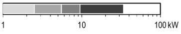 | ||
| HYZEM urban | 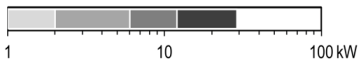 | ||
| Japan 08 | 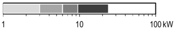 | ||
| MODEM free flow urban | 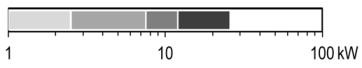 | ||
| MODEM slow urban |  | ||
| SFTP-SC03 | 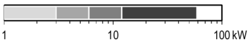 | ||
| WLTC, ver. 4.0 low | 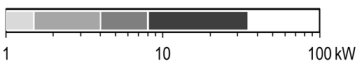 | ||
| WLTC, ver. 4.0 middle | 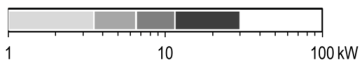 | ||
| Cycle group “Extra urban” | |||
| ARTEMIS road | 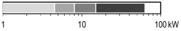 | ||
| EUDC | 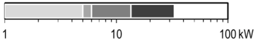 | ||
| HYZEM rural |  | ||
| MODEM road | 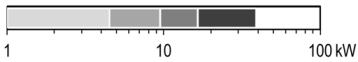 | ||
| SFTP-US06 |  | ||
| WLTC, ver. 4.0 high | 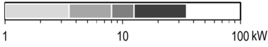 | ||
| Cycle group “Motorway” | |||
| ARTEMIS motorway (130) |  | ||
| US Highway | 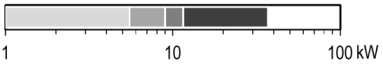 | ||
| HYZEM highway | 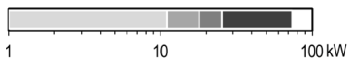 | ||
| MODEM motorway | 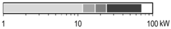 | ||
| WLTC, ver. 4.0 very high | 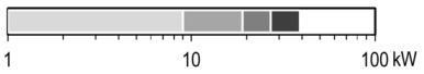 | ||
| Cycle group “Combined“ | |||
| HYZEM | 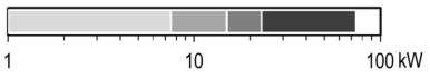 | ||
| MODEM | 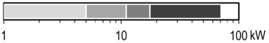 | ||
| MVEG | ; | 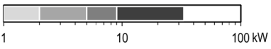 | |
| WLTC, ver. 4.0 | ; | 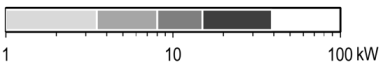 | |
Example histogram (MVEG)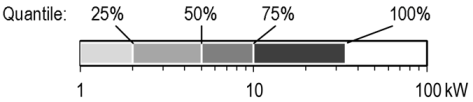 | |||
| Concept | A-Segment | C-Segment | |||||||||||
|---|---|---|---|---|---|---|---|---|---|---|---|---|---|
| “Standard” | “Advanced” | “Standard” | “Advanced” | ||||||||||
| ICV-G | n.a. | n.a. | n.a. | n.a. | |||||||||
| ICV-D | n.a. | n.a. | n.a. | n.a. | |||||||||
| PAH-G | |||||||||||||
| PAH-D | |||||||||||||
| BEV | n.a. | n.a. | n.a. | n.a. | |||||||||
| FCV | n.a. | n.a. | n.a. | n.a. | |||||||||

| A-Segment | C-Segment | |||
|---|---|---|---|---|
| Concept | “Standard” | “Advanced” | “Standard” | “Advanced” |
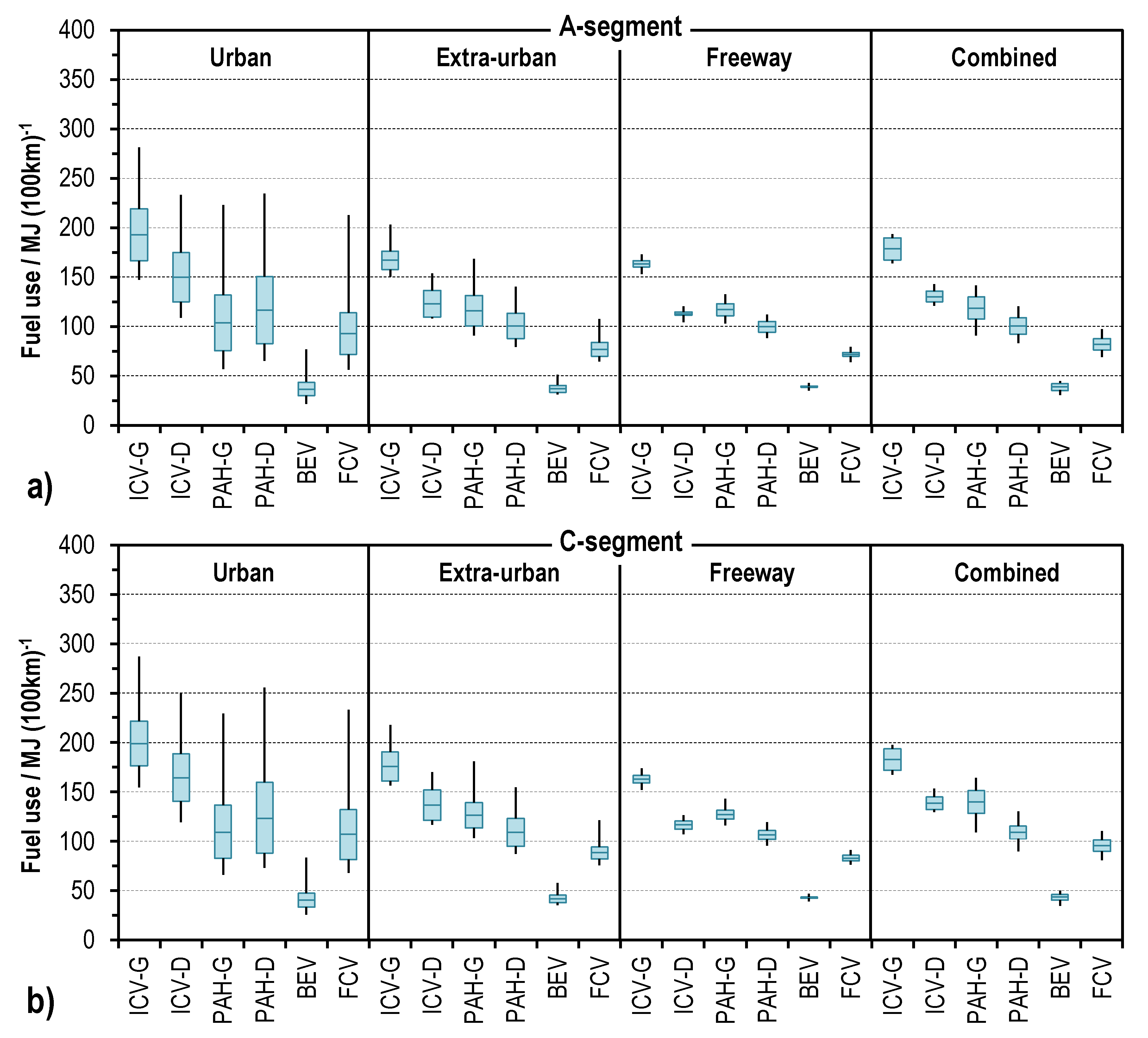
| ICV-G “Base load only” (BSL) | 144–224 | 132–203 | 152–255 | 136–227 |
| 171|154|161 | 159|142|149 | 187|165|174 | 170|147|156 | |
| 167|148|151|165 | 148|132|138|149 | 185|164|162|179 | 162|143|144|157 | |
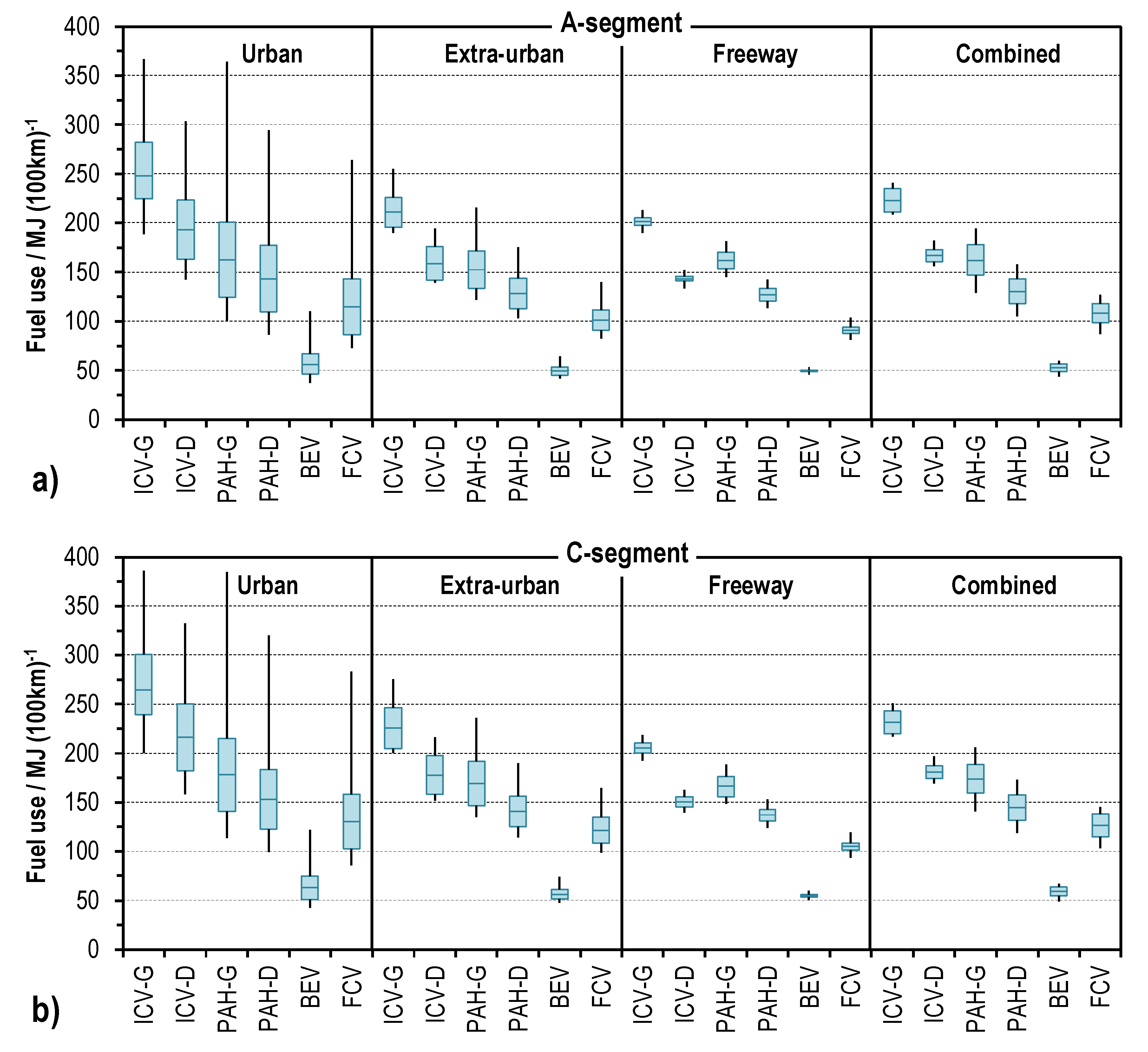
| ICV-G “Frost day” (FRD) | 154–300 | 143–270 | 161–325 | 144–288 |
| 225|167|189 | 203|154|172 | 243|178|202 | 216|159|180 | |
| 233|171|166|186 | 211|153|152|169 | 250|186|177|199 | 222|162|157|176 | |
| ICV-G “No heating & cooling” (NHC) | 153–282 | 142–255 | 160–303 | 144–270 |
| 210|165|182 | 192|152|167 | 226|176|195 | 203|157|174 | |
| 224|167|164|183 | 202|150|150|166 | 238|181|175|196 | 211|158|155|173 | |
| ICV-D “Baseload only” (BSL) | 104–183 | 103–176 | 113–215 | 106–202 |
| 136|113|122 | 137|110|120 | 156|126|138 | 154|117|131 | |
| 134|113|112|125 | 130|106|109|120 | 154|130|125|141 | 145|119|116|129 | |
| ICV-D “Frost day” (FRD) | 112–251 | 110–240 | 121–280 | 113–261 |
| 184|125|147 | 176|120|141 | 206|138|163 | 195|127|152 | |
| 190|133|126|143 | 184|125|121|137 | 211|151|139|159 | 197|137|128|146 | |
| ICV-D “No heating & cooling” (NHC) | 112–228 | 110–222 | 121–252 | 112–239 |
| 168|123|140 | 164|118|136 | 187|136|155 | 181|125|146 | |
| 176|128|123|139 | 174|121|119|134 | 194|144|136|154 | 185|132|125|142 | |
| A-Segment | C-Segment | |||
|---|---|---|---|---|
| Concept | “Standard” | “Advanced” | “Standard” | “Advanced” |
| PAH-G “Baseload only” (BSL) | 90–177 | 65–152 | 102–195 | 72–165 |
| 105|129|119 | 83|108|99 | 114|139|130 | 90|115|106 | |
| 90|96|116|125 | 65|73|94|103 | 102|107|129|140 | 72|84|105|113 | |
| PAH-G “Frost day” (FRD) | 145–322 | 116–245 | 158–351 | 124–260 |
| 229|157|185 | 186|131|152 | 251|169|200 | 198|138|161 | |
| 226|147|151|171 | 173|116|124|140 | 244|161|163|185 | 186|124|131|150 | |
| PAH-G “No heating & cooling” (NHC) | 110–183 | 89–158 | 122–201 | 98–170 |
| 145|139|138 | 111|117|115 | 153|147|151 | 119|124|125 | |
| 134|110|126|140 | 109|89|107|118 | 149|122|140|155 | 118|98|116|127 | |
| PAH-G “Summer day” (SUD) | 120–214 | 91–159 | 133–222 | 98–171 |
| 174|145|152 | 116|118|118 | 188|154|169 | 122|123|125 | |
| 155|120|130|147 | 115|91|108|119 | 169|133|147|163 | 119|98|116|128 | |
| PAH-D “Baseload only” (BSL) | 75–139 | 55–126 | 83–154 | 63–136 |
| 78|97|90 | 59|87|76 | 87|108|100 | 65|91|82 | |
| 75|77|93|100 | 55|62|79|86 | 83|91|104|112 | 63|69|86|93 | |
| PAH-D “Frost day” (FRD) | 116–281 | 99–208 | 125–306 | 107–228 |
| 197|122|148 | 158|108|127 | 216|135|164 | 168|116|134 | |
| 199|120|120|138 | 152|101|102|119 | 213|133|133|151 | 167|108|111|128 | |
| PAH-D “No heating & cooling” (NHC) | 92–153 | 77–131 | 103–163 | 82–141 |
| 119|106|111 | 99|95|97 | 126|117|121 | 112|100|103 | |
| 116|92|102|113 | 96|77|88|100 | 123|103|114|125 | 104|82|95|106 | |
| PAH-D “Summer day” (SUD) | 99–176 | 79–137 | 112–190 | 83–143 |
| 137|111|121 | 103|96|99 | 148|122|132 | 101|100|104 | |
| 131|99|106|120 | 101|79|90|101 | 142|112|119|133 | 105|83|95|107 | |
| A-Segment | C-Segment | |||
|---|---|---|---|---|
| Concept | “Standard” | “Advanced” | “Standard” | “Advanced” |
| “Baseload only” (BSL) | 41–74 | 31–58 | 47–81 | 35–65 |
| 44|51|48 | 32|39|37 | 50|57|54 | 37|44|41 | |
| 43|41|48|53 | 31|31|37|41 | 50|47|55|60 | 36|35|42|47 | |
| “Frost day” (FRD) | 54–112 | 43–92 | 61–125 | 48–102 |
| 87|59|69 | 71|47|56 | 96|66|77 | 77|52|62 | |
| 87|57|57|66 | 70|45|45|53 | 97|64|64|74 | 78|50|51|59 | |
| “No heating & cooling” (NHC) | 49–75 | 38–62 | 55–84 | 42–68 |
| 59|55|56 | 48|44|45 | 66|61|63 | 52|48|50 | |
| 60|49|53|59 | 49|38|42|47 | 67|55|59|66 | 54|42|47|53 | |
| “Summer day” (SUD) | 52–84 | 39–64 | 59–95 | 42–68 |
| 67|57|60 | 50|44|46 | 75|63|68 | 53|48|50 | |
| 68|52|56|62 | 51|39|43|48 | 76|59|62|70 | 54|42|47|53 | |
| A-Segment | C-Segment | |||
|---|---|---|---|---|
| Concept | “Standard” | “Advanced” | “Standard” | “Advanced” |
| “Base load only” (BSL) | 69–124 | 55–101 | 84–147 | 66–115 |
| 79|88|85 | 63|70|67 | 93|106|101 | 71|83|79 | |
| 77|69|81|90 | 59|55|64|73 | 89|84|99|106 | 66|66|75|83 | |
| “Frost day” (FRD) | 88–252 | 72–206 | 101–276 | 82–220 |
| 187|102|132 | 149|80|105 | 205|118|149 | 162|93|118 | |
| 186|101|98|118 | 151|82|83|96 | 204|114|117|135 | 161|88|90|107 | |
| “No heating & cooling” (NHC) | 83–135 | 68–112 | 96–152 | 76–124 |
| 106|95|99 | 88|76|81 | 120|112|113 | 97|89|90 | |
| 105|83|89|101 | 88|68|73|82 | 118|96|106|117 | 96|76|84|93 | |
| “Summer day” (SUD) | 92–170 | 71–133 | 106–192 | 83–141 |
| 132|100|113 | 102|78|88 | 151|120|131 | 109|93|99 | |
| 133|96|100|112 | 102|75|78|88 | 148|110|116|128 | 108|83|87|99 | |
References
- DeCicco, J.M. Factoring the car-climate challenge: Insights and implications. Energy Policy 2013, 59, 382–392. [Google Scholar] [CrossRef]
- Brown, D.; Alexander, M.; Brunner, D.; Advani, S.G.; Prasad, A.K. Drive-train simulator for a fuel cell hybrid vehicle. J. Power Sources 2008, 183, 275–281. [Google Scholar] [CrossRef]
- Kisacikoglu, M.C.; Uzunoglu, M.; Alam, M.S. Load sharing using fuzzy logic control in a fuel cell/ultracapacitor hybrid vehicle. Int. J. Hydrogen Energy 2009, 34, 1497–1507. [Google Scholar] [CrossRef]
- Li, X.; Williamson, S.S. Efficiency Analysis of Hybrid Electric Vehicle (HEV) Traction Motor-inverter Drive for Varied Driving Load Demands. In Proceedings of the Applied Power Electronics Conference and Exposition, Austin, TX, USA, 24–28 February 2008; pp. 280–285. [Google Scholar]
- Mansour, C.; Zgheib, E.; Saba, S. Evaluating impact of electrified vehicles on fuel consumption and CO2 emissions reduction in Lebanese driving conditions using onboard GPS survey. Energy Procedia 2011, 6, 261–276. [Google Scholar] [CrossRef]
- Gupta, S.; Patil, V.; Himabindu, M.; Ravikrishna, R.V. Life-cycle analysis of energy and greenhouse gas emissions of automotive fuels in India: Part 1—Tank-to-Wheel analysis. Energy 2016, 96, 684–698. [Google Scholar] [CrossRef]
- Kromer, M.A.; Heywood, J.B. A Comparative Assessment of Electric Propulsion Systems in the 2030 US Light-Duty Vehicle Fleet. In Proceedings of the SAE 2008 World Congress, Detroit, MI, USA, 14–17 April 2008. [Google Scholar]
- Jardine Engineering Corporation (JEC). Joint Research Centre-EUCAR-CONCAWE Collaboration: Well-to-Wheels Analysis of Future Automotive Fuels and Powertrains in the European Context; Tank-to-Wheels Report; European Commission, Joint Research Centre: Ispra, Italy, 2011. [Google Scholar]
- Wipke, K.B.; Cuddy, M.R.; Burch, S.D. ADVISOR 2.1: A User-Friendly Advanced Powertrain Simulator Using a Combined Backward/Forward Approach. IEEE Trans. Veh. Technol. 1999, 48, 1751–1761. [Google Scholar] [CrossRef]
- Williamson, S.S.; Emadi, A. Comparative Assessment of Hybrid Electric and Fuel Cell Vehicles Based on Comprehensive Well-to-Wheels Efficiency Analysis. IEEE Trans. Veh. Technol. 2005, 54, 856–862. [Google Scholar] [CrossRef]
- Moore, R.M.; Hauer, K.H.; Friedman, D.; Cunningham, J.; Badrinarayanan, P.; Ramaswamy, S.; Eggert, A. A dynamic simulation tool for hydrogen fuel cell vehicles. J. Power Sources 2005, 141, 272–285. [Google Scholar] [CrossRef]
- Delorme, A.; Rousseau, A.; Sharer, P.; Pagerit, S.; Wallner, T. Evolution of Hydrogen Fueled Vehicles Compared to Conventional Vehicles from 2010 to 2045. In Proceedings of the SAE World Congress, Detroit, MI, USA, 20–23 April 2009. [Google Scholar]
- Rousseau, A.; Shidore, N.; Carlson, R.; Freyermuth, V. Research on PHEV Battery Requirements and Evaluation of Early Prototypes. In Proceedings of the Advanced Automotive Battery Conferences (AABC), Long Beach, CA, USA, 16–18 May 2007. [Google Scholar]
- Nelson, P.; Amine, K.; Rousseau, A.; Yomoto, H. Advanced lithium-ion batteries for plug-in hybrid-electric vehicles. In Proceedings of the 23rd International Electric Vehicle Symposium (EVS23), Anaheim, CA, USA, 2–5 December 2007. [Google Scholar]
- Cao, Q.; Pagerit, S.; Carlson, R.; Rousseau, A. PHEV hymotion Prius model validation and control improvements. In Proceedings of the 23rd International Electric Vehicle Symposium (EVS23), Anaheim, CA, USA, 2–5 December 2007. [Google Scholar]
- Kim, N.; Rousseau, A. Assessment by Simulation of Benefits of New HEV Powertrain Configurations. In Proceedings of the International Scientific Conference on Hybrid an Electric Vehicles, Rueil-Malmaison, France, 6–7 December 2011. [Google Scholar]
- Schouten, N.J.; Salman, M.A.; Kheir, N.A. Fuzzy Logic Control for Parallel Hybrid Vehicles. IEEE Trans. Control Syst. Technol. 2002, 10, 460–468. [Google Scholar] [CrossRef]
- Biedermann, P.; Grube, T.; Höhlein, B. (Eds.) Methanol as an Energy Carrier; Forschungszentrum, Zentralbibliothek: Jülich, Germany, 2006. [Google Scholar]
- Grube, T.; Stolten, D. Bewertung von Fahrzeugkonzepten mit Brennstoffzellen und Batterien; Innovative Fahrzeugantriebe: Dresden, Germany, 2010. [Google Scholar]
- Grube, T.; Höhlein, B.; Menzer, R. Assessment of the Application of Fuel Cell APUs and Starter-Generators to Reduce Automobile Fuel Consumption. Fuel Cells 2007, 7, 128–134. [Google Scholar] [CrossRef]
- Campanari, S.; Manzolini, G.; Garcia de la Iglesia, F. Energy analysis of electric vehicles using batteries or fuel cells through well-to-wheel driving cycle simulations. J. Power Sources 2009, 186, 464–477. [Google Scholar] [CrossRef]
- Grube, T. Potentiale des Strommanagements zur Reduzierung des Spezifischen Energiebedarfs von PKW; Technische Universität Berlin: Jülich, Germany, 2014. [Google Scholar]
- Isermann, R. Mechatronische Systeme: Grundlagen; Springer: Berlin/Heidelberg, Germany, 2008. [Google Scholar]
- Büchner, S. Energiemanagement-Strategien für Elektrische Energiebordnetze in Kraftfahrzeugen; Technische Universität Dresden: Dresden, Germany, 2008. [Google Scholar]
- Reif, K.; Noreikat, K.E.; Borgeest, K. Kraftfahrzeug-Hybridantriebe—Grundlagen, Komponenten, Systeme, Anwendungen; Vieweg + Teubner Verlag: Wiesbaden, Germany, 2012. [Google Scholar]
- Braess, H.-H.; Seiffert, U. (Eds.) Vieweg-Handbuch Kraftfahrzeugtechnik; Vieweg + Teubner Verlag: Wiesbaden, Germany, 2011. [Google Scholar]
- Lubischer, F.; Pickenhahn, J.; Gessat, J.; Gilles, L. Kraftstoffsparpotenzial durch Lenkung und Bremse. Automob. Z. 2008, 110, 996–1005. [Google Scholar] [CrossRef]
- Reif, K.; Dietsche, K.H. Kraftfahrtechnisches Taschenbuch, 25th ed.; Vieweg: Wiesbaden, Germany, 2003. [Google Scholar]
- Körner, C. Wirkungsgradoptimiertes Offline-Und Online-Energiemanagement bei Einem Seriellen Hybridantrieb; Universität Ulm: Göttingen, Germany, 2002. [Google Scholar]
- Sparen Beim Fahren—Stromerzeugung Kostet Sprit. Available online: http://www.adac.de/ (accessed on 19 September 2013).
- Fahrzeug Konfigurator (Adam Opel AG). Available online: www.opel.de (accessed on 30 June 2011).
- BMW Konfigurator. Available online: www.bmw.de (accessed on 30 June 2011).
- Mercedes-Benz Konfigurator. Available online: www.mercedes-benz.de (accessed on 30 June 2011).
- Rhode-Brandenburger, K. Verfahren zur Einfachen und Sicheren Abschätzung von Kraftstoffverbrauchspotentialen; Haus der Technik Essen: Essen, Germany, 1996. [Google Scholar]
- Gossen, F. Brennstoffzellenfahrzeuge im Vergleich zu Weiterentwickelten Konventionell Angetriebenen Fahrzeugen; RWTH Aachen: Aachen, Germany, 2000. [Google Scholar]
- Rodatz, P. Gemessenes Wirkungsgradkennfeld Einer Asynchron-Elektromaschine; Springer: Zürich, Switzerland, 2001. [Google Scholar]
- Chen, M.; Gabriel, A.R.-M. Accurate Electrical Battery Model Capable of Predicting Runtime and I–V Performance. IEEE Trans. Energy Convers. 2006, 21, 504–511. [Google Scholar] [CrossRef]
- Großmann, H. Pkw-Klimatisierung—Physikalische Grundlagen und Technische Umsetzung; Springer: Berlin/Heidelberg, Germany, 2010. [Google Scholar]
- Konz, M.; Lemke, N.; Försterling, S.; Eghtessad, M. Spezifische Anforderungen an das Heiz-Klimasystem Elektromotorisch Angetriebener Fahrzeuge; Forschungsvereinigung Automobiltechnik e.V. (FAT): Berlin, Germany, 2011. [Google Scholar]
- Jung, M.; Kemle, A.; Strauss, T.; Wawzyniak, M. Innenraumheizung von Hybrid- und Elektrofahrzeugen. Automob. Z. 2011, 113, 396–401. [Google Scholar] [CrossRef]
- Wetterlexikon—Klimatologische Kenntage. Available online: www.dwd.de (accessed on 26 March 2012).
- Hofmann, P. Hybridfahrzeuge—Ein Alternatives Antriebskonzept für die Zukunft; Springer: Wien, Austria, 2010. [Google Scholar]
- Kleimaier, A. Optimale Betriebsführung von Hybridfahrzeugen; Technische Universität München: München, Germany, 2003. [Google Scholar]
- Altenthan Weiyherhaus, J.V.G. Ableitung Einer Heuristischen Betriebsstrategie für ein Hybridfahrzeug aus Einer Online-Optimierung; Technische Universität München: München, Germany, 2010. [Google Scholar]
- Jörg, A. Optimale Auslegung und Betriebsführung von Hybridfahrzeugen; Technische Universität München: München, Germany, 2009. [Google Scholar]
- Stiegeler, M. Entwurf einer Vorausschauenden Betriebsstrategie für Parallele Hybride Antriebsstränge; Universität Ulm: Ulm, Germany, 2008. [Google Scholar]
- Back, M. Prädiktive Antriebsregelung zum Energieoptimalen Betrieb von Hybridfahrzeugen; Universität Karlsruhe: Karlsruhe, Germany, 2006. [Google Scholar]
- Böckl, M. Adaptives und Prädiktives Energiemanagement zur Verbesserung der Effizienz von Hybridfahrzeugen; Technische Universität Wien: Wien, Austria, 2008. [Google Scholar]
- Eren, Y.; Erdinc, O.; Gorgun, H.; Uzunoglu, M.; Vural, B. A fuzzy logic based supervisory controller for an FC/UC hybrid vehicular power system. Int. J. Hydrogen Energy 2009, 34, 8681–8694. [Google Scholar] [CrossRef]
- Die Studie Golf BlueMotion—Die Ersten Fakten. Available online: www.volkswagen.de (accessed on 14 August 2013).
- Schinke, H.; Kreckel, U.; Orschel, B.; Ott, M. Ergonomie und Ökonomie in schnittiger Verpackung. Automob. Z. 2012, 17, 20–23. [Google Scholar] [CrossRef]
- Department of Energy. Multi-Year Research, Development and Demonstration Plan, Hydrogen, Fuel Cells & Infrastructure Technologies Program; Department of Energy: Washington, DC, USA, 2012.


| Designation | Developer | Application/Passenger Car Concepts |
|---|---|---|
| ADVISOR 1 [9] | NREL (USA) | Comparative analysis of BEVs, FCVs, HEVs, PHEVs for 2030 [7] Comparative analysis of FCVs, HEVs (PAH), ICVs for 2010 [8,10] |
| FCVsim 2 [11] | Univ. of Hawaii (USA)/xcellvision (DE) | FCVs |
| LFMs 2 [2] | EPRI (USA)/Univ. of Delaware (USA) | FCVs (buses) |
| PSA 2 | ANL (USA) | Comparative analysis of FCVs and ICVs [12] Battery use in PHEVs [13,14] HEV and PHEV model validation [15] Control algorithms for HEVs and PHEVs [16,17] |
| Not specified 2 | Forschungszentrum Jülich (DE) | Comparative analysis of FCVs and ICVs [18] Comparative analysis of BEVs and FCVs [19] Analysis of APUs for ICVs [20] Platform: AVL CRUISE/Simulink combined [19,20] |
| Not specified 2 [21] | Politecnico di Milano | Comparative analysis of BEVs and FCVs Platform not specified Constant efficiency levels of drive components |
| Concept | Explanation | Drive Pictogram | |
|---|---|---|---|
| ICV | Passenger car with internal combustion engine (internal combustion engine vehicle) |  | Legend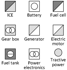 |
| PAH | Parallel hybrid passenger car with internal combustion engine and battery (addition of torque) | 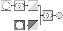 | |
| BEV | Electric passenger car with battery (battery-electric vehicle) | 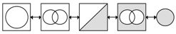 | |
| FCV | Fuel cell-electric vehicle with direct hydrogen operation and battery (fuel cell-electric vehicle) | 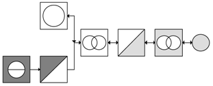 | |
| No. | Consumer | ICV | PAH | BEV | FCV |
|---|---|---|---|---|---|
| Powertrain | |||||
| 1 | Engine starter | 1900/2 s [24] | 1900/2 s | N.A. | N.A. |
| 2 | Control units | 200/C [24] | 200/C | 200/C | 200/C |
| 3 | Fuel supply | 135/C [24] | 135/C | N.A. | 135/C |
| 4 | Cooling fan | 500/D [24] | 500/D | 500/D | 500/D |
| 5 | Cooling pump | 50/C [29] | 100/C * | 50/D | 100/C |
| 6 | Power steering | All concepts: 500/D ** | |||
| Comfort | |||||
| 7 | PTC heating element | N.A. | Demand driven | ||
| 8 | Interior fan | All concepts: 120/D [28] | |||
| 9 | Seat heating | All concepts: 150/300 s [24] | |||
| 10 | Radio/navigation | All concepts: 150/C [29] *** | |||
| Safety | |||||
| 11 | Wipers f/r | All concepts: 160/D [24] | |||
| 12 | Window heater f/r | All concepts: 540/D [30] | |||
| Lighting | |||||
| 13 | Instruments | All concepts: 22/C [28] | |||
| 14 | Daytime running lights | All concepts: 12/C [26] | |||
| 15 | Low beam/tail lights | All concepts: 140/D Standard value, incl. license plate illumination | |||
| 16 | High beam | All concepts: 110/D Standard value | |||
| 17 | Brake lights | All concepts: 42/D Standard value | |||
| 18 | Turn signals | All concepts: 42/D Standard value | |||
| Parameter | Unit | A-Segment | C-Segment |
|---|---|---|---|
| Mass of the basic vehicle, | 800 | 1100 | |
| Reference area, | 1.8 | 2.1 | |
| Drag coefficient, | 0.32 | 0.32 |
| Parameter | Unit | A-Segment | C-Segment |
|---|---|---|---|
| Maximum speed | 160 (130) | 180 (160) | |
| Acceleration | 12 | 11 | |
| Maximum slope | 26.6 | 26.6 | |
| BEV range | 300 | 300 | |
| FCV range | 400 | 400 |
| Designation | Mean Velocity | Mechanical Energy |
|---|---|---|
| HYZEM | 68.4 | 56.9; −14.6 |
| HYZEM—urban | 22.3 | 51.2; −40.4 |
| HYZEM—rural | 47.5 | 51.4; −27.5 |
| HYZEM—highway | 91.9 | 58.7; −9.6 |
| Parameter | SUD | FRD |
|---|---|---|
| Temperature, amb/°C | 25 | 0 |
| Humidity, f/- | 40% | 80% |
| Solar radiation, Psol/(W m2) | 1000 | 0 |
| Initial cabin temperature, ϑ0,cab/°C | 22 | 22 |
| Function | ICV | PAH | BEV | FCV |
|---|---|---|---|---|
| Stop-start system | ■ | ■ | ■ | ■ |
| Regenerative braking | ☐ | ■ | ■ | ■ |
| Boost function | ☐ | ■ | ☐ | ■ |
| LPE/LPR/OPS | ☐/☐/■ | ■/■/■ | ☐/☐/■ | ■/■/■ |
| BE driving | n.a. | ■ | only mode | ■ |
| ICE driving | n.a. | ■ | n.a. | n.a. |
| Source | Type of Hybrid | Operational Strategy | Evaluation Function | Assessment Object |
|---|---|---|---|---|
| Altenthan [44] | Two-mode Full-Hybrid | Analytical heuristic | Minimize losses | BMW Two-mode hybrid SUV (gasoline engine) |
| Back [47] | PAH Mild-Hybrid | Predictive | Minimize consumption | Mercedes-Benz S-Class (gasoline engine) |
| Böckl [48] | PAH Mild-Hybrid | Adaptive predictive | Heuristic rules for controlling hybrid functions | VW Bora mild hybrid |
| Jörg [45] | PAH CVT-Hybrid | Predictive, heuristic (neural network) | Minimize power loss | TU Munich; CVT hybrid (Opel Vectra Caravan) |
| Kleimaier [43] | PAH CVT-Hybrid | Offline Online | Minimize power loss | TU Munich; autarkic hybrid (Opel Astra Caravan) |
| Körner [29] | SEH Full-Hybrid | Offline Online, FLC | Minimize consumption | Simulation and test rig for motor-generator units |
| Stiegeler [46] | PAH ASG | Predictive Analytical | Minimize consumption (cost function) | Theoretical and test rig for powertrain |
| Designation | Base Load 14 V Cons. | Additional 14 V Cons. | Heating & Cooling |
|---|---|---|---|
| BSL: “Baseload only“ | ■ | ☐ | ☐ |
| NHC: “No heating/cooling“ | ■ | ■ | ☐ |
| SUD: “Summer day“ | ■ | ■ | ■ (CL) |
| FRD: “Frost day“ | ■ | ■ | ■ (HE) |
| Concept|Car Segment | BSL | NHC | FRD | SUD |
|---|---|---|---|---|
| ICV–G/ICV–D|A-segment | ■ | ■ | ◪ | ☐ |
| ICV–G/ICV–D|C-segment | ■ | ■ | ◪ | ☐ |
| PAH–G/PAH–D|A-segment | ■ | ■ | ■ | ■ |
| PAH–G/PAH–D|C-segment | ■ | ■ | ■ | ■ |
| BEV|A-segment | ■ | ■ | ■ | ■ |
| BEV|C-segment | ■ | ■ | ■ | ■ |
| FCV|A-segment | ■ | ■ | ■ | ■ |
| FCV|C-segment | ■ | ■ | ■ | ■ |
| Parameter | Dimension | “Standard” | “Advanced” |
|---|---|---|---|
| Air drag coefficient | 0.32 | 0.27 [50] | |
| Rolling resistance | Improvement after [51] | ||
| Glider mass, A-|C-segment | 800|1000 | 720|900 | |
| Efficiency of internal combustion engine | Improved performance | ||
| Efficiency of electric machine | Improved performance | ||
| Efficiency of fuel cell | Improved u-i performance | ||
| Specific power of fuel cell system | 0.400 [52] | 0.650 [52] | |
| Specific energy of H2 tank | 1800 | 2160 | |
| Specific energy of battery | 100 | 150 | |
| Heating & cooling power | Reduced by 20% | ||
© 2018 by the authors. Licensee MDPI, Basel, Switzerland. This article is an open access article distributed under the terms and conditions of the Creative Commons Attribution (CC BY) license (http://creativecommons.org/licenses/by/4.0/).
Share and Cite
Grube, T.; Stolten, D. The Impact of Drive Cycles and Auxiliary Power on Passenger Car Fuel Economy. Energies 2018, 11, 1010. https://doi.org/10.3390/en11041010
Grube T, Stolten D. The Impact of Drive Cycles and Auxiliary Power on Passenger Car Fuel Economy. Energies. 2018; 11(4):1010. https://doi.org/10.3390/en11041010
Chicago/Turabian StyleGrube, Thomas, and Detlef Stolten. 2018. "The Impact of Drive Cycles and Auxiliary Power on Passenger Car Fuel Economy" Energies 11, no. 4: 1010. https://doi.org/10.3390/en11041010
APA StyleGrube, T., & Stolten, D. (2018). The Impact of Drive Cycles and Auxiliary Power on Passenger Car Fuel Economy. Energies, 11(4), 1010. https://doi.org/10.3390/en11041010