An Artificially Intelligent Technique to Generate Synthetic Geomechanical Well Logs for the Bakken Formation

Abstract

Artificially intelligent and predictive modelling of geomechanical properties is performed by creating supervised machine learning data models utilizing artificial neural networks (ANN) and will predict geomechanical properties from basic and commonly used conventional well logs such as gamma ray, and bulk density. The predictive models were created by following the approach on a large volume of data acquired from 112 wells containing the Bakken Formation in North Dakota. The studied wells cover a large surface area of the formation containing the five main producing counties in North Dakota: Burke, Mountrail, McKenzie, Dunn, and Williams. Thus, with a large surface area being analyzed in this research, there is confidence with a high degree of certainty that an extensive representation of the Bakken Formation is modelled, by training neural networks to work on varying properties from the different counties containing the Bakken Formation in North Dakota. Shear wave velocity of 112 wells is also analyzed by regression methods and neural networks, and a new correlation is proposed for the Bakken Formation. The final goal of the research is to achieve supervised artificial neural network models that predict geomechanical properties of future wells with an accuracy of at least 90% for the Upper and Middle Bakken Formation. Thus, obtaining these logs by generating it from statistical and artificially intelligent methods shows a potential for significant improvements in performance, efficiency, and profitability for oil and gas operators.

1. Introduction

North Dakota has been an oil producing state for over 60 years, but only during the past few years has the Bakken oil boom made it to one of the largest hydrocarbon-producing states in the US. As of 2017, estimates of about 4.4 to 11.4 billion barrels of undiscovered yet technically recoverable oil, and 6.7 trillion cubic feet of associated natural gas and 0.53 billion barrels of natural gas has made North Dakota’s Bakken draw a lot of attention. Emerging infrastructure developments along with innovative technologies have been poured down upon the Bakken Formation to effectively extract from the unconventional reservoir and transform the prospects for U.S. field production in the coming years. To efficiently produce from unconventional reservoirs, it is imperative to determine and understand the geomechanical properties of the formation. Successful wellbore stability, drilling design, and hydraulic fracturing techniques are some of the key results of fully understanding the geomechanical properties of the formation. However, with the high cost associated with obtaining geomechanical well logs, the usage of these logs can be limited, and are not widely used. Thus, this study will show an alternate and cost-efficient technique, yet accurate estimation of geomechanical properties for current and future wells by using artificial intelligence and predictive modelling.

Additionally, shear wave velocity will also be analyzed using regression technique [1,2,3,4], and a new correlation will be proposed for the Upper and Middle Bakken Formation. In comparison to regression techniques, shear wave velocity will also be predicted using artificial neural networks (ANN). This will be done by creating supervised machine learning data models utilizing ANN that will predict shear wave velocity, and geomechanical properties from commonly used conventional well logs such as gamma ray, and bulk density. North Dakota will be the focus of this study, and the application of this study will be developed from large volumes of data attained from 112 wells of the Bakken Formation in North Dakota.

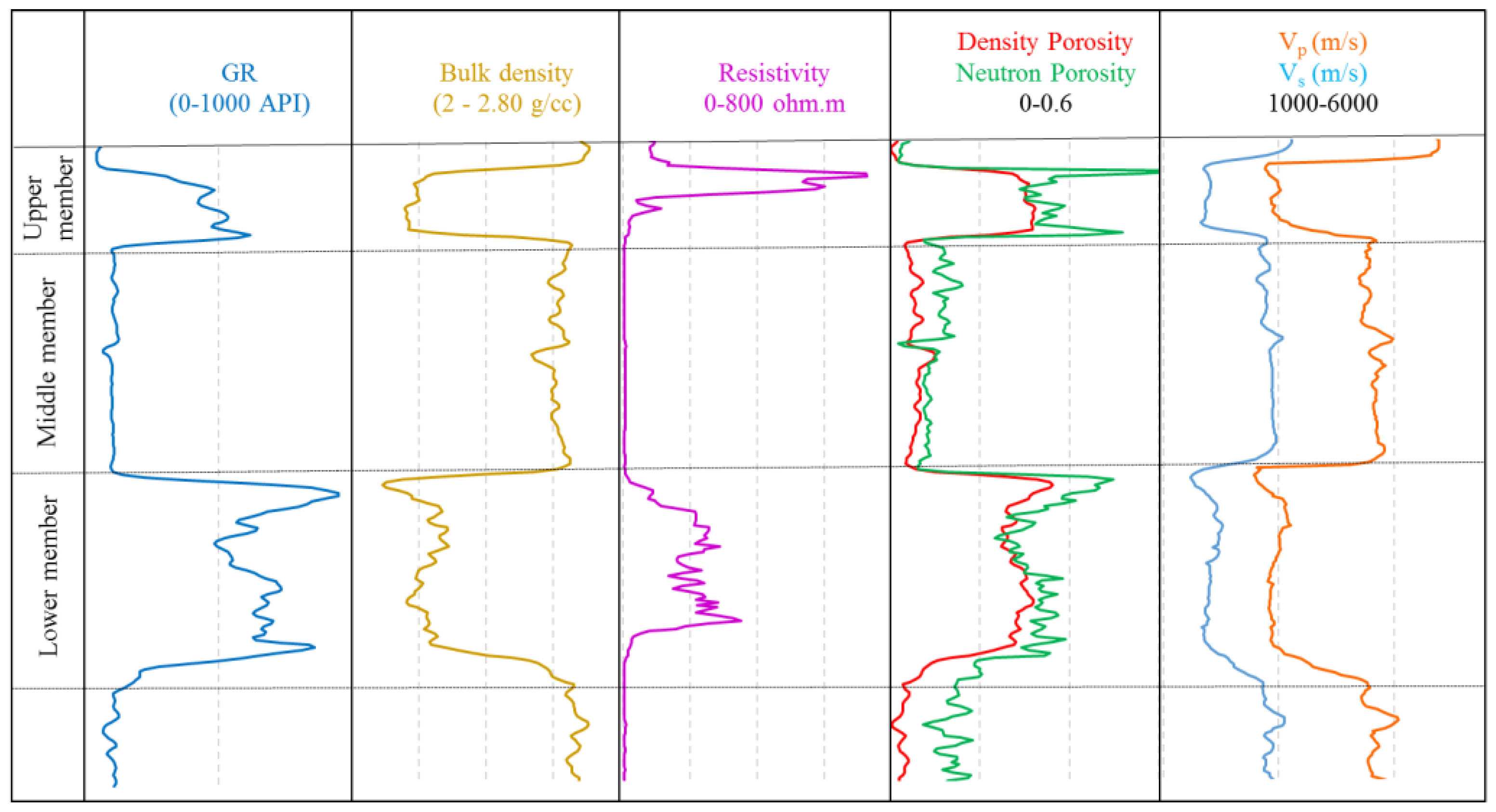
The Bakken formation is located at depths between 8000 feet to 11,000 feet and has a total thickness of approximately 140 feet [5]. The upper and lower members of the Bakken Formation are organic rich shales and are very uniform throughout their extents. They serve as source rocks for oil and natural gas, and as seals for the Three Forks Formation, and the Middle Bakken Formation. The Upper member has a thickness ranging from 20 feet to 58 feet, whereas the Lower member has a thickness between 45 feet to 56 feet [6,7], and are easily recognizable in wireline logs because of the unusually high gamma ray readings of over 400 API, low bulk density, and low compressional and shear wave velocities, all associated with high organic content (Figure 1). The middle member, sandwiched between the upper and lower members, is composed of dolomitic siltstone, sandstone, laminated calcareous siltstone, bioturbated calcareous siltstone, and fossiliferous calcareous siltstone; with a thickness ranging from 30 feet to 70 feet (Figure 1), and is the main producing member in the formation [8]. Since the middle member’s lithology is highly variable and consists of five distinct lithofacies, hence there is high heterogeneity present in this member [9]. All lithologies within the middle member have low porosity and permeability with values ranging from 2% to 10% and from 0.000001 to 2 mD, respectively [10].

Artificial Neural Networks (ANN) can be very good predictors in determining the relationship between the inputs and the outputs which at times seem pattern-less. Previous studies show that neural networks have been used to predict different reservoir properties such as porosity, permeability, and fluid saturation to reduce the cost of utilizing expensive processes to acquire those properties [12,13,14,15,16,17]. Neural networks were also used to generate synthetic well logs and perform reservoir modelling and analysis of formation characteristics [18,19]. With the recent advancements in shale recovery and hydraulic fracturing, machine learning was successfully used to identify sweet spots in shale-gas reservoirs [20]. Artificial neural networks were also used to generate synthetic geomechanical well logs from conventional well logs for Marcellus Shale, showing its use in minimizing cost in acquiring geomechanical logs [21,22]. All the previous studies and work done above have one goal in mind; to utilize statistical and artificially intelligent methods to improve the understanding of formation characteristics with ease, and efficiently enhance the productivity from the reservoir. Similarly, this study also follows a similar goal in utilizing an alternate and efficient technique to help operators obtain a better understanding of the formation with ease, by processing large volumes of data from 112 wells, and transforming it into high value information that could ultimately help operators produce more from current and future wells. The strategy proposed is to minimize input logs to just basic and commonly used well logs that predict shear wave velocity and geomechanical properties with high accuracy, to minimize cost and algorithm processing time without compromising the predictive capability and reliability of the model [23].

One hundred and twelve wells from five of the main producing counties in North Dakota containing the Upper and Middle Bakken Formation are taken into consideration. First, a study will be conducted to predict shear wave velocity by linear and non-linear methods. Shear wave velocity is crucial in making reliable calculations, especially to calculate the missing dynamic geomechanical properties of the Upper and Middle Bakken wells. Once the missing values of dynamic geomechanical properties are calculated, and the database is complete with all the required parameters, supervised machine learning data-driven models will then be developed to predict geomechanical properties for future wells. The results and benefits of the developed data models will then be demonstrated and tested on 5 additional validation wells of the Bakken Formation to confidently assure its efficacy and working capabilities on future wells of North Dakota.

2. Methodology

Artificial neural networks (ANN) are computational models based on a collection of neural units modelling the problem-solving skills of the brain. Their neural units are compared specifically to the neurons within the brain. ANN mimics the brain’s pattern recognition capabilities to solve complex non-linear functions [24]. A multilayer perceptron type of ANN model is used extensively in this research. The multilayer perceptron is a fully connected multilayer feed forward supervised learning network with symmetric hyperbolic tangent activation functions, trained by the back-propagation algorithm [25]. 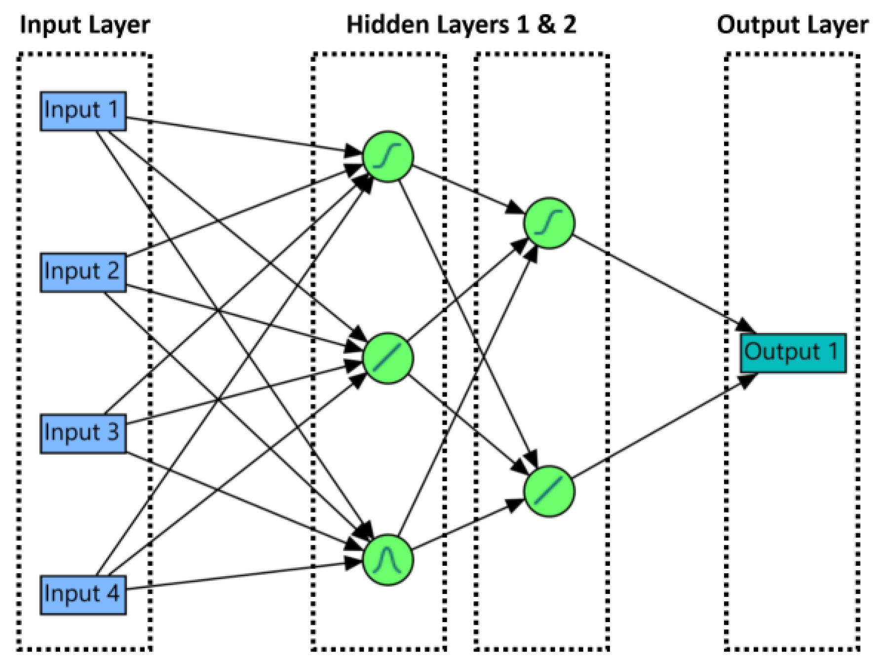Figure 2 shows an illustration of the ANN model being used, and the number of nodes carrying the activation function within the hidden layers performed in this research will vary for each ANN model obtained to produce the most efficient results as outputs. The various activation functions used within the nodes in this research are [26]:

• Hyperbolic Tangent Function (Sigmoid Function)—Transformation of values to be between −1 and 1 (Equation (1)). It is the centered and scaled version of the logistic function.

  $$\frac{e^{2x}-1}{e^{2x}+1}$$

  (1)

  where x is the linear combination of the input variables.
• Linear Function (Identity Function)—The linear combination of the input variables is not transformed in this function. This activation function is mostly used with one of the non-linear activation functions to reduce the dimensionality of the input variables first, and then have a nonlinear model for the output variables.
• Gaussian Function (Normal Distribution)—This activation function is used when the inputs follow a normal distribution (Equation (2)).

  $$e^{-x^2}$$

  (2)

  where x is a linear combination of the input variables.

A total of 14 ANN models were developed to successfully complete the research. All the models follow the same principle, and are multilayer models trained using back propagation algorithm, where 70% of the data was used for training, and 30% of the data was used for verification. This is done by randomly dividing the original combined dataset into the training and validation sets and using Monte-Carlo cross-validation with a randomly selected proportion of 30% for verification [23]. However, the inferring of the number of nodes carrying the activation functions within the hidden layers performed in this research was obtained by trial and error technique and will vary for each of the 14 ANN models obtained to produce the most optimal structure and ultimately provide efficient results as outputs.

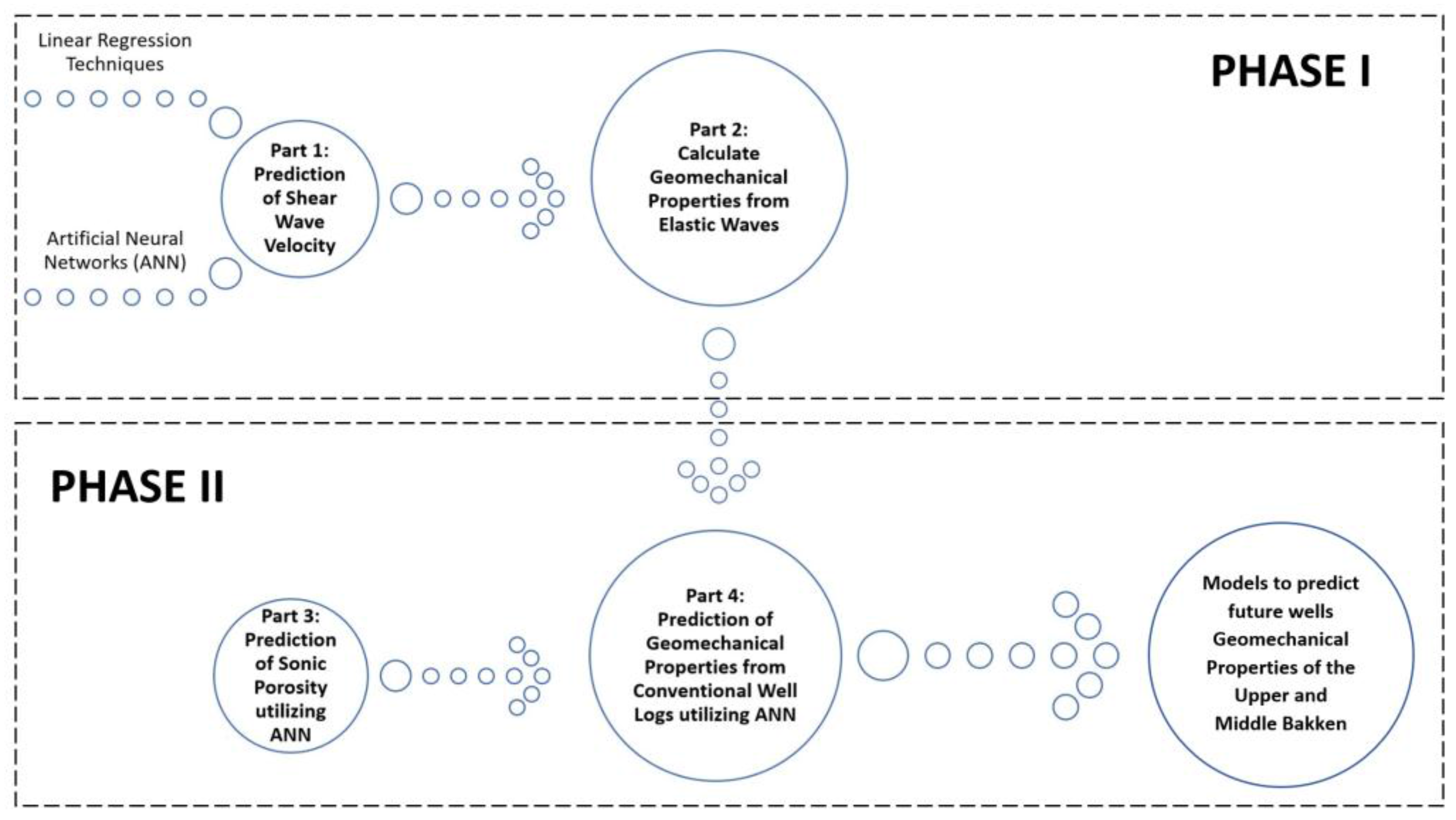
The study is broken down into two phases as shown in Figure 3.

2.1. PHASE I: Calculation of Geomechanical Properties of the Upper and Middle Bakken Formation from Elastic Waves

In this phase, geomechanical properties of the Upper and Middle Bakken Formation are calculated dynamically from compressional wave velocity and shear wave velocity. Since the geomechanical properties of wells were not provided in the logs for 63 wells, they have been calculated dynamically from elastic waves, i.e., shear wave and compressional wave. Thus, the purpose and goal of phase I is to fill up the missing values of geomechanical properties of all the wells in the database, without which phase II cannot be performed. Phase I has been broken down into two parts. Part 1 will predict shear wave velocity for missing wells. Once the database for shear wave velocity is complete, part 2 will be to calculate geomechanical properties dynamically from elastic waves.

Table 1. Data available for the prediction of Shear Wave Velocity.

Group	Number of Wells	Conventional Well Logs				Geomechanical Well Logs
		Gamma Ray	Bulk Density	Compressional Wave Velocity	Shear Wave Velocity
Phase I	49	Yes	Yes	Yes	Yes	Yes
	63	Yes	Yes	Yes	No	No

shows the available data to proceed with this part.

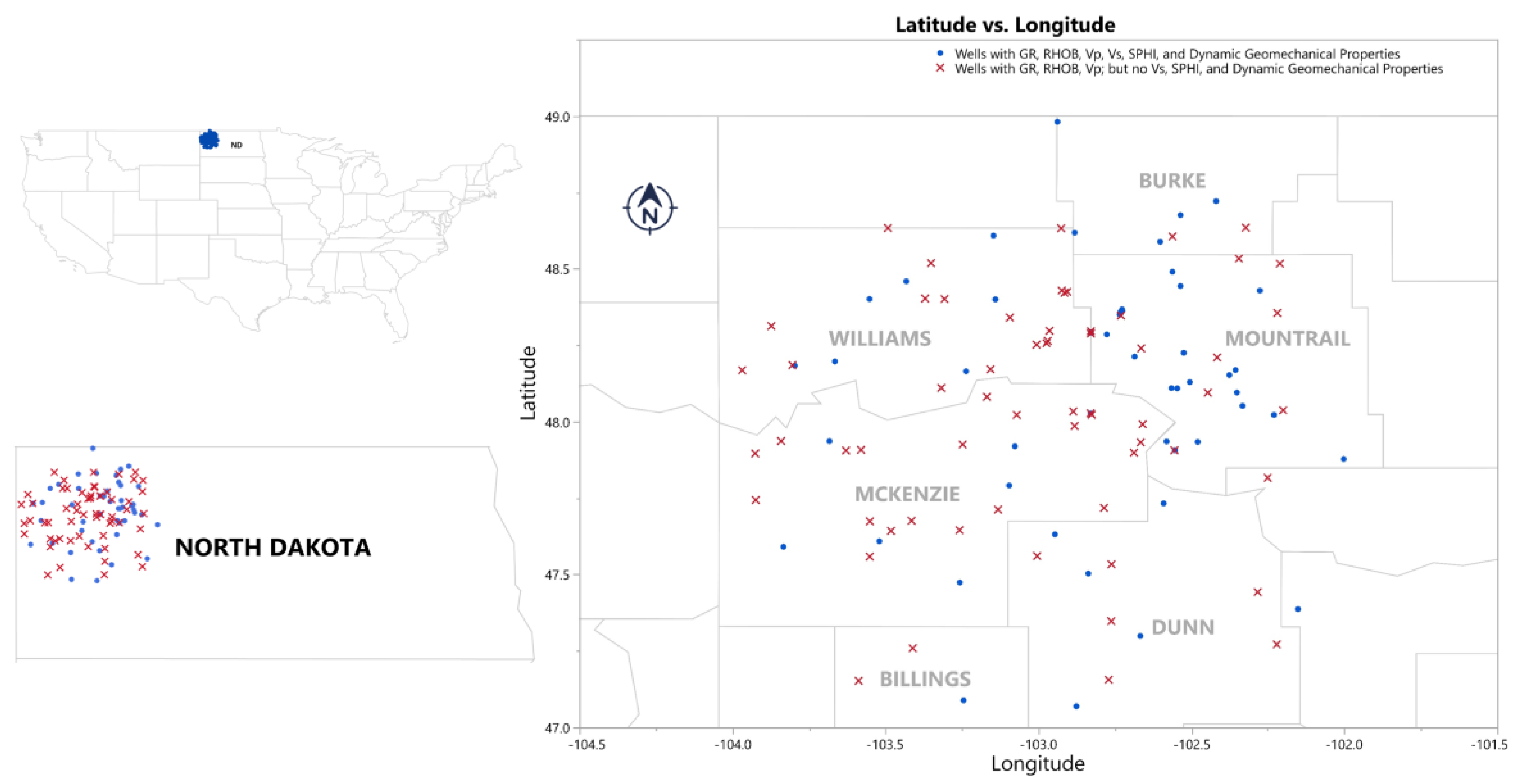
Figure 4 shows the Bakken area of North Dakota, and the distribution of 112 wells with respect to gamma ray, bulk density, compressional and shear wave velocity, sonic porosity, and geomechanical properties. Since 63 wells do not contain information on shear wave velocity, the dynamic geomechanical properties for 63 wells are also incomplete. Hence it is essential to predict shear wave velocity for 63 wells to calculate the geomechanical properties for 63 wells. By this process, the geomechanical properties database will be complete, and we can proceed to input into phase II.

2.1.1. Part 1: Prediction of Shear Wave Velocity

To have consistent information of all wells, it is necessary to predict and generate data for the missing information. All 112 wells have compressional wave velocity (derived from compressional wave slowness), but only 49 wells have information on shear wave velocity (derived from shear wave slowness). Thus, to calculate the geomechanical properties dynamically from elastic waves, it is necessary to fill up the missing values of shear wave velocity for 63 wells.

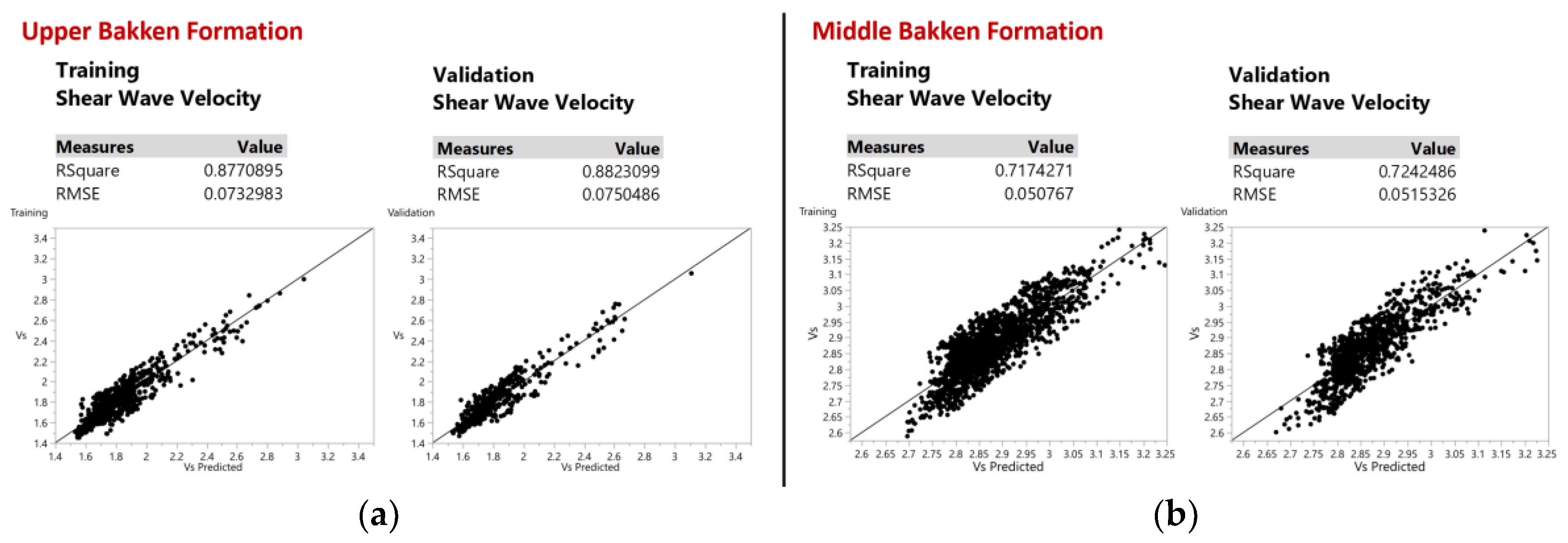
Step A: Prediction of Shear Wave Velocity from Compressional Wave Velocity utilizing Linear Regression Techniques.

In this step, a linear approach is used, to create a correlation between shear wave velocity (V_s) and compressional wave velocity (V_p), and then the shear wave velocity is determined for the missing wells. Figure 4 shows the distribution of all wells with respect to information regarding compressional wave velocity and shear wave velocity. A Monte-Carlo cross-validation technique was also performed to show the predictive capability of the model, where 70% was used for training and 30% was used for verification, and a model is developed which predicts the shear wave velocity (V_s) for 63 wells. Figure 5 shows the visualization of the training set and validation set for predicting shear wave velocity with an accuracy of 88% and 72% for both the Upper and Middle Bakken Formation respectively.

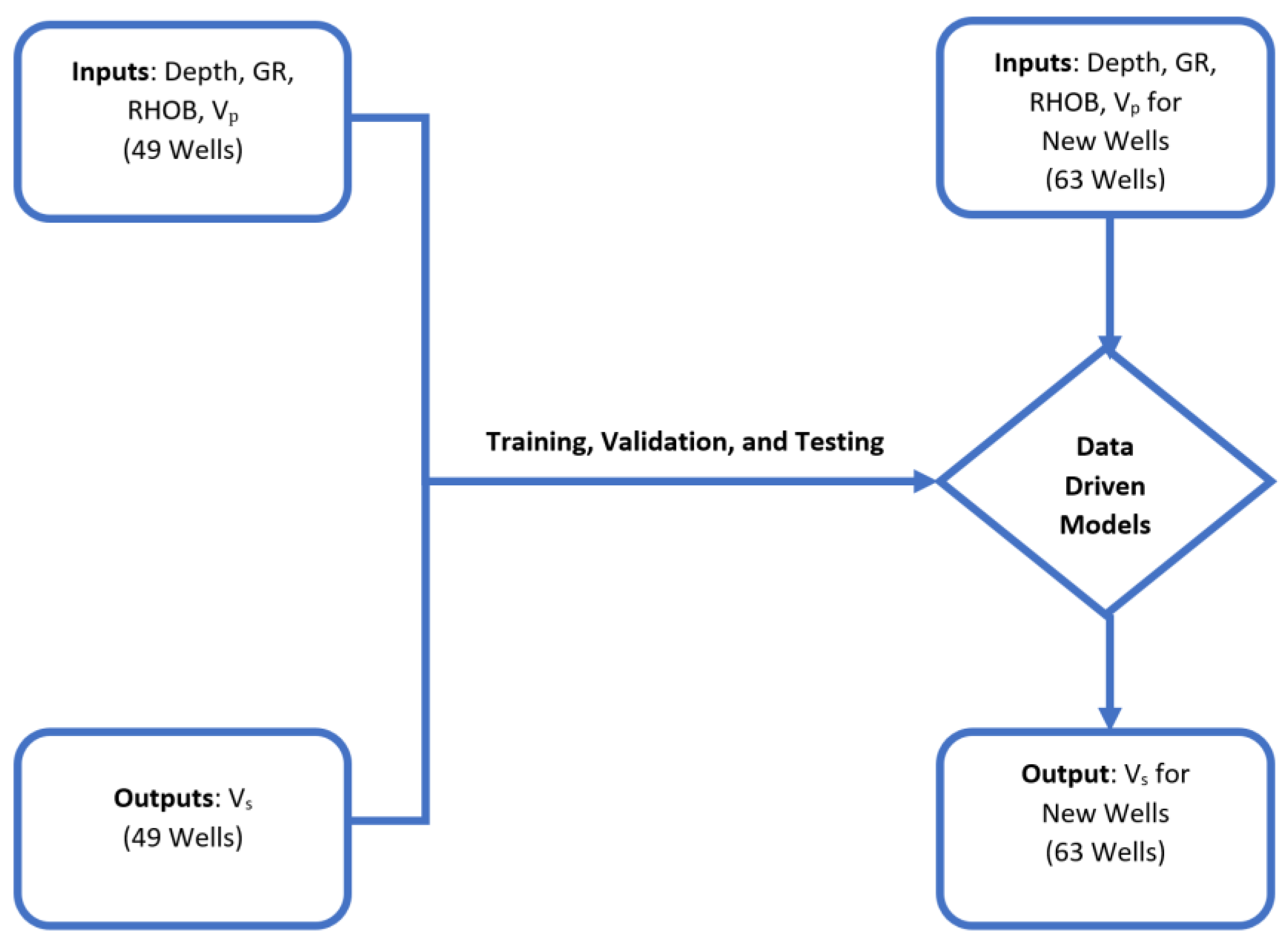
Step B: Prediction of Shear Wave Velocity from Conventional Well Logs utilizing ANN

An ANN model was developed by using conventional well logs as the input and shear wave velocity as the output. Initially, the conventional well logs used were depth, gamma ray (GR), and bulk density (RHOB). The results obtained for predicted shear wave velocity were unsatisfactory, resulting in a very low R², indicating that a pattern was not fully recognized, and an additional input was necessary to improve the reliability of the model. Thus, compressional wave velocity was added as an additional input along with other conventional well logs.

Figure 4 shows the distribution of wells with respect to information regarding depth, gamma ray (GR), bulk density (RHOB), compressional wave velocity (V_p), and shear wave velocity (V_s). Figure 6 shows the process flow for the creation of the neural network model using depth, gamma ray (GR), bulk density (RHOB) and compressional wave velocity (V_p) for 49 wells and the output of shear wave velocity (V_s) for 49 wells. 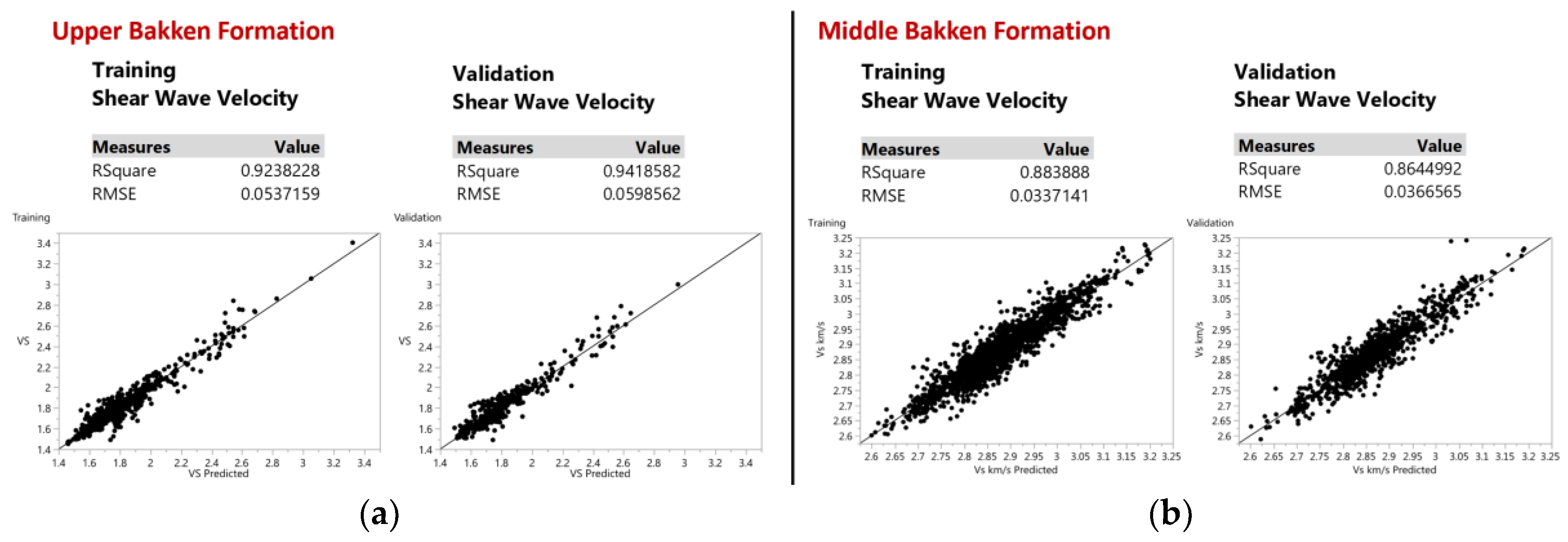The ANN model is trained and validated, where 70% was used for training and 30% was used for verification using Monte-Carlo cross-validation technique, and a model is developed which predicts the shear wave velocity (V_s) for 63 wells. Figure 7 shows the visualization of the training set and validation set for predicting shear wave velocity with an accuracy of 94% and 86% for both the Upper and Middle Bakken Formation respectively.

Step C: Comparison of results of different models to predict Shear Wave Velocity.

In this step, the linear regression and ANN models used to achieve shear wave velocity for the missing wells are compared. The model resulting in better prediction and accuracy of shear wave velocity as compared to the actual shear wave velocity is selected as the model to estimate the shear wave velocity for the remaining 63 wells. In this study, the ANN model predicts shear wave velocity with higher accuracy of 94% and 86% as compared to a linear regression technique with an accuracy of 88% and 72% for the Upper and Middle Bakken Formation respectively. Both models have significantly high accuracy, however in this research, shear wave velocity will be predicted from ANN for 63 wells to proceed with the next part of the research. A detailed explanation of the comparison is seen below at the results and discussions Section 3.1.3.

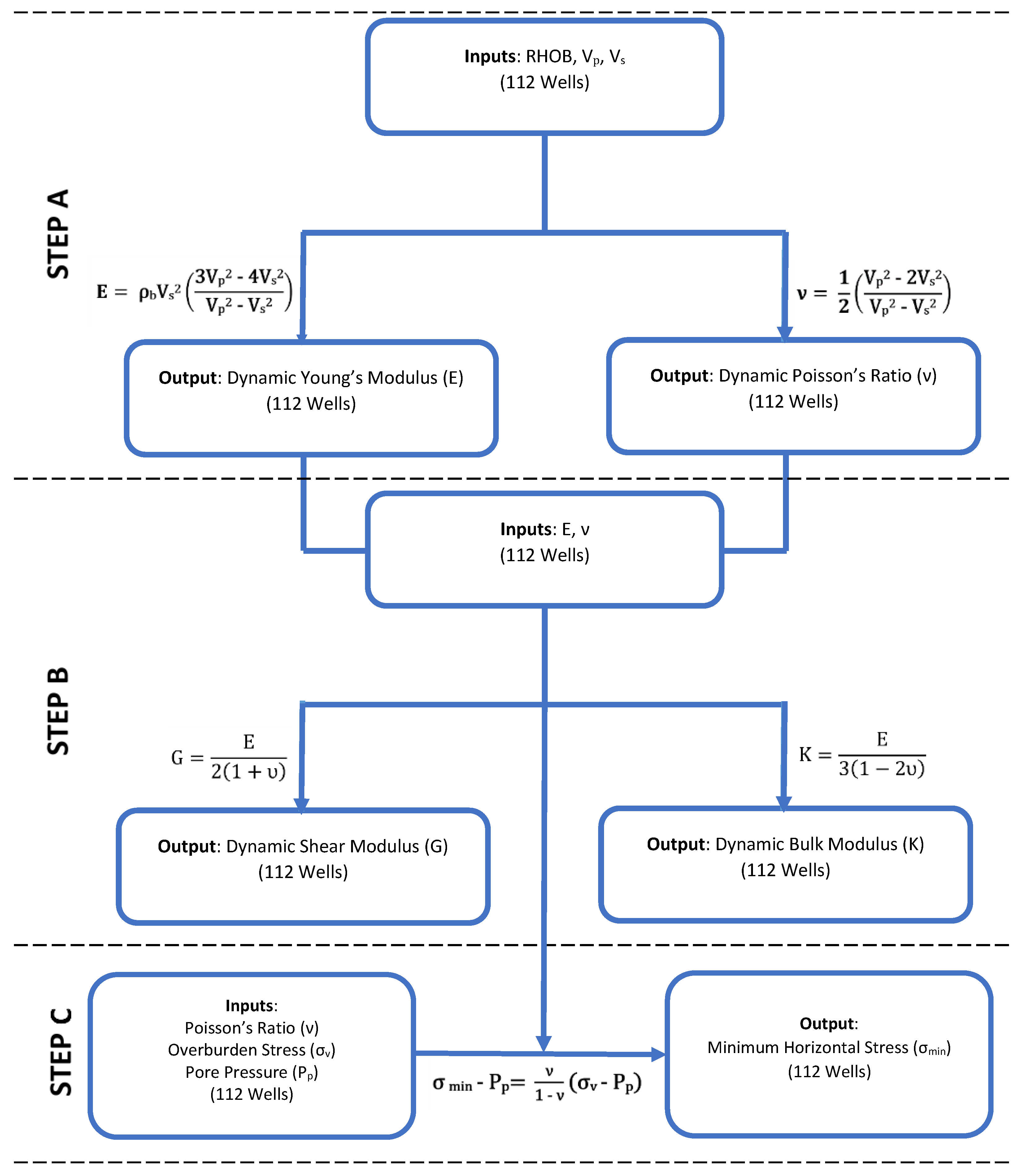
2.1.2. Part 2: Calculate Geomechanical Properties Dynamically from Elastic Waves.

After having the information for both compressional wave velocity (V_p) and shear wave velocity (V_s) for all 112 wells, the geomechanical properties can now be dynamically calculated from elastic waves. The properties of the Upper and Middle Bakken Formation are assumed to be isotropic in this research, and thus there are two independent elastic constants [27]. In other words, two elastic constants are enough to derive the other elastic constants. Young’s Modulus and Poisson’s Ratio were first calculated from elastic waves, and then are used to calculate Shear Modulus, Bulk Modulus and Minimum Horizontal Stress. Figure 8 shows the flowchart process to calculate the geomechanical properties from elastic waves.

Ultimately, the Minimum Horizontal Stress (σ_min) for 112 wells is calculated using Eaton’s Equation [28]. Poisson’s Ratio (ν) calculated from Step A for 112 wells is used as the input along with Overburden Stress (σ_ν) imposed on the rocks from the weight of the overlying rocks, and Pore Pressure (P_p) from the fluids held within the rocks, and the generation of hydrocarbons. The Upper Bakken Shale is moderately over pressurized and is assumed to have a pore pressure of 0.65 psi/ft, and 0.55 psi/ft for the Middle Bakken Formation as the pore pressure decreases significantly away from the shales [29]. The overburden stress has been calculated and approximated to be 1.07 psi/ft for this research by using Eaton’s equation. However, since minimum horizontal stress is a key factor in understanding the directions to fracture the formation, hence we have proceeded with only predicting the minimum horizontal stress, and thus suffers the calculation and prediction of the maximum horizontal stress.

2.2. PHASE II: Geomechanical Properties of the Upper and Middle Bakken Formation Available after Utilizing Data Mining Techniques and ANN

After the completion of phase I, the geomechanical properties of the Upper and Middle Bakken Formation have been calculated from elastic waves and the missing information of geomechanical properties have been filled up in the database. This leads to the implementation of phase II, where the geomechanical properties calculated from phase I are predicted using conventional well logs, as to obtain a data-driven model that can ultimately predict geomechanical properties of future wells drilled in the Bakken Formation of North Dakota.

For the successful completion of Phase II, it has been broken down into 2 parts. Part 3 will predict sonic porosity for missing wells. Once the database for sonic porosity is complete, part 4 will be to predict geomechanical properties from conventional well logs utilizing ANN. The following parts are mentioned in detail below:

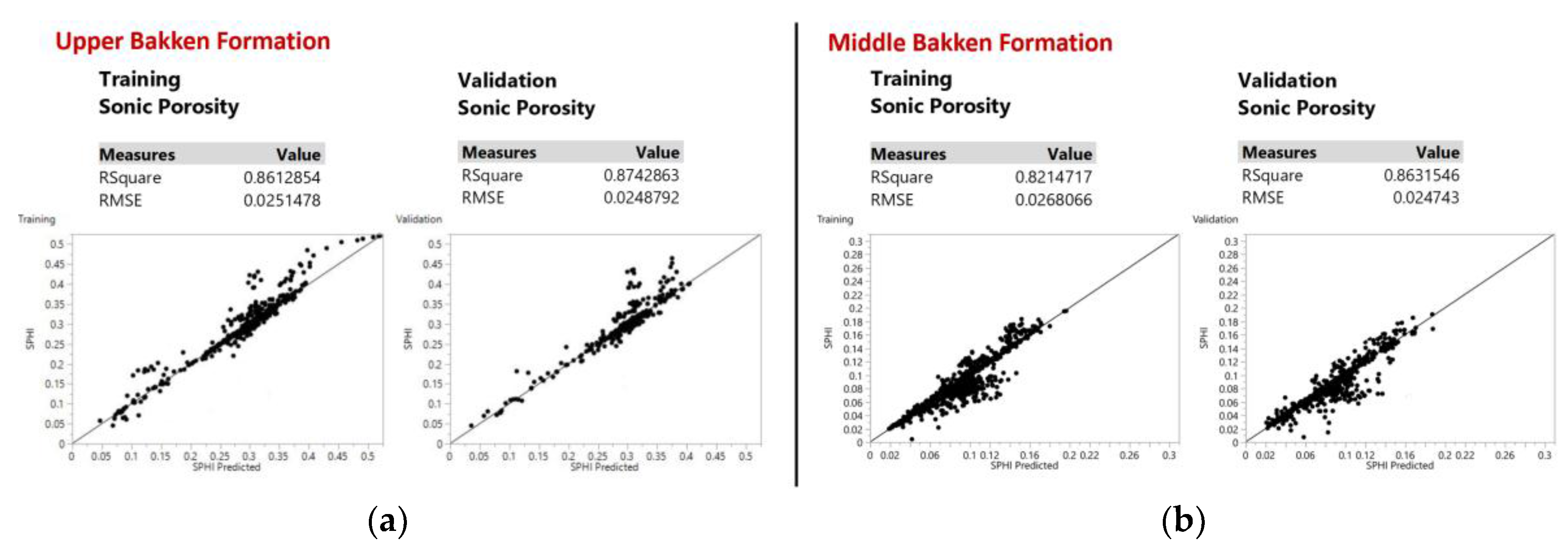
2.2.1. Part 3: Prediction of Sonic Porosity from Conventional Well Logs Utilizing ANN.

In this part, sonic porosity (SPHI) is determined from conventional well logs to fill in the missing sonic porosity values.

Table 2. Data available for the prediction of Sonic Porosity.

Group	Number of Wells	Conventional Well Logs			Geomechanical Well Logs
		Gamma Ray	Bulk Density	Sonic Porosity
Phase II	49	Yes	Yes	Yes	Yes
	63	Yes	Yes	No	Yes

shows the available data to proceed with this part. An ANN model was developed by using conventional well logs as the independent input variable and sonic porosity as the output dependent variable.

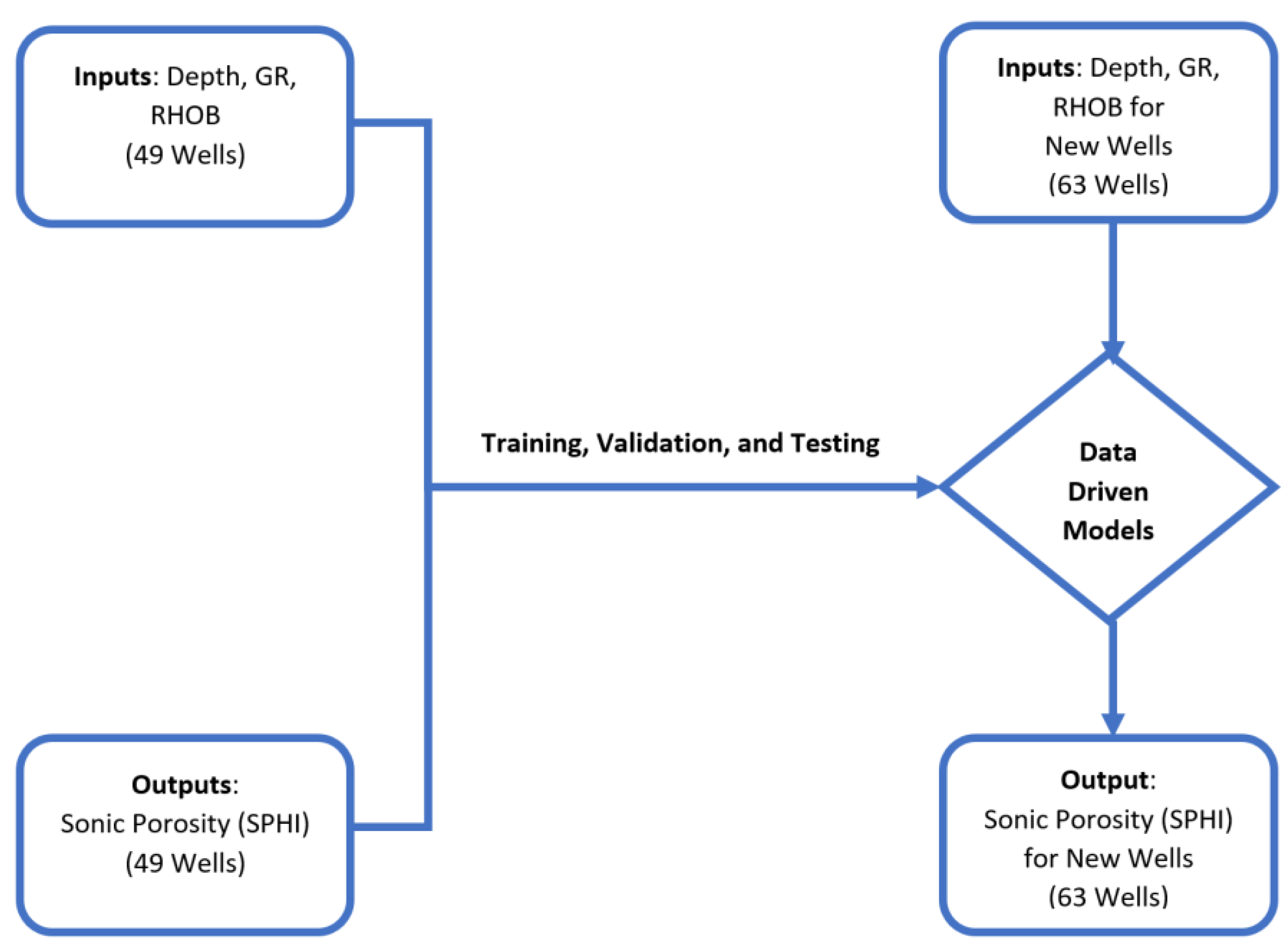
From Figure 4, the distribution of wells with respect to information regarding depth, gamma ray (GR), bulk density (RHOB), and sonic porosity (SPHI) were seen. ANN is used to create a pattern between sonic porosity (SPHI) and conventional well logs. Figure 9 shows the process flow of the creation of the neural network model using depth, gamma ray (GR), and bulk density (RHOB) for 49 wells and the output of sonic porosity (SPHI) for 49 wells. At the end of part 3, sonic porosity (SPHI) will be present for all 112 wells in the asset.

The ANN model is trained and validated, where 70% was used for training and 30% was used for verification using Monte-Carlo cross-validation technique, and a model is developed which predicts the Sonic Porosity (SPHI) for 63 wells. Figure 10 shows the visualization of the training set and validation set for predicting sonic porosity with an accuracy of 87% and 86% for both the Upper and Middle Bakken Formation respectively.

2.2.2. Part 4: Prediction of Geomechanical Properties from Conventional Well Logs Utilizing ANN

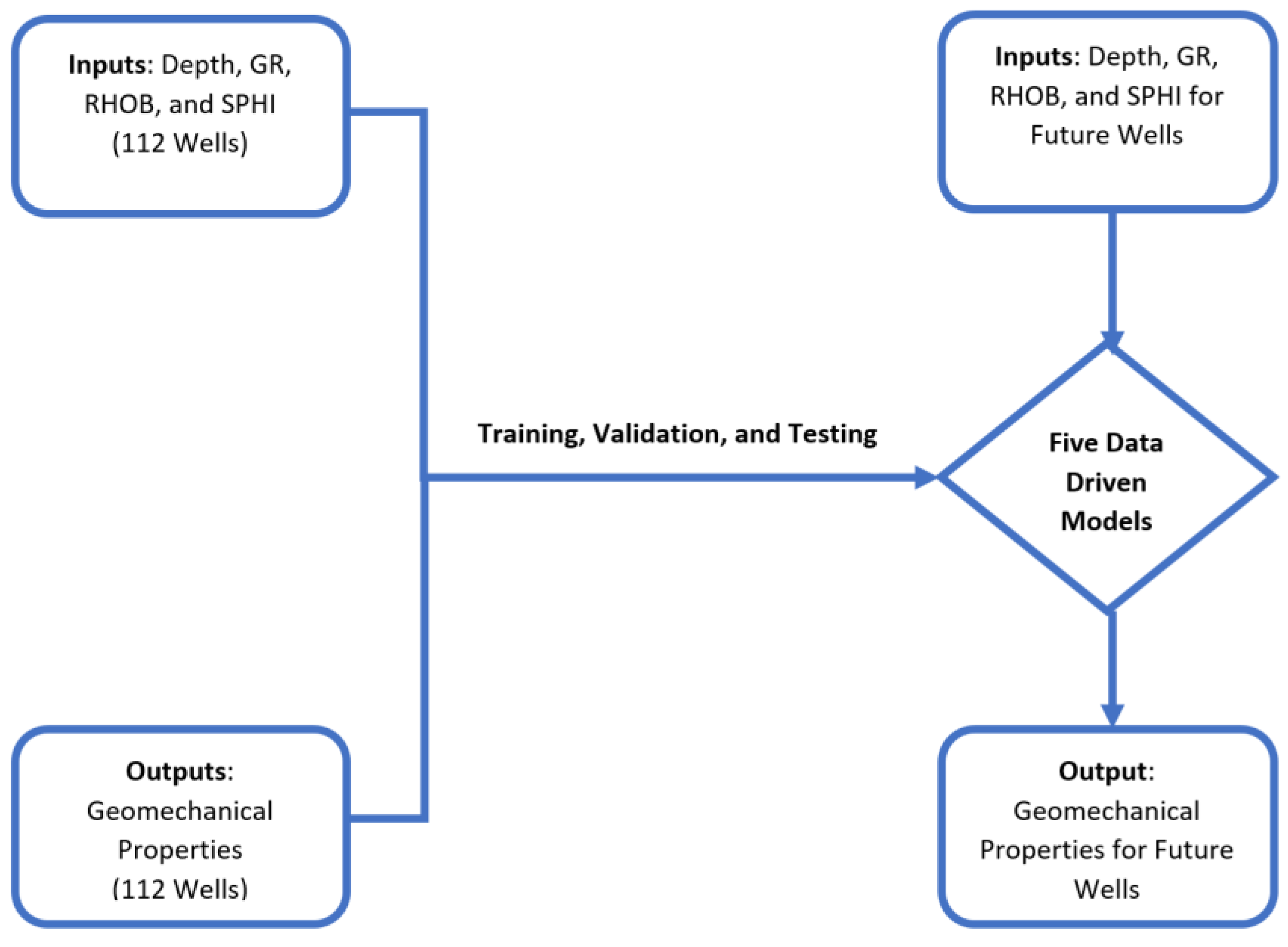
At this stage, all 112 wells in the asset have information on conventional well logs as the input independent variables including sonic porosity (SPHI) as the additional input, and geomechanical properties as the output dependent variables. In this part, a data-driven model is generated that will predict geomechanical properties just from conventional well logs for future wells, and this was done by using conventional well logs as the independent input variables and geomechanical properties as the output dependent variables. Five ANN models will be achieved for each formation, with each model generating a single geomechanical property for the Upper and Middle Bakken Formation. For each neural network model, the geomechanical property output generated in the previous model will be used as an input along with the conventional well logs to predict the next geomechanical property. This process continues until all five geomechanical property data-driven models are obtained.

In Figure 11, the neural network uses depth, gamma ray (GR), bulk density (RHOB), and sonic porosity (SPHI) as the input, and the output of five geomechanical properties for 112 wells. At the end of part 4, five data-driven models are generated that will predict geomechanical properties just from conventional well logs for future wells drilled in the Upper and Middle Bakken Formation. The ANN model is trained and validated, where 70% was used for training and 30% was used for verification using Monte-Carlo cross-validation technique. Overall, the 10 models obtained from neural networks predicting geomechanical properties for the Upper and Middle Bakken Formation achieved R² over 90%.

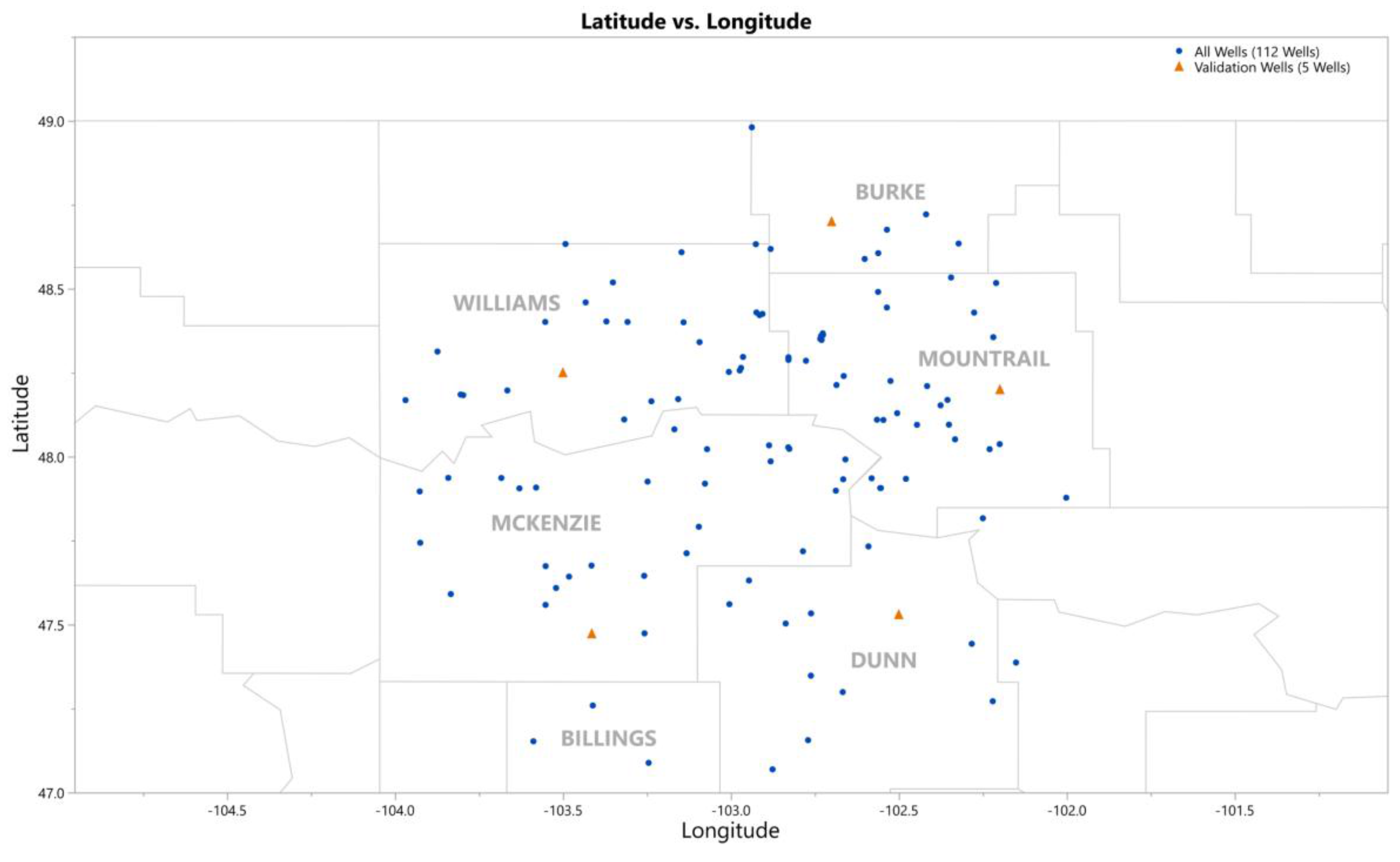
In addition to the 30% validation performed above, the efficacy of the 5 models achieved above is tested again and can be proven on 5 randomly selected test wells, one from each of the five major counties containing the Upper and Middle Bakken Formation as seen in Figure 12. It is also important to note that the actual geomechanical properties from the well logs obtained by the operators from the 5 randomly chosen test wells containing the Upper Bakken Shale and Middle Bakken Formation were not used in the dataset to train the ANN models achieved in phase II. In other words, the ANN models achieved in phase II will use input parameters of depth, gamma ray, and bulk density from each of the 5 test wells separately and generate the output of predicted geomechanical properties for each of the 5 wells. The predicted geomechanical property output will then be compared to the actual geomechanical logs of the 5 test wells obtained by the operators. This approach will prove the efficacy of the ANN models achieved in phase II, showing that the model can be used to predict geomechanical properties of future wells making it very cost effective for operators operating out of North Dakota for the Upper and Middle Bakken Formation.

3. Results and Discussion

It is important to note that although phase I is used to calculate the geomechanical properties of the Upper and Middle Bakken Formation which is used as a prequel to phase II, phase I is not required and will not be used in the algorithm to predict the geomechanical properties of future wells from conventional well logs. In a simpler understanding of this research, phase I was an additional section used only to calculate the geomechanical properties dynamically from elastic waves, to fill up the database with the missing values of geomechanical properties. Since phase I is an additional section in this research, a relationship between shear wave velocity and compressional wave velocity was also established using linear and non-linear techniques as additional information to this research. In all aspects, the main goal of this research is phase II, which is to successfully achieve data-driven models that use basic and commonly used well logs in the industry such as depth, gamma ray, and bulk density to predict sonic porosity, which in turn is used as the input with the other input parameters to predict the geomechanical properties of future wells of the Upper and Middle Bakken Formation, thus making it very cost effective for oil and gas operators.

A total of 14 ANN models were achieved to predict shear wave velocity, sonic porosity, and 5 geomechanical properties for the Upper and Middle Bakken Formation each. In this research, the number of nodes carrying the activation functions of sigmoid, linear, and Gaussian within the hidden layers vary for each ANN model, and an optimal structure was achieved through trial and error technique for each model. For each model, 2 hidden layers were used, but the number of nodes carrying the activation functions varied for each ANN model based on their output property. This was done to produce highly accurate results as outputs, and thus a definite structure of the model cannot be elaborated in this research. Overall, the neural network models are trained using back propagation technique with multilayer perceptrons, which helps in faster learning making it possible to find a pattern between variables that had previously been deemed pattern-less and unpredictable [25,30]. The main advantage of a neural network model is that it can efficiently model different response surfaces and can be approximated to any accuracy. Neural networks are very flexible models but tend to overfit data. When that happens, the model predicts the fitted data very well, but predicts future observations poorly. To mitigate overfitting, neural network uses a validation technique that uses part of the dataset in the training set to estimate the model parameters and using the other part in the validation set to validate the predictive ability of the model. The partitioning of the dataset into training and validation set is arbitrary and can vary depending on the situation and the developer’s choice. In this research, 70% of the data was used for training and 30% of the data was used for verification, which is an ideal choice for this research, providing sufficient amount of data for training the model and finally verifying the model. This is done by randomly dividing the original combined dataset into the training and validation sets by using a Monte-Carlo holdback validation with a proportion of 30% for verification. A weight decay penalty is also applied on model parameters by penalizing large weights on their squared value or absolute value. This is done to prevent the overfitting and overtraining effect. Finally, an independent test set is used to assess the model’s predictive ability independently.

The continuous input variables in neural networks are transformed to near normality by using Johnson’s Distribution [31], to mitigate the negative effects of outliers or heavily skewed distributions. Boosting is also performed on neural networks at a slow learning rate of 0.1 making the model give better predictions. If the updated model gives better prediction than the previous model, it replaces the previous model achieved. This is done by building a large additive neural network model by fitting a sequence of smaller models. Each of the smaller models is fit on the scaled residuals of the previous model [26].

3.1. Prediction of Shear Wave Velocity

Two techniques were used to predict the shear wave velocity for the Upper and Middle Bakken Formation each.

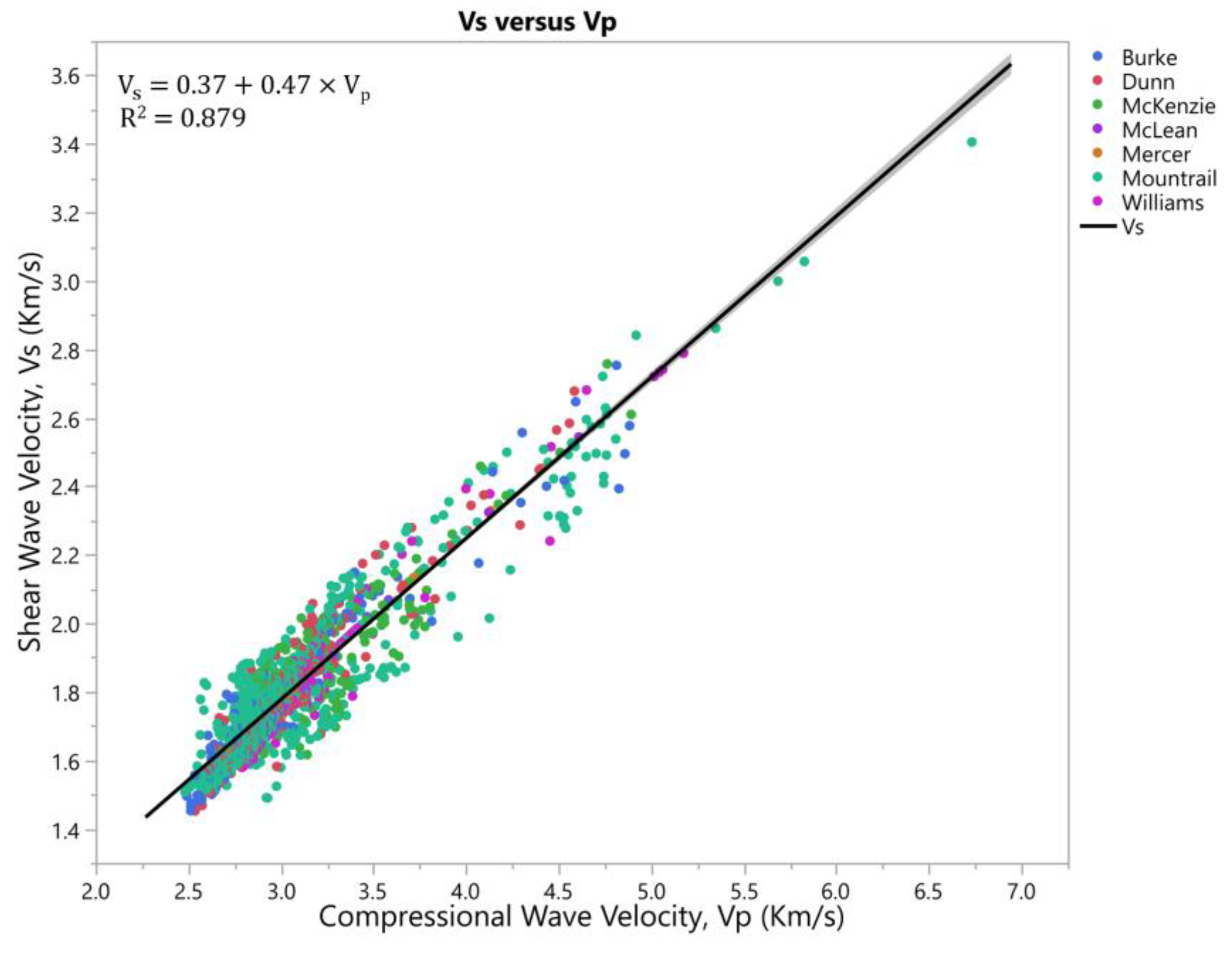
3.1.1. Prediction of Shear Wave Velocity Utilizing Linear Regression Techniques

A linear regression model was obtained in this research additionally to simplify the calculation of shear wave velocity for the Upper and Middle Bakken Formation by just using compressional wave velocity. The linear calculation of shear wave velocity for the Upper and Middle Bakken Formation is of high accuracy and can be used for educational purposes and even for the industry. Figure 13 and Figure 14 shows a linear correlation between shear wave velocity (V_s) and compressional wave velocity (V_p) for the Upper and Middle Bakken Formation achieved in phase I. To determine the level of accuracy for the different models achieved in this paper, coefficient of determination (R²) is used as the primary statistical measure to show the closeness of the predicted data to the actual data. While the adjusted R² was also taken into consideration to determine the accuracy, the difference in the adjusted R² and R² values was negligible because only compressional wave velocity was used as the predictor to predict shear wave velocity in the linear model. If two or more predictors were used to predict shear wave velocity, then the adjusted R² would be a better determining tool of accuracy since it shows how much variance can be explained by a model and the value increases only if the new predictor improves the model [32]. Root Mean Square Error (RMSE) is used as the secondary statistical measure in determining the differences in values between the predicted and the actual. Data Analysis was performed on the data, using the interquartile range technique (IQR) for cleansing out any outliers or heavily skewed data that affect the trendline by removing data points that were 3 standard deviations away from the mean. Along with the IQR technique, scatterplot matrix technique is also used to analyze the data and to detect potential outliers affecting the data trend. A 95% bivariate normal density ellipse is plotted, enclosing approximately 95% of the data points. After cleansing, the linear models achieved an R² of 88% and 72% for the Upper and Middle Bakken respectively, and the derived equation to predict shear wave velocity (V_s) from compressional wave velocity (V_p) linearly is seen below (Equations (3) and (4)). Both shear wave velocity (V_s) and compressional wave velocity (V_p) are in km/s. This correlation is valid for compressional velocity with a range of 2.4 km/s to 5.3 km/s for the Upper Bakken Formation and 4.3 km/s to 5.9 km/s for the Middle Bakken Formation. Derived equation for the Upper Bakken Formation in km/s (Equation (3)):

$${\mathrm{V}}_{\mathrm{s}}=0.37+0.47\times {\mathrm{V}}_{\mathrm{p}}$$

(3)

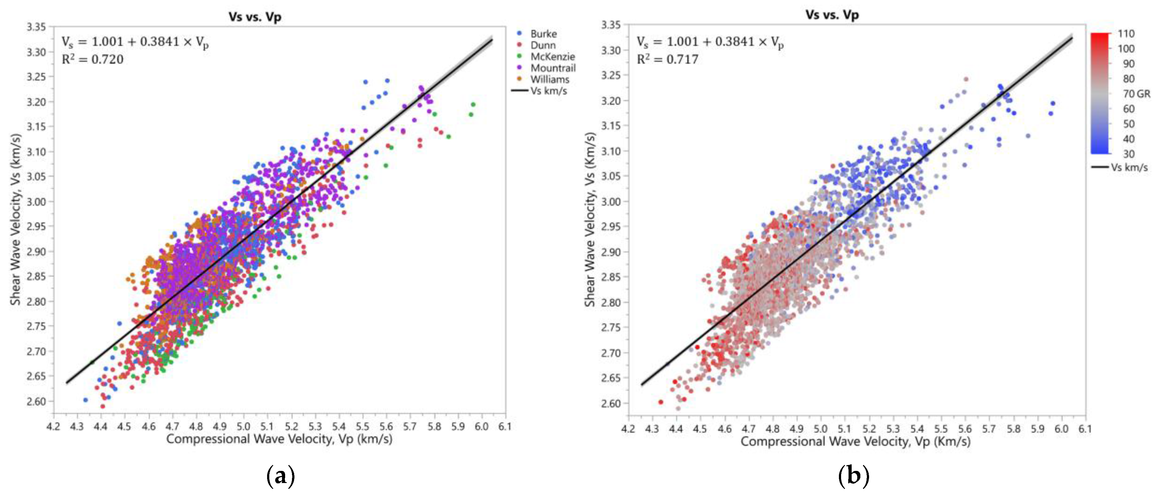
Derived equation for the Middle Bakken Formation in km/s is seen in the equation below (Equation (4)). Figure 14b shows an interesting multivariate analysis and a correlation between the sonic velocities and gamma ray. Shear wave velocity plotted against compressional wave velocity with respect to gamma ray shows a significant decrease in gamma ray readings with an increase in velocity for the Middle Bakken Formation. This is corroborated with multivariate analysis proving that gamma ray has an inverse correlation of 60% with compressional wave velocity, and an inverse correlation of 56% with shear wave velocity for the Middle Bakken Formation. 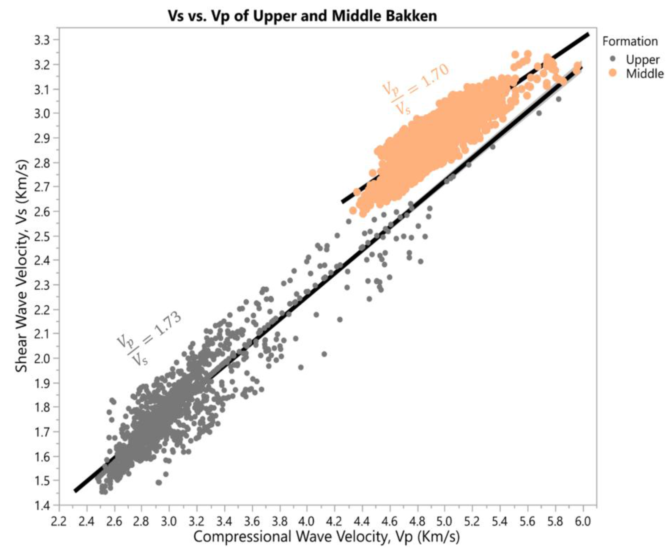Figure 15 shows the V_p/V_s ratio for the Upper and Middle Bakken Formation, with an average V_p/V_s ratio of 1.73 and 1.70 respectively. The significance of the separation is caused due to the large volume of kerogen present in the Upper Bakken Shale’s matrix causing the sonic velocities to be lower than the Middle Bakken’s Sandstone (refer Figure 1).

$${\mathrm{V}}_{\mathrm{s}}=1.001+0.3841\times {\mathrm{V}}_{\mathrm{p}}$$

(4)

Hypothesis testing and statistical inference is also performed, by performing an Analysis of Variance (ANOVA) test on the achieved linear models. This was done by performing an F-test with a confidence level of 95%, which is used to validate the overall significance of the models achieved. The F-hypothesis testing revealed a significant linear relationship between V_p and V_s for both the Upper and Middle Bakken. A T-test is also performed at a confidence interval of 95%, which is used to test for the significance of the intercept and slope coefficients of the linear models achieved. The T-hypothesis testing revealed that the intercept and the slope played a significant contribution to the linear models achieved for the Upper and Middle Bakken.

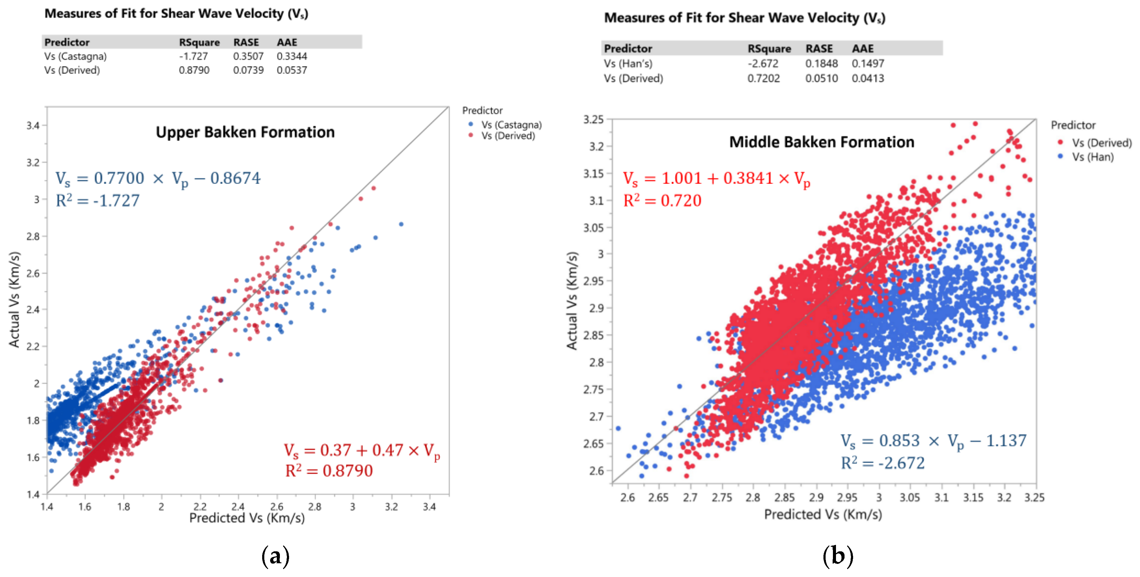
The linear model achieved for the Upper Bakken Shale is compared to Castagna’s mud rock line equation (Equation (5)) in km/s [33,34,35] for shale (water-saturated). Similarly, the linear model achieved for the Middle Bakken Formation is compared to Han’s equation (Equation (6)) for sandstone with porosity lesser than 0.15 [33]. Since the Middle Bakken Formation has very low porosity, it is compared on a similar level to Han’s equation [36,37]. Figure 16 shows the measure of fit for shear wave velocity between Castagna’s equation for shale and the derived equation for the Upper Bakken Shale (left), and Han’s equation for sandstone and the derived equation for the Middle Bakken Sandstone (right). Castagna’s and Han’s equations both have negative R², indicating that the chosen model does not fit well for the Bakken Formation. This suggests that for accurate predictions, sometimes a generalized equation cannot be used on every formation due to the varying lithology in each formation. Similarly, it is important to note that the two achieved linear models in this research can be used for the Upper and Middle Bakken with high degree of certainty of accuracy but may not necessarily work for other formations with the same lithologies and varying properties.

$${\mathrm{V}}_{\mathrm{s}}=0.7700\times {\mathrm{V}}_{\mathrm{p}}-0.8674$$

(5)

$${\mathrm{V}}_{\mathrm{s}}=0.853\times {\mathrm{V}}_{\mathrm{p}}-1.137$$

(6)

3.1.2. Prediction of Shear Wave Velocity Utilizing ANN

Although a linear correlation showed satisfactory results in predicting the shear wave velocity with an R² of 88% and 72% for the Upper and Middle Bakken respectively, a nonlinear correlation utilizing artificial neural networks was also performed to predict shear wave velocity from common conventional well logs such as gamma ray, and bulk density. The results obtained were unsatisfactory and indicated that a pattern was not fully observed. This led to a need of another additional well log, namely compressional wave velocity. In this case, while predicting shear wave velocity, multiple predictors were used to predict it, and hence it would be ideal to use adjusted R² as the determining factor of accuracy. However, to prevent overfitting and overtraining of the data, early stopping and penalty functions were applied to the model and hence the degree of freedom adjustments were not a natural fit for the models [26]. As a result, adjusted R² could not be computed, and the determining factor of accuracy was R² and RMSE. This approach is performed with all the ANN models that follow in this research.

The final model achieved an R² of 94% and 88% for the Upper and Middle Bakken respectively, with it being higher than that of a linear correlation. However, the difference in accuracy of linear fit versus non-linear fit using ANN for the Upper Bakken Shale is negligible. This is because there is not much of heterogeneity variation in the Upper Bakken Shale, as the properties of organic rich shales and source rocks are very uniform throughout their extents. However, with a lot of heterogeneity in the formation, there is a significant difference in the accuracy between linear and non-linear techniques. This is evident in the Middle Bakken Formation comprising of 5 various lithologies, causing high heterogeneity within the formation. In this case, ANN works better than linear techniques, as its pattern recognizing abilities help in creating a relationship between non-linear variables. Thus, for highly heterogenous formations, ANN will work better in forming patterns between highly varying variables, ultimately predicting results with higher and better accuracy.

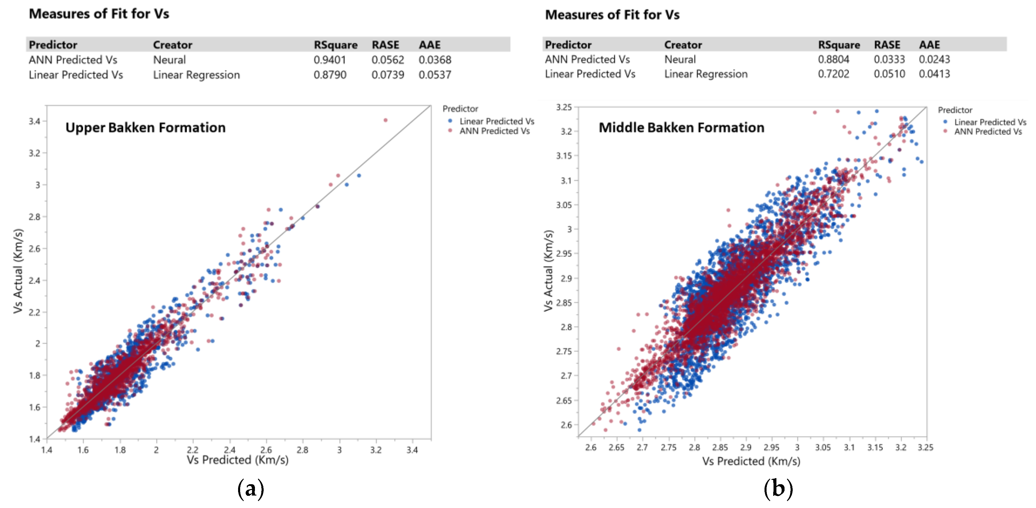
3.1.3. Comparison of Linear and ANN Model to Predict Shear Wave Velocity

Figure 17 shows a decent linear correlation contrasting against the ANN model for the prediction of shear wave velocity. It proves that the ANN model delivers a better line of fit, closely following and centered around the line of best fit. The Root Average Squared Error (RASE) and the Average Absolute Error (AAE) of the ANN model is lower than that of the linear model, thus corroborating the statement that the ANN model fits better than the linear model. Thus, the prediction of shear wave velocity of the remaining 63 wells in phase I was performed using ANN, and the calculation of geomechanical properties for the 112 wells is based on the values of shear wave velocity predicted from neural networks. The complete dataset of calculated dynamic geomechanical properties from phase I are then carried on to phase II, where the geomechanical properties of the Upper and Middle Bakken Formation are predicted from conventional well logs.

3.2. Prediction of Sonic Porosity

In phase II, the initial attempt was to predict geomechanical well logs from basic and commonly used well logs such as gamma ray, and bulk density. The idea was to minimize input logs to predict the output logs to minimize cost and algorithm processing time without compromising the predictive capability and reliability of the model. The initial attempts of achieving satisfactory results was not accomplished, and this led to a need for an additional log as an input. This led to the need to predict sonic porosity from conventional well logs as a prequel to performing the prediction of geomechanical properties of the Upper and Middle Bakken Formation. The parameter of sonic porosity was chosen mainly because it required just basic and commonly used well logs to predict it, and also provided high and accurate predicted results for sonic porosity.

Wyllie’s Method [38], and Raymer-Hunt-Gardner Method as seen in Equations (7) and (8) respectively are widely used for sonic porosity calculation.

$$\mathrm{SPHI}=\frac{\Delta \mathrm{t}-{\Delta \mathrm{t}}_{\mathrm{m}}}{{\Delta \mathrm{t}}_{\mathrm{f}}-{\Delta \mathrm{t}}_{\mathrm{m}}}\times \frac{{\mathrm{H}}_{\mathrm{y}}}{{\mathrm{C}}_{\mathrm{p}}}$$

(7)

$$\mathrm{SPHI}=\mathrm{C}\times \left(\frac{\Delta \mathrm{t}-{\Delta \mathrm{t}}_{\mathrm{m}}}{\Delta \mathrm{t}}\right)$$

(8)

The rock compressional transit time or DTCO (Δt) are obtained from the well logs. For the Upper and Middle Bakken Formation, the transit time for the rock matrix (Δt_m) was assumed to be 56 μs/ft. The interstitial fluid (Δt_f) is assumed to be oil with a transit time of 221.6 μs/ft for the Upper and Middle Bakken. Since Wyllie’s technique (Equation (7)) tends to overestimate porosity in hydrocarbon bearing reservoirs, the operators use empirical corrections such as compaction factor (C_p) of 1, which shows the influence of pore pressure on the sonic porosity equation and is estimated from the sonic response in the nearby shale, and hydrocarbon correction (H_y) was assumed as 0.9 to lessen this error. Similarly, Raymer-Hunt-Gardner equation [39] was also used to calculate the sonic porosity for a few wells of the Upper and Middle Bakken (Equation (8)). The transit time for the rock matrix (Δt_m) was assumed to have the same value of 56 μs/ft as used in Wyllie’s method for the Upper and Middle Bakken. The value of C is an empirical constant and can vary depending on various conditions, and the operators in North Dakota have used a constant value of 0.625 in their calculations of sonic porosity.

Despite the corrections, the calculation of sonic porosity obtained in the well logs are extremely high for the Upper Bakken Formation, and the sonic porosity averages 30%. This is incorrect as the Upper Bakken Shale has very low porosity and permeability. The incorrect and high values of sonic porosity shown on the imported logs is caused primarily due to the uncertainty of empirical corrections used, and also due to the negligence of shale corrections for the Upper Bakken Shale. High kerogen and organic content present in the shale causes variable amounts of low density [40] causing Wyllie’s, and Raymer-Hunt-Gardner’s technique to overestimate the porosity. A Total Organic Carbon (TOC) component can be added to Wyllie’s equation to improve and provide more accurate estimations of sonic porosity for the Upper Bakken Shale. Equation 9, shows Wyllie’s equation modified with the TOC component added to it, to provide a better and clearer estimation of sonic porosity [41].

$$\mathrm{SPHI}=\frac{\left(\Delta \mathrm{t}-{\Delta \mathrm{t}}_{\mathrm{m}}\right)+\left(\frac{{\mathrm{w}}_{\mathrm{TOC}}}{{\mathsf{\rho }}_{\mathrm{TOC}}}\times {\mathsf{\rho }}_{\mathrm{b}}\right)\times \left({\Delta \mathrm{t}}_{\mathrm{m}}-{\Delta \mathrm{t}}_{\mathrm{TOC}}\right)}{{\Delta \mathrm{t}}_{\mathrm{f}}-{\Delta \mathrm{t}}_{\mathrm{m}}}$$

(9)

For the Upper Bakken Shale, the weight fraction of TOC (w_TOC) is provided as seen in Equation (10) below [40].

$${\mathrm{w}}_{\mathrm{TOC}}=\frac{\frac{154.497}{{\mathsf{\rho }}_{\mathrm{b}}}-57.261}{100}$$

(10)

The density of kerogen (ρ_TOC) is assumed to be 1.00 g/cc and the transit time of kerogen (Δt_TOC) is assumed to be 135.47 μs/ft [11].

The incorrect and high values of sonic porosity attributed with the logs for the Upper Bakken Shale have been replaced with the corrected values, and thus, the database now contains the corrected values of sonic porosity. Hence with the data-driven model achieved, accurate estimation of sonic porosity values for future wells will now be predicted by just using basic conventional well logs such as gamma ray, and bulk density. Since phase I was just used as a prequel to phase II, to calculate and complete the database to contain dynamic geomechanical properties and not for any other purpose, sonic porosity will not be calculated using sonic parameters from phase I, even though sonic porosity can be calculated from sonic waves. This research focuses on a cost-effective approach to obtain the sonic porosity, and we do not intend to use sonic logs to achieve sonic porosity. Instead, basic and commonly used logs in the industry which are cost effective such as gamma ray, and bulk density will be used to predict the sonic porosity of the formation using artificial neural networks achieving an accuracy of 87% and 86% for both the Upper and Middle Bakken Formation respectively.

3.3. Prediction of Geomechanical Properties

Finally, upon populating all the missing values in the database, the final database consists of the input independent variables Depth, Gamma Ray (GR), Bulk Density (RHOB), Sonic Porosity (SPHI), and the output dependent variables Dynamic Young’s Modulus (E), Dynamic Poisson’s Ratio (v), Dynamic Bulk Modulus (K), Dynamic Shear Modulus (G), and Minimum Horizontal Stress (σ_min) for each of the 112 wells.

Overall, the models obtained from neural networks achieved R² over 90%. This was possible by cascading technique instead of multiple output neuron technique. By cascading technique, the output of the geomechanical property achieved from the previous model was used as an input along with the conventional well logs to predict the next geomechanical property in the next model. The geomechanical property first predicted was based on trial and error, and the output that gave a higher accuracy was predicted first. The output was then used as an input for the next model and the next geomechanical property to be predicted was again based on trial and error. The geomechanical property output giving a higher accuracy was selected as the second geomechanical property to be predicted. This process continued and until all five geomechanical properties were obtained [21] for each formation. With this approach, the results kept improving for every geomechanical property generated, and ultimately, a highly reliable model for predicting minimum horizontal stress from conventional well logs; achieving an R² of 98% for the Upper and Middle Bakken Formation.

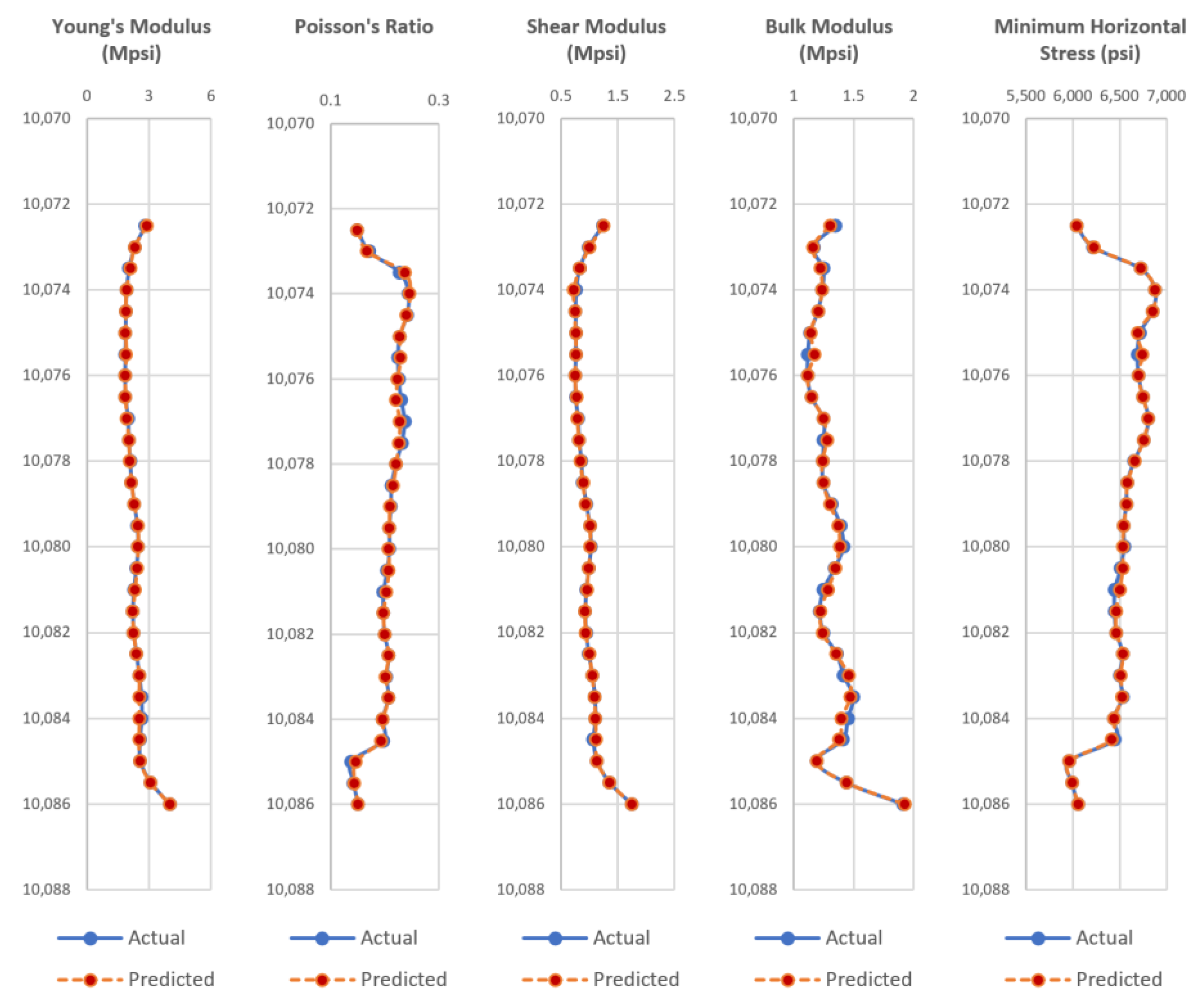
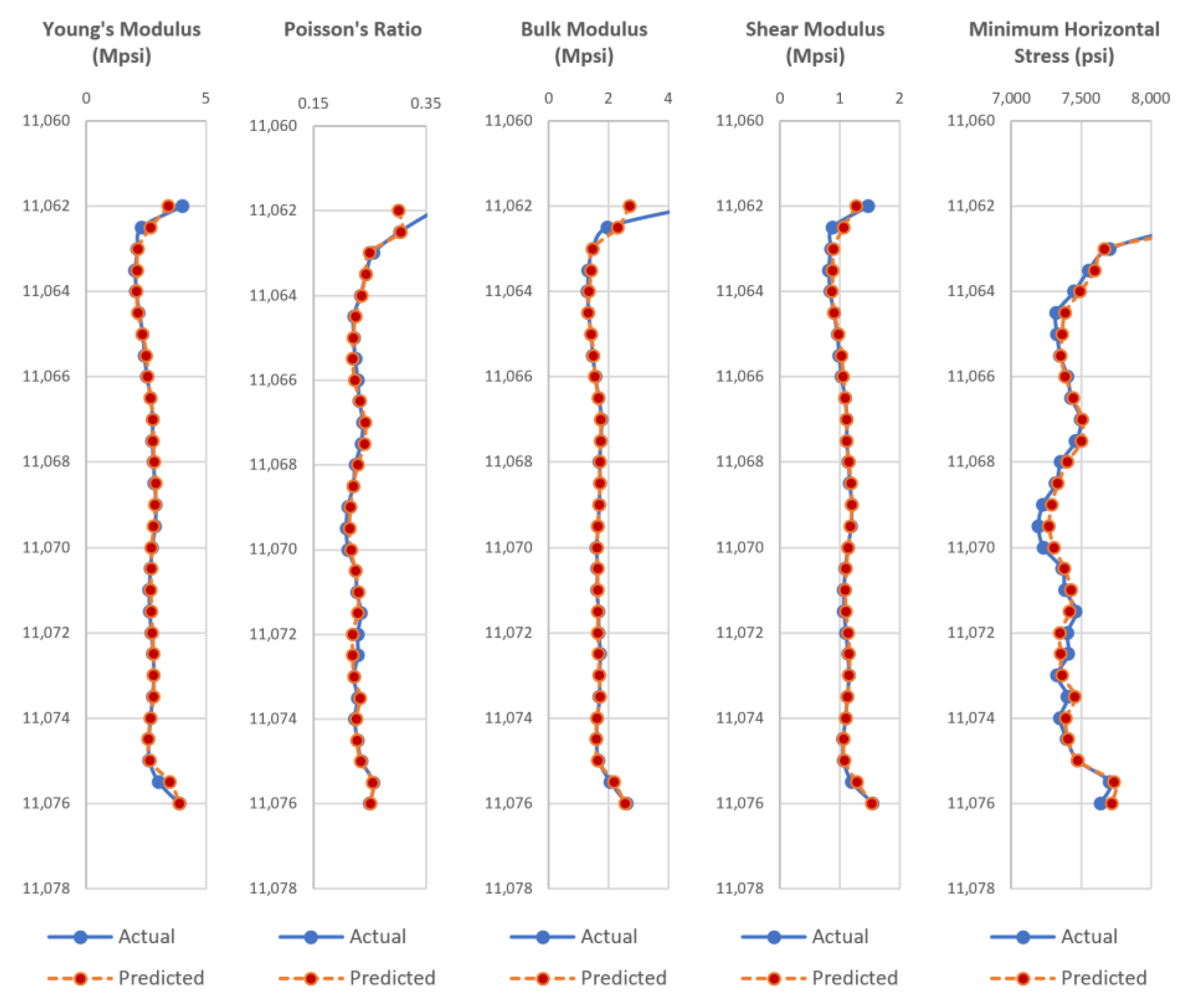
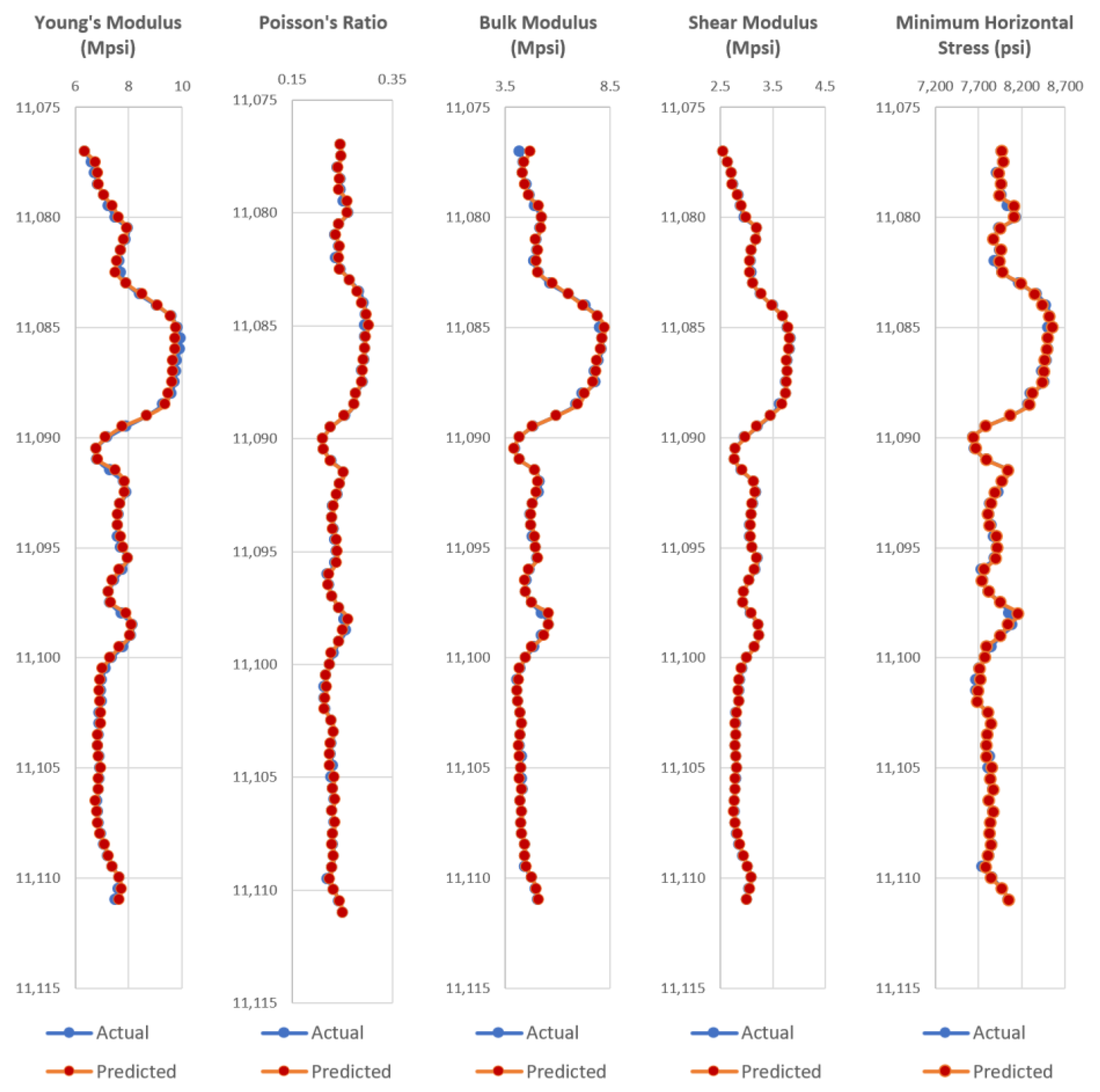
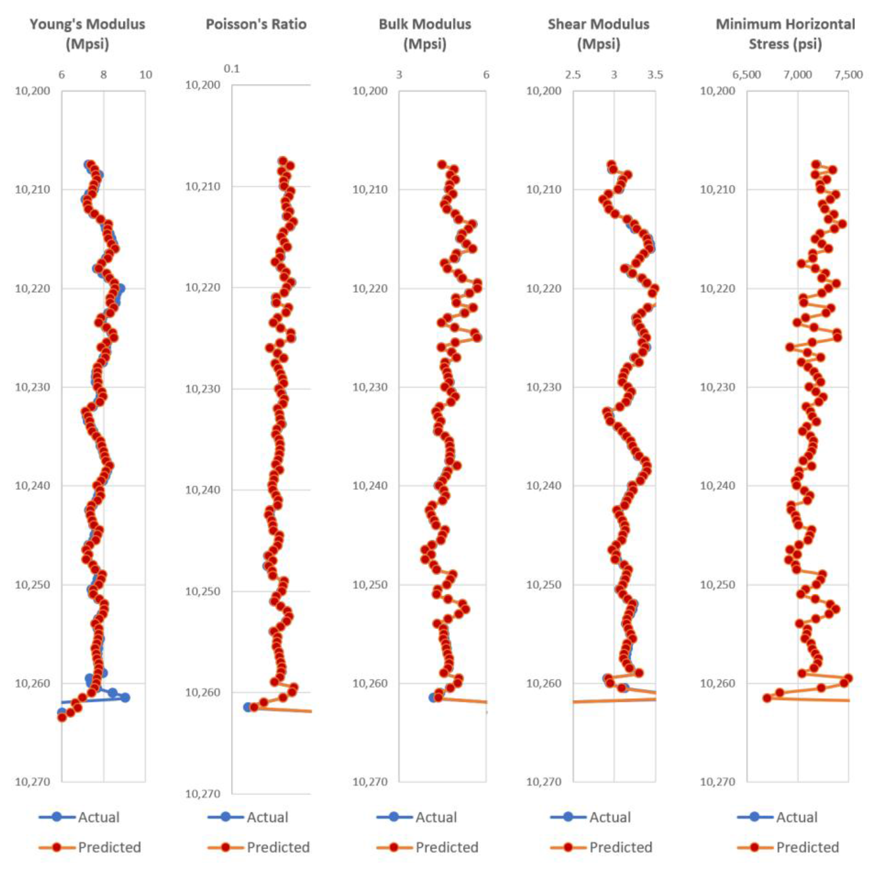
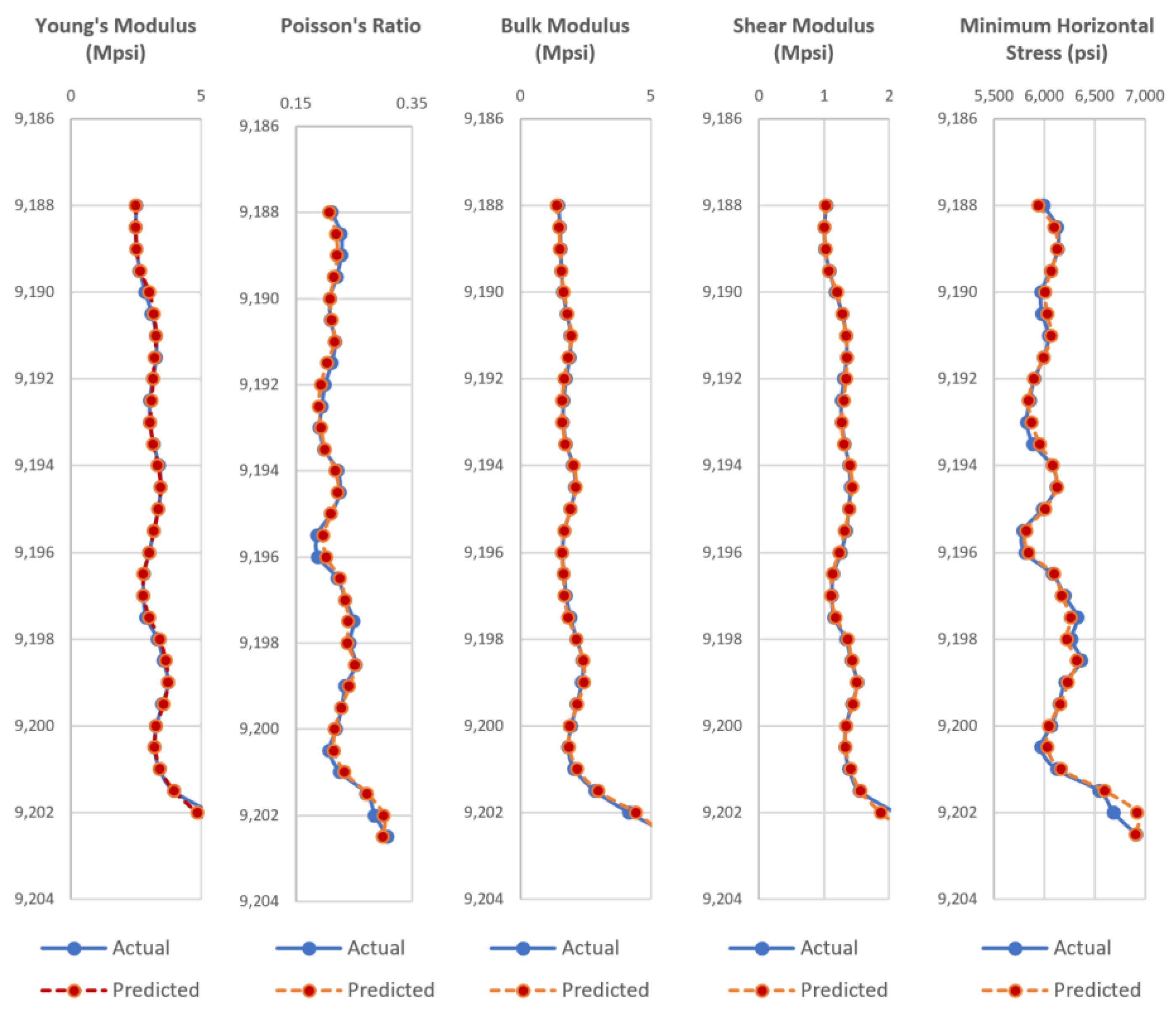
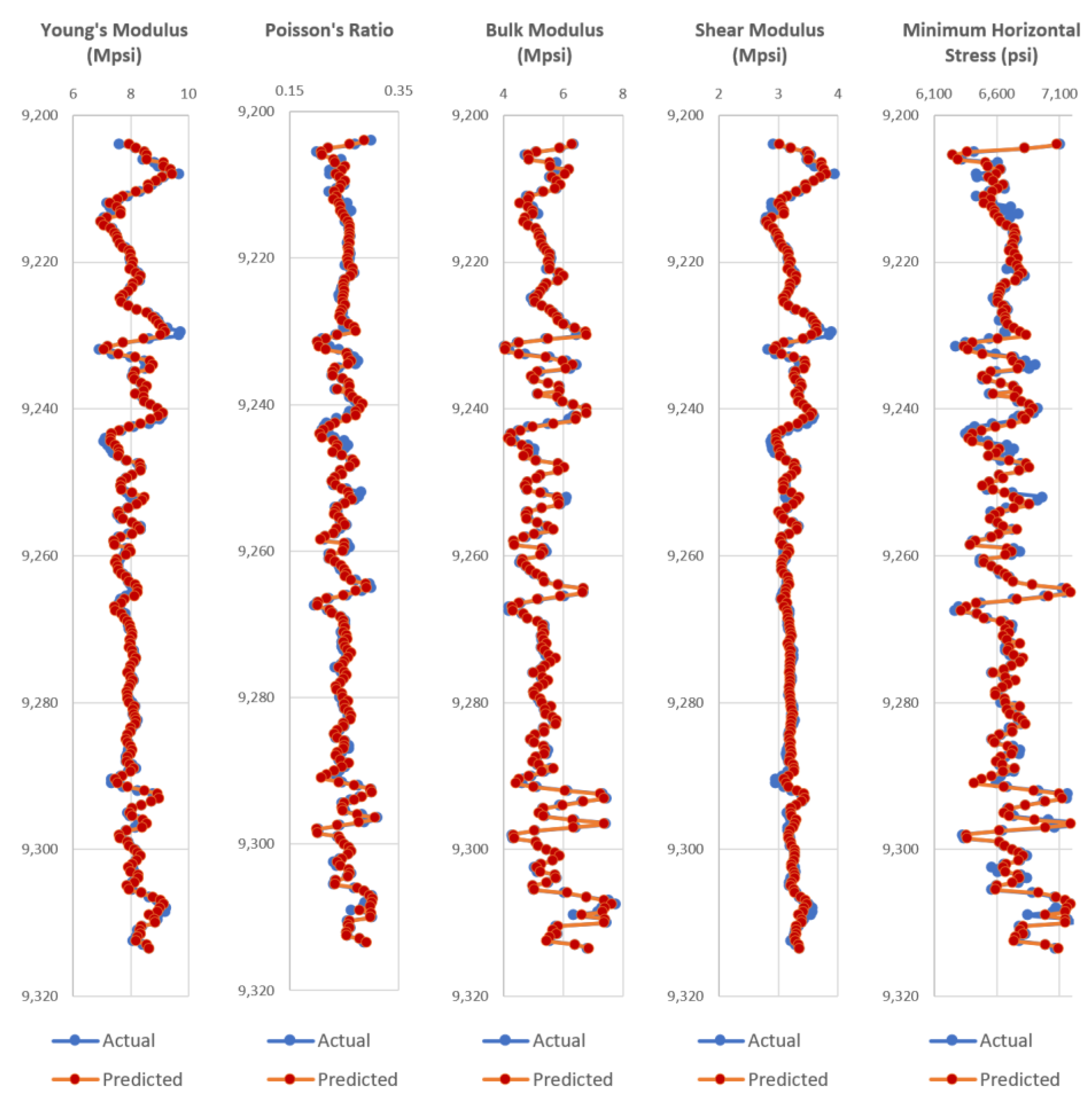
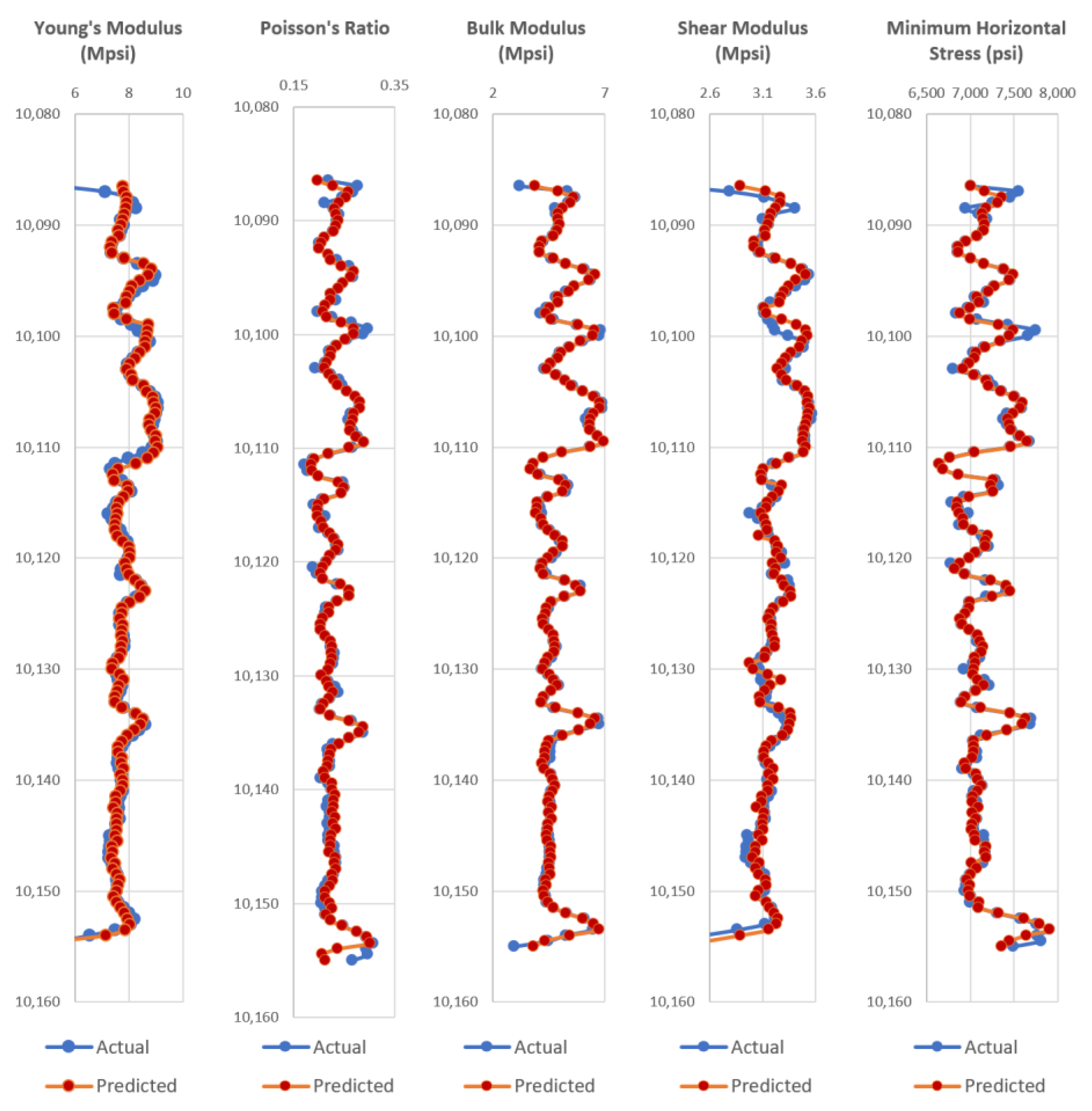
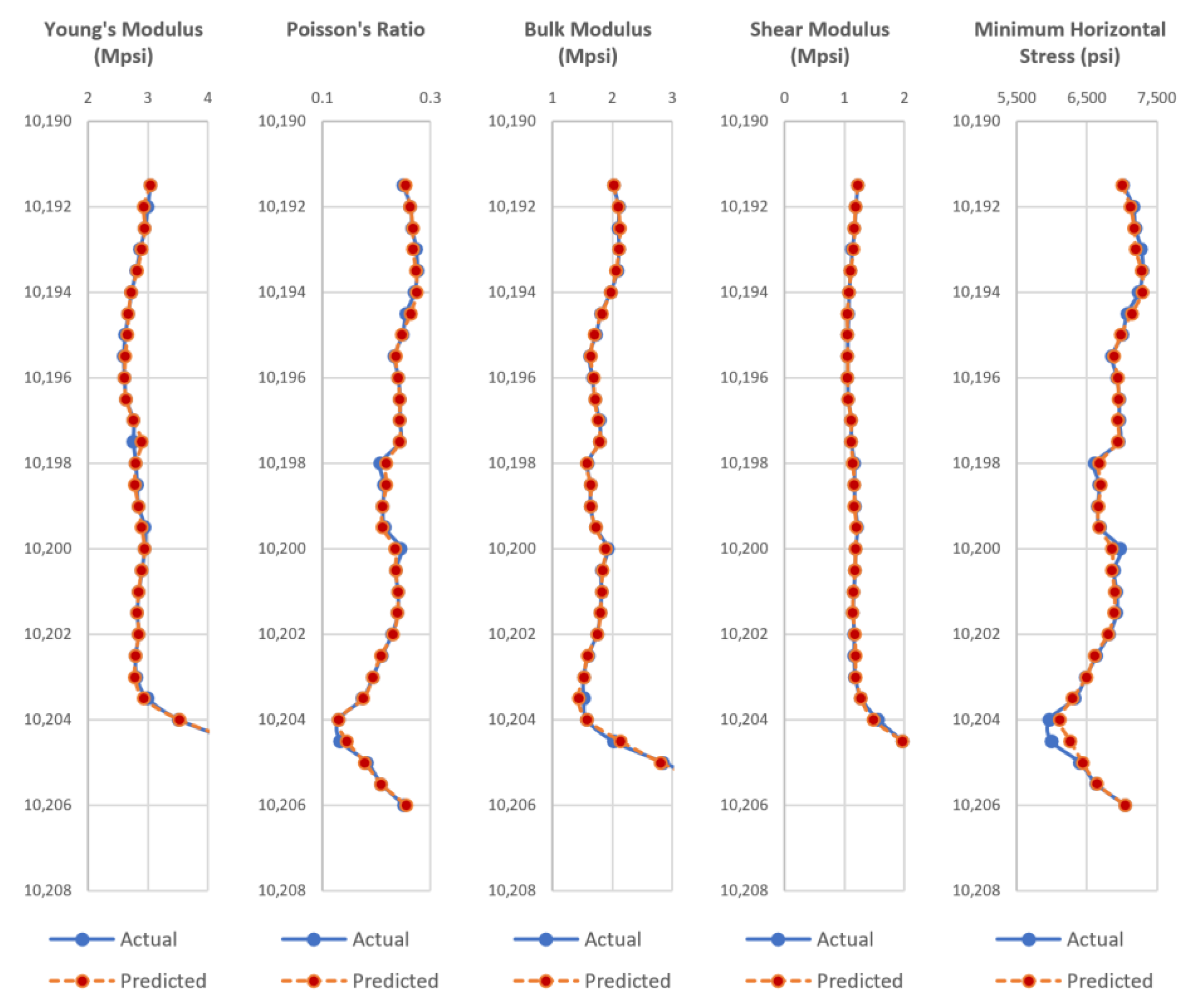
To prove the efficacy of the ANN models achieved, it is tested on 5 additional test wells spread across the 5 major producing counties in North Dakota. The data from the 5 wells were not used in the dataset to train the ANN models achieved in phase II, thus highlighting the efficacy of the ANN models achieved in this research. In Appendix A, the test wells actual dynamic geomechanical well logs are compared to the predicted dynamic geomechanical properties obtained from the ANN models in phase II. 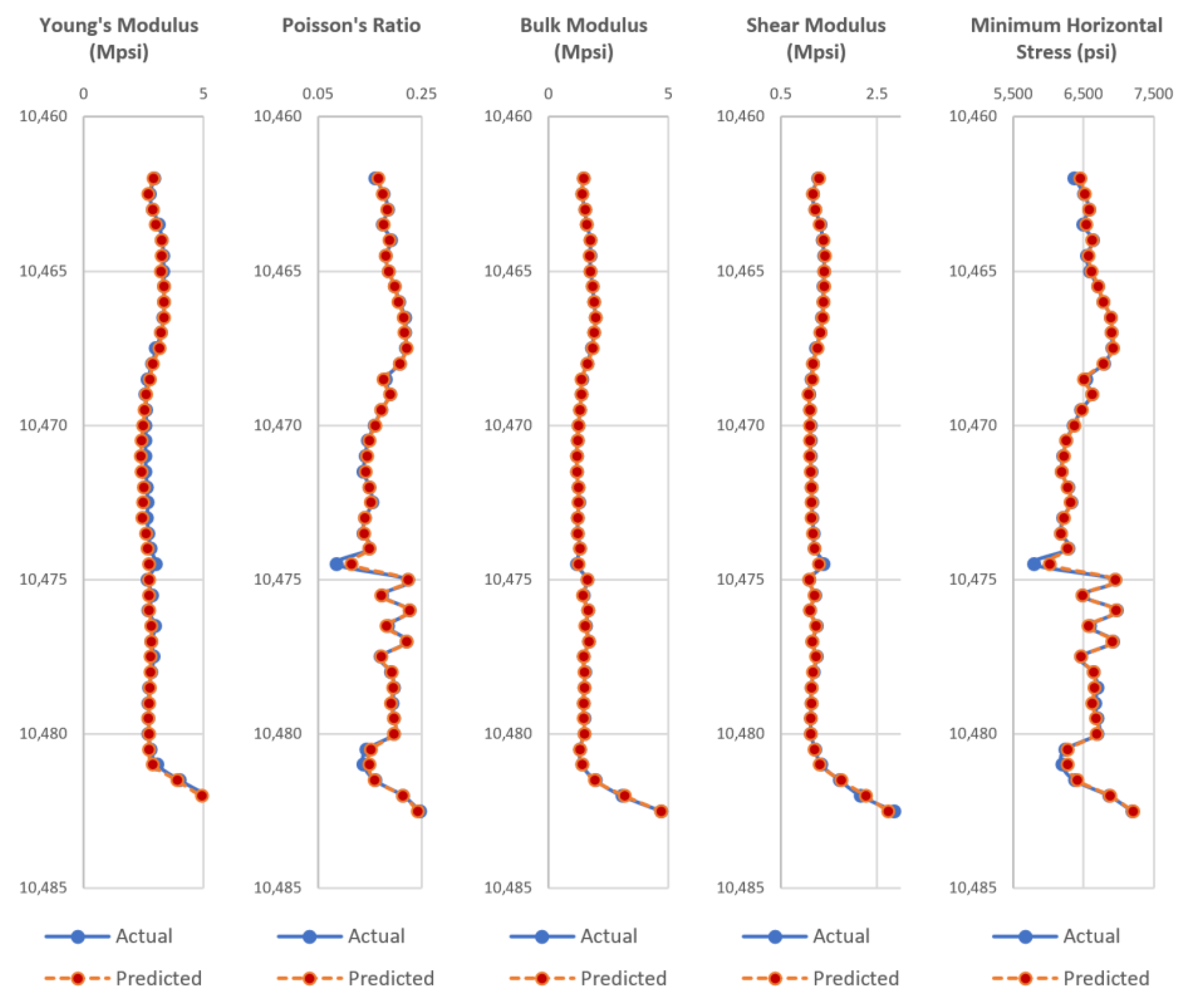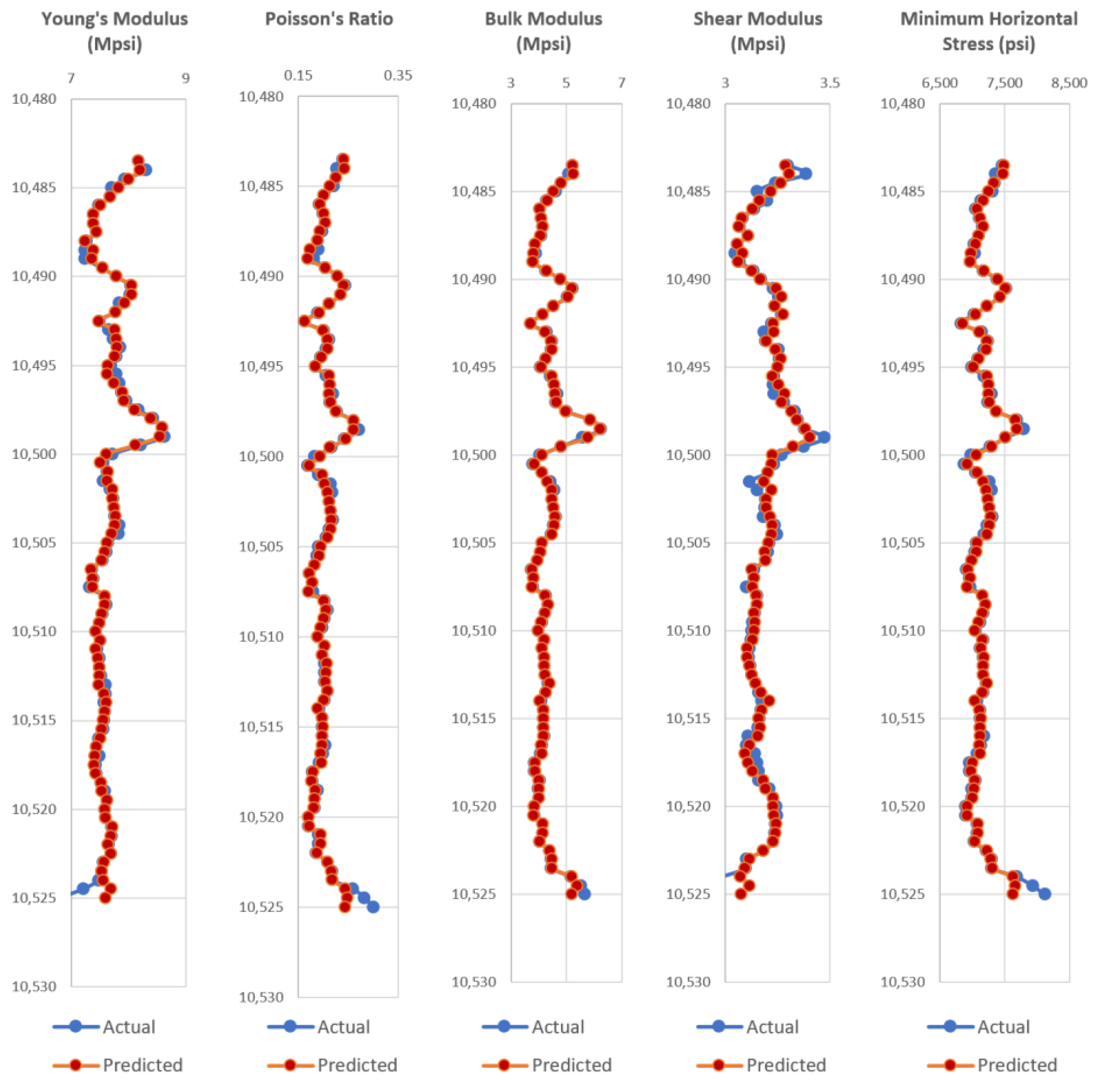Figure A1, Figure A2, Figure A3, Figure A4, Figure A5, Figure A6, Figure A7, Figure A8, Figure A9 and Figure A10 show actual dynamic geomechanical logs and predicted geomechanical properties along with depth for each of the five test wells of the Upper and Middle Bakken Formation each. The outcome of using the data-driven model on randomly selected test wells is highly accurate and proves the reliability and efficacy of the model in predicting geomechanical properties of future wells for the Upper and Middle Bakken Formation.

4. Conclusions

This research shows that statistical methods along with artificially intelligent supervised machine learning data models have successfully aided in the achievement of three outcomes. The first outcome is the prediction of shear wave velocity using linear and non-linear techniques. A new linear correlation to determine shear wave velocity is proposed for the Bakken Formation with accuracies of 88% and 72% for the Upper and Middle Bakken Formation respectively. However, the goal of the research to use supervised ANN models to predict shear wave velocity was a success, with estimations of higher accuracies of 94% and 86% for the Upper and Middle Bakken Formation respectively. The second outcome is the prediction of sonic porosity from basic conventional well logs utilizing ANN. Instead of using expensive sonic logs to calculate the sonic porosity, this research shows an economic alternative to predict sonic porosity by just using commonly used conventional well logs, with estimations of significantly high accuracies of 87% and 86% for the Upper and Middle Bakken Formation respectively. To get better estimations of sonic porosity for the Upper Bakken Shale that contains large amounts of kerogen, the impact of kerogen on sonic porosity was also accounted for, which resulted in more accurate estimations of sonic porosity for the Upper Bakken Shale.

Ultimately: data-driven models are generated that predict geomechanical properties of the Bakken Formation from just basic and commonly used conventional well logs with an accuracy greater than 90%, and a very high estimation of minimum horizontal stress of 98% accuracy. This is tested and proven on 5 additional randomly chosen test wells in North Dakota, whose data were not included in the original database, thus giving us confidence and assurance that the data models work and can predict geomechanical properties for future wells of the Bakken Formation in North Dakota. Altogether, this study shows the benefits of using artificially intelligent supervised machine learning techniques as an approach in obtaining valuable information for oil and gas operators. In today’s era, where cost savings is one of the primary objectives for oil and gas operators, the integration of statistical techniques along with supervised artificially intelligent methods in the oil and gas industry is potentially a smart technique in obtaining valuable information about reservoir properties, ultimately leading to improvements in performance, efficiency, and profitability for oil and gas operators.