Research on Improved VSG Control Algorithm Based on Capacity-Limited Energy Storage System

Abstract

A large scale of renewable energy employing grid connected electronic inverters fail to contribute inertia or damping to power systems, and, therefore, may bring negative effects to the stability of power system. As a solution, an advanced Virtual Synchronous Generator (VSG) control technology based on Hamilton approach is introduced in this paper firstly to support the frequency and enhance the suitability and robustness of the system. The charge and discharge process of power storage devices forms the virtual inertia and damping of VSG, and, therefore, limits on storage capacity may change the coefficients of VSG. To provide a method in keeping system output in an acceptable level with the capacity restriction in a transient period, an energy control algorithm is designed for VSG adaptive control. Finally, simulations are conducted in DIgSILENT to demonstrate the correctness of the algorithm. The demonstration shows: (1) the proposed control model aims at better system robustness and stability; and (2) the model performs in the environment closer to practical engineering by fitting the operation state of storage system.

1. Introduction

In recent years, penetration of distributed generation (DG) in power systems is increasing rapidly, accompanied with the reduction of total system inertia. To play their potential fully and reduce their negative effects at the same time, specific functionalities are designed for the converter interfacing DG and power grid [1,2,3,4]. Virtual synchronous generator (VSG) technology [5,6], which imitates the output characteristic of synchronous generator (SG) to enhance the stability of power grid, is one of the effective methodologies and attracting more and more attention.

In the project of Virtual Synchronous Machines (VSYNC) in Poland, an idea named VSG was put forward the first time, aiming at making the converter imitate the mechanical equation for a more stable grid frequency [7]. A further study in excitation control was introduced later, completing and developing the VSG system [8]. However, since the immaturity of the early VSG technology, the dynamic response of the systems are commonly slow and accompanied with slight oscillations.

Small-signal modeling is one of the mainstream methods in linear system analysis and it is widely used in VSG for system stabilization. Comparisons are illustrated in [9] between droop control and VSG control. Superiority of VSG has been proved by comparing dynamic responses via small-signal modeling and state equations. In [10], every specific elements of the inverter control modeling are listed and analyzed. The corresponding small-signal model is then established for obtaining controller sensitivity and revealing the effects of different parameters towards VSG system.

One of the merits of VSG compared to the SG is that the former one enjoys flexible parameters selection. Analysis in [11] shows that the virtual inertia enjoys self-adaption depending on disturbance. In [12,13], an adaptive alternating inertial control algorithm is introduced. They verify the validity that the VSG can work at the state of negative inertia, being more flexible and adjustable than the SG. With a further study in [14,15], virtual inertia varies to meet the demands according to advanced control algorithm rather than a fixed coefficient in [12,13]. Based on the studies above, VSG is commonly regarded as the second-order system for simplification by neglecting parts of SG, resulting in a less precise modeling. In this paper, a more accurate model is established and performs better in mimicking SG characteristics.

The generalized Hamilton function method enjoying its superiority in nonlinear system research for the merits in depicting the dynamic energy flow [16,17,18]. The technology is attracting more and more attention gradually. In [19], a fifth-order model of the SG is established with an energy-based Lyapunov function. In [20,21], a further study is conducted that the modeling of generator integrated AVR (Automatic Voltage Regulator) and PSS (Power System Stabilization) shows the superiority of the Hamilton approach in improving system robustness and stabilization. Considering the superiority, an advanced control algorithm based on the Hamilton approach is applied to the VSG for better suitability and robustness. Energy-based control laws are conducted via applying the Hamiltonian approach to valving control and excitation system in this paper.

Electronic inverters fail to contribute inertia or damping to power grid, leading to a necessity that the energy storage devices should be equipped to compensate the power vacancy [22]. In current study, DG and storage devices are commonly simplified as DC power sources. In [23,24], conclusions can be drawn that it is the charge and discharge progress of the storage devices that form the virtual inertia. In [25], an optimal control strategy of the storage systems by setting the VSG’s output active power depending on the grid frequency deviation is put forward. In [26], storage devices act as power buffers to compensate power shortage in short-term impact for transient stability. Existing studies focus on the significance of storage devices and binary control strategies between VSG and storage devices, neglecting the connections between the storage devices and the VSG coefficients. Furthermore, storage capacity is generally considered as unlimited in theoretical analysis, being considerably different from the situation in practical engineering. Given the insufficiencies, corresponding analyses and solutions are proposed.

Contributions of this paper are listed as follows:

• A fourth-order model of VSG, being more detailed and accurate in mimicking SG, is established. Based on the second-order model, the steam-valving system and excitation system are added, taking the coordination between the two systems into consideration while avoiding the complicated transition period.
• A nonlinear control method, Hamilton approach is applied to VSG for better system suitability and stability. Control laws are deduced and the system enhancements are illustrated.
• Small-signal model is established for the obtaining boundaries of VSG coefficients.
• Relations between the capacity limits of storage devices and the VSG coefficients, such as the virtual inertia and damping, are discussed. An adaptive VSG control is designed via the energy control algorithm for accelerating the recovery from the transient period.

This paper is organized as follows: In Section 2, VSG modeling aspects are illustrated. Energy controller unit is then conducted in Section 3. Simulations are given in Section 4. Conclusions are drawn in Section 5.

2. Virtual Synchronous Generator Modeling Based-On the Hamilton Approach

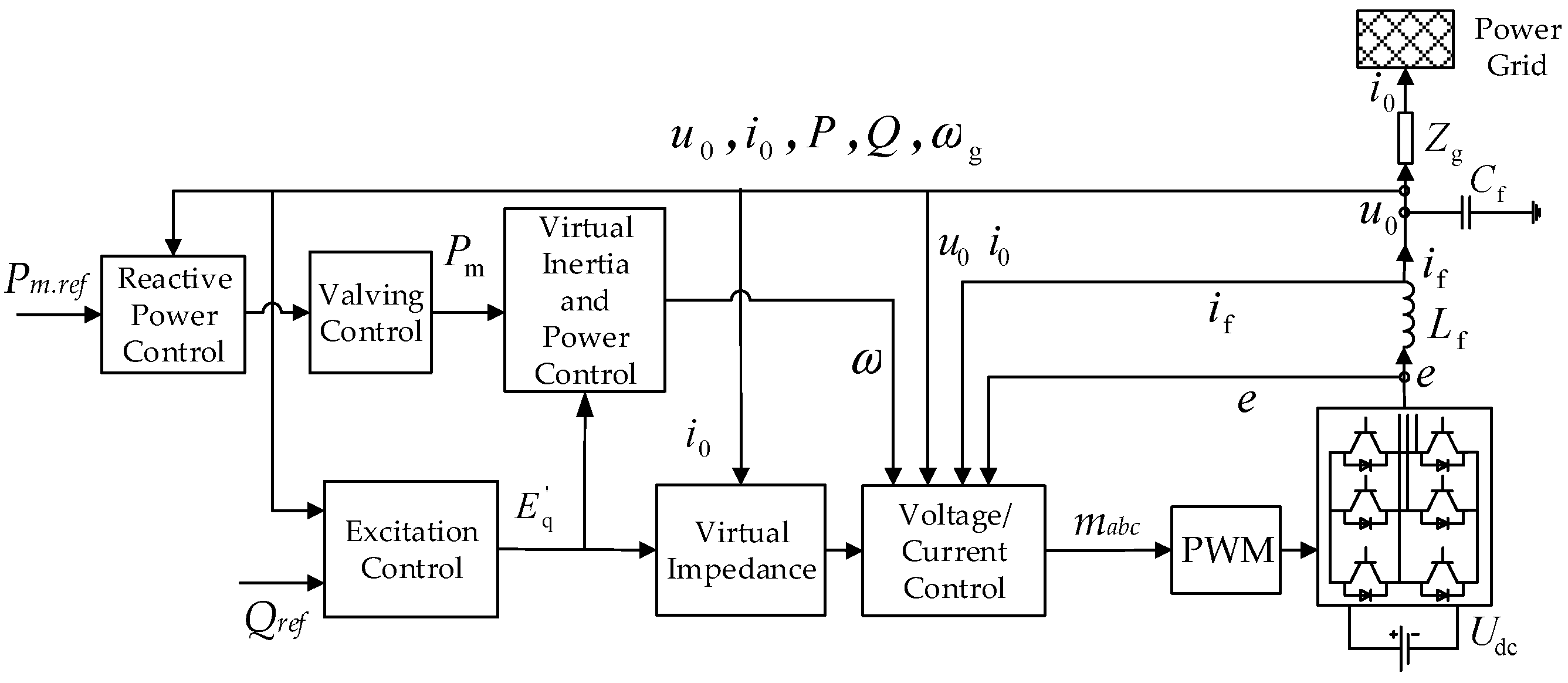
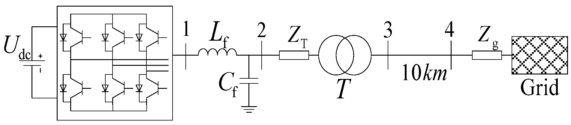
2.1. VSG Control System Overview

Detailed classification methods in VSG modeling are illustrated in [27] based on the order of SG modeling. In this paper, a fourth-order model contains the steam-valving system and steam turbine generator excitation system is built, performing better in revealing the coordination between the valve and the exciter. Therefore, a control algorithm based on energy function is deduced by making use of Hamilton control system with virtual synchronous generator excitation (VSG) system and turbine valve control, in which the physical significance is clearer than before. Figure 1 depicts the overall block diagram of VSG control strategy.

As indicated in Figure 1, U_dc, which is assumed that the dc-link of the VSG is connected to an energy storage unit or to a source with sufficient available buffer capacity, acts as the virtual prime mover. The inductance of the filter inductor is L_f and filter capacitor is C_f. The output voltage for the converter is denoted by e, representing the transient voltage of synchronous generator while the current reference, tracked by the controller, is given by i_f. Meanwhile, u₀ is the voltage at the filter capacitors and i₀ is the current flowing into the grid or load equivalent, which are equivalent to the terminal voltage and current of stator winding of a synchronous generator (SG), making the dynamic parameters at grid connection point, such as u₀, i₀, f and P_e, mimic the characteristic of a SG.

2.2. VSG Modeling Based on Dissipative Hamilton Theory

VSG shares the same mathematical model as the SG, and its mechanical equations are given as Equation (1)

$$\{\begin{array}{l}\dot{\delta }=\omega -{\omega }_0\\ \dot{\omega }=\frac{{\omega }_0}{M}(P_m-P_e)-\frac{P_D}{M}=\frac{{\omega }_0}{M}(P_m-P_e)-\frac{D(\omega -{\omega }_0)}{M}\end{array},$$

(1)

where D is damping, M is virtual inertia, P_e is the system output power, P_m the mechanical power, ω the angular velocity, ω₀ the angular velocity references.

The mechanical power P_m considering the steam-valving is given as Equation (2).

$${\dot{P}}_m=\frac{1}{T_s}(-P_m+P_{m0})+\frac{1}{T_s}{\mu }_g,$$

(2)

where T_s represents the time constant, P_m0 is the mechanical power reference and μ_g the valving control signal.

The output power P_e of the VSG is given as Equation (3).

$$P_e=\frac{E_q^{\text{'}}{U}_s\sin \delta }{x_{d\sum }^{\text{'}}},$$

(3)

where δ is the power angle of VSG, E_q’ the transient electrodynamic force (E.M.F) on q-axis, U_s the voltage of infinite bus-system and x’_dΣ the total stator-winding reactance of d-axis.

The excitation control equation is given as Equation (4).

$$T_{d0}\frac{d{E}_q^{\text{'}}}{dt}=U_f-E_q^{\text{'}}-(X_d-X_d^{\text{'}})i_d,$$

(4)

where T_d0 is the time constant in excitation winding, x_d the self-inductance resistance, x_dΣ the total stator-winding reactance of d axis and U_f the excitation voltage. i_d in Equation (4) are noted as Equation (5).

$$i_d=\frac{E_q-U_s\cos \delta }{x_{d\sum }}=\frac{E_q^{\text{'}}-U_s\cos \delta }{x_{d\sum }^{\text{'}}}.$$

(5)

According to Equations (1)–(5), system state equations are given in Equation (6):

$$\{\begin{array}{l}\dot{\delta }=\omega -{\omega }_0\\ \dot{\omega }=\frac{{\omega }_0}{M}{P}_m-\frac{D(\omega -{\omega }_0)}{M}-\frac{{\omega }_0{U}_s}{M{x}_{d\sum }^{\text{'}}}{E}_q^{\text{'}}\sin \delta \\ {\dot{E}}_q^{\text{'}}=-\frac{x_{d\sum }}{x_{d\sum }^{\text{'}}{T}_{d0}}{E}_q^{\text{'}}+\frac{(x_d-x_d^{\text{'}})U_s}{x_{d\sum }^{\text{'}}{T}_{d0}}\cos x_1+\frac{1}{T_{d0}}{E}_f\\ {\dot{P}}_m=-\frac{1}{T_s}{P}_m+\frac{1}{T_s}{P}_{m0}+\frac{1}{T_s}{\mu }_g\end{array},$$

(6)

where x_{1 =} δ, x_{2 =} ω − ω₀, x_{3 =} E_q’, x₄ = P_m and Equation (6) can be transformed into Equation (7)

$$\{\begin{array}{l}{\dot{x}}_1=x_2\\ {\dot{x}}_2=\frac{{\omega }_0}{M}{x}_4-\frac{D}{M}{x}_2-\frac{{\omega }_0{U}_s}{M{x}_{d\sum }^{\text{'}}}{x}_3\sin x_1+w_1\\ {\dot{x}}_3=-p_1{x}_3+p_2\cos x_1+u_1+w_2\\ {\dot{x}}_4=-\frac{1}{T_s}{x}_4+\frac{1}{T_s}{P}_{m0}+u_2+w_3\end{array}.$$

(7)

In Equation (7), p₁ and p₂ are parameters with perturbation, u₁ and u₂ are system input and w₁, w₂ and w₃ disturbances of the system. After obtaining the equilibrium points, Equation (7) can be transformed to Equation (8). Details are shown in Equation (9).

$$\dot{X}=(J-R)\nabla H(x)+g_{1}v+g_{2}w,$$

(8)

where

$$\begin{array}{c}\nabla H(x)=\left[\begin{array}{c}\frac{\partial H(x)}{\partial x_1}\\ \frac{\partial H(x)}{\partial x_2}\\ \frac{\partial H(x)}{\partial x_3}\\ \frac{\partial H(x)}{\partial x_4}\end{array}\right]=\left[\begin{array}{c}{a}_{23}{x}_3\sin x_1\frac{a_{21}{a}_{42}}{a_{41}}\\ x_2\\ \frac{p_1{a}_{23}}{p_2}{x}_3\frac{a_{23}}{p_2}{U}_{f0}-a_{23}{x}_3\cos x_1\\ a_{21}{x}_4-\frac{a_{21}{a}_{42}}{a_{41}}\end{array}\right],\\ J=\left[\begin{array}{cccc}0& 1& 0& 0\\ -1& 0& 0& 1\\ 0& 0& 0& 0\\ 0& -1& 0& 0\end{array}\right]R=\left[\begin{array}{cccc}0& 0& 0& 0\\ 0& a_{22}& 0& 0\\ 0& 0& \frac{p_2}{a_{23}}& 0\\ 0& 0& 0& \frac{a_{41}}{a_{21}}\end{array}\right]g_1=\left[\begin{array}{cc}0& 0\\ 0& 0\\ 1& 0\\ 0& 1\end{array}\right]g_2=\left[\begin{array}{ccc}0& 0& 0\\ 1& 0& 0\\ 0& 1& 0\\ 0& 0& 1\end{array}\right].\end{array}$$

(9)

Equation (8) is a dissipative Hamilton approach where g₁(x), g₂(x) and v are all column vectors of m dimension and H(x) is regarded as the Hamilton function. Matrix J is antisymmetric and matrix R is positive semidefinite.

Parameters in Equations (8) and (9) are shown in Equations (10) and (11).

$$\{\begin{array}{l}\begin{array}{lll}{a}_{21}=\frac{{\omega }_0}{M}\hfill & a_{22}=\frac{D}{M}\hfill & a_{23}=\frac{{\omega }_0{U}_{\mathrm{s}}}{M{x}_{\mathrm{d}\sum }^{\prime }}\hfill \end{array}\hfill \\ \begin{array}{cc}{a}_{41}=\frac{1}{T_{\mathrm{s}}}& a_{42}=\frac{1}{T_{\mathrm{s}}}{P}_{\mathrm{m}0}\end{array}\hfill \\ \begin{array}{cc}{p}_1=\frac{x_{\mathrm{d}\sum }}{x_{\mathrm{d}\sum }^{\prime }{T}_{\mathrm{d}0}}& p_2=\frac{(x_{\mathrm{d}}-x_{\mathrm{d}}^{\prime })U_{\mathrm{s}}}{x_{\mathrm{d}\sum }^{\text{'}}{T}_{\mathrm{d}0}}\end{array}\hfill \end{array},$$

(10)

where v₁ and v₂ are the inputs after the introduction of state feedback, whose relations with u₁ and u₂, the original input of the system, can be given by Equation (10).

$$\{\begin{array}{l}{v}_1=u_1-U_{\mathrm{f}0}=\frac{1}{T_{\mathrm{d}0}}{U}_{\mathrm{f}}-U_{\mathrm{f}0}\hfill \\ v_2=u_2-x_2=\frac{1}{T_{\mathrm{s}}}{\mu }_{\mathrm{g}}-x_2\hfill \end{array}.$$

(11)

In Equation (10), U_f is the voltage of the excitation system, defined by the equation U_f = U_f0 + u_f, in which u_f is the regulation of the excitation voltage.

Equation (9) fits in the form of the dissipative Hamilton system, which can be regarded as one of the Hamilton approaches of VSG. Then, Hamilton function can be deduced after solving $\nabla$H(x) in Equation (9) out and noted as Equation (12) [28,29].

$$H(X,p_1,p_2)=-2a_{23}{x}_3\cos x_1-\frac{a_{21}{a}_{42}}{a_{41}}{x}_1+\frac{x_2^2}{2}+\frac{a_{21}{x}_4^2}{2}-\frac{a_{21}{a}_{42}}{a_{41}}{x}_4+\frac{p_1{a}_{23}}{2p_2}{x}_3^2-\frac{a_{23}{U}_{f0}}{p_2}$$

(12)

A penalty function z, an interference suppression level γ and a weight matrix r(X) are firstly defined and given in Equation (13).

$$\{\begin{array}{l}z=r{g}_1^T(X,p)\nabla H(X,p_0)\\ r(X)=diag(r_1,r_2)>0\end{array}.$$

(13)

If it satisfies the condition in Equation (14) in any circumstances,

$$\{\begin{array}{l}z\equiv 0,g_2^T\nabla H\equiv 0\\ R+\frac{1}{2{\gamma }^2}[g_1{g}_1^T-g_2{g}_2^T]\ge 0\end{array}.$$

(14)

Then, the control law of VSG based on Hamilton approach is given in Equation (15):

$$\{\begin{array}{l}\left[\begin{array}{c}{v}_1\\ v_2\end{array}\right]=-\frac{1}{2}{r}^T(X)r(X)g_1^T\nabla H-\frac{1}{2{\gamma }^2}{g}_1^T\nabla H-{\varphi }^T\theta \\ \dot{\theta }=Q\varphi g_1^T\nabla H\end{array},$$

(15)

where $\theta$ is an intermediate variable.

Details are shown in Equation (15) when parameters are substituted to Equation (16).

$$\{\begin{array}{l}\dot{\theta }=Q[-\frac{{\omega }_0{U}_s}{M{x}_{d\sum }^{\text{'}}}{E}_q^{\text{'}}\cos \delta +\frac{{\omega }_0{U}_s{x}_{d\sum }}{M{x}_{d\sum }^{\text{'}}(x_d-x_d^{\text{'}})}{(E_q^{\text{'}})}^2]\\ u_f=T_{d0}{U}_{f0}-T_{d0}{E}_q^{\text{'}}\theta +\frac{T_{d0}}{2}(r_1^2+\frac{1}{{\gamma }^2})\left[\frac{{\omega }_0{U}_s}{M{x}_{d\sum }^{\text{'}}}\cos \delta -\frac{{\omega }_0{E}_q^{\text{'}}{x}_{d\sum }}{M{x}_{d\sum }^{\text{'}}(x_d-x_d^{\text{'}})}\right]\\ {\mu }_g=T_s(\omega -{\omega }_0)+\frac{T_s{\omega }_0}{2M}(r_2^2+\frac{1}{{\gamma }^2})(P_{m0}-P_m)\end{array}.$$

(16)

3. Improved VSG Control Strategy Considering Storage Capacity Limits

In existing studies, energy storage capacity is generally assumed as sufficient in suppressing oscillations. However, in practical engineering, storage capacity is commonly limited, resulting in fluctuations in system outputs. To keep fluctuations of output active power P_e stay within the limits (±20% variation from the steady state value of P_e), a self-adaptive control strategy is designed and coefficients of VSG will change to meet the output demands and survive the transient period. Connections between the VSG parameters and charge and discharge power/energy will be discussed in the first step and the solutions will be illustrated in the following parts.

3.1. Linearized Small-Signal Model

To simplify the analysis, it is assumed that the renewable energy sources have a stable output power.

The output active power of VSG around the steady operating points of the states can be described as P_{e =} P_{m =} P_m0. The small-signal state-space equations of the VSG can be deduced from Equations (8) and (9), presented as Equation (17). Then, according to Equation (16), small-signal model of H∞ control algorithms around the steady operating points of the state are given in Equation (18).

$$\{\begin{array}{l}\Delta \dot{\delta }=\Delta \omega -\Delta {\omega }_g\\ \Delta \dot{\omega }=\frac{{\omega }_0}{M}(\Delta P_m-\Delta P_e)-\frac{D}{M}(\omega -{\omega }_g)\\ \Delta P_e=\frac{U_s}{x_{d\sum }^{\text{'}}}(\Delta E_q^{\text{'}}\sin \delta +E_{q0}^{\text{'}}\Delta \delta )\\ \Delta {\dot{E}}_q^{\text{'}}=-\frac{x_{d\sum }}{x_{d\sum }^{\text{'}}{T}_{d0}}\Delta E_q^{\text{'}}+\frac{x_d-x_d^{\text{'}}}{x_{d\sum }^{\text{'}}{T}_{d0}}{U}_s\sin {\delta }_0\Delta \delta +\frac{1}{T_{d0}}\Delta u_f\\ \Delta {\dot{P}}_m=-\frac{1}{T_s}\Delta P_m+\frac{1}{T_s}{\mu }_g\end{array},$$

(17)

$$\{\begin{array}{l}\Delta {\dot{\mu }}_g=T_s\Delta {\omega }_g+\frac{T_s{\omega }_0}{2M}(r^2+\frac{1}{{\gamma }^2})(-\Delta P_m)\\ \Delta u_f=-T_{d0}(\Delta \theta E_{q0}^{\text{'}}+{\theta }_0\Delta E_q^{\text{'}})+\frac{T_{d0}}{2}(r_1^2+\frac{1}{{\gamma }^2})\left[-\frac{{\omega }_0{U}_s}{M{x}_{d\sum }^{\text{'}}}\sin {\delta }_0\Delta \delta -\frac{{\omega }_0{x}_{d\sum }^{\text{'}}\Delta E_q^{\text{'}}}{M(x_d-x_d^{\text{'}})}\right]\\ \Delta \dot{\theta }=Q\left[\frac{{\omega }_0{U}_s}{M{x}_{d\sum }^{\text{'}}}(\sin {\delta }_0\Delta \delta E_{q0}^{\text{'}}-\cos {\delta }_0\Delta E_q^{\text{'}})+\frac{{\omega }_0{U}_s{x}_{d\sum }}{M{x}_{d\sum }^{\text{'}}(x_d-x_d^{\text{'}})}\cdot 2E_{q0}^{\text{'}}\Delta E_q^{\text{'}}\right]\end{array},$$

(18)

where E’_q0 and δ₀ are transient E.M.F and power angle respectively at steady-state point. They are presented in Equation (20) deduced from Equation (19).

$$\{\begin{array}{l}\Delta \dot{\theta }=0=\frac{x_{d\sum }}{x_d-x_d^{\text{'}}}{E}_{q0}^{\text{'}}-\cos {\delta }_0\\ P_{e0}=\frac{E_{q0}^{\text{'}}{U}_s\sin {\delta }_0}{x_{d\sum }^{\text{'}}}\end{array},$$

(19)

$$\{\begin{array}{l}{\delta }_0=\frac{1}{2}\arcsin \left[\frac{2P_{e0}{x}_{d\sum }{x}_{d\sum }^{\text{'}}}{(x_d-x_d^{\text{'}})}\right]\\ E_{q0}^{\text{'}}=\frac{P_{e0}{x}_{d\sum }^{\text{'}}}{U_s\sin {\delta }_0}\end{array}.$$

(20)

Regulation of the excitation voltage at steady-state point u_f0 is represented as Equation (21) based on Equation (16).

$$u_{f0}=T_{d0}\left[U_{f0}-E_{q0}^{\text{'}}{\theta }_0+\frac{{\omega }_0}{2M{x}_{d\sum }^{\text{'}}}(r_1^2+\frac{1}{{\gamma }^2})(U_s\cos {\delta }_0-\frac{E_{q0}^{\text{'}}{x}_{d\sum }}{x_d-x_d^{\text{'}}})\right].$$

(21)

According to Equations (19) and (20), θ₀ in Equation (21) can be described as Equation (22).

$${\theta }_0=U_{f0}+\frac{{\omega }_0}{2E_{q0}^{\text{'}}M{x}_{d\sum }^{\text{'}}}(r_1^2+\frac{1}{{\gamma }^2})(U_s\cos {\delta }_0-\frac{E_{q0}^{\text{'}}{x}_{d\sum }}{x_d-x_d^{\text{'}}})-\frac{E_{q0}^{\text{'}}{x}_{d\sum }-(x_d-x_d^{\text{'}})U_s\cos {\delta }_0}{T_{d0}{E}_{q0}^{\text{'}}{x}_{d\sum }}.$$

(22)

With the Laplace transform of Equations (17) and (18), the transfer function of small-signal modeling is given in Equation (23), revealing the relationship between the small deviation of output active power $\mathsf{∆}P$_e and the small deviation of the system frequency $\mathsf{∆}\omega$_g.

$$G\left(s\right)=\frac{\Delta P_{\mathrm{e}}}{\Delta {\omega }_{\mathrm{g}}}=-\frac{G_1(s)\left[s(s+k)-\frac{1}{M}\right]}{\left(s+k\right)\left[s(s+\frac{D}{M})G_2(s)+\frac{G_1(s)}{M}\right]}.$$

(23)

G₁(s) and G₂(s) in Equation (23) are elaborated in Equation (24). Related elements and equations of the small-signal state-space equation of Equation (23) are presented in the Appendix A.

$$\begin{array}{l}{G}_1(s)=i{s}^2+\left(ei-gj\right)s+if-jh\hfill \\ G_2(s)=s^2+es+f\hfill \end{array}.$$

(24)

3.2. Boundaries of VSG Parameters

The characteristic equation, given as Equation (25), can be drawn from the denominator of Equation (23).

$$f(s)=(s+k)\left[s^4+(e+\frac{D}{M})s^3+(f+\frac{i+eD}{M})s^2+\frac{Df+ei-gj}{M}s+(if-jh)\right].$$

(25)

Five roots of Equation (25) are given in Equation (26), defined as x_1–5, worked out via Cardan and Tartaglia formulae. Elements (a₁, b₁), (a₂, b₂) and k are presented in Appendix A, Appendix B and

Table A2. Parameters of VSG control system.

Parameters	Value	Parameters	Value
Udc	700 V	Pm0	1 p.u.
Lf	18 mH	xd	0.42 p.u.
Cf	10,000 uS	V0	0 p.u.
Zg	5 Ohm	Vs	1 p.u.
ω0	1 p.u.	Vt	1 p.u.
Q	1	δ	0.05 p.u.
f0	1 p.u.	Td0	6.2
xdΣ	0.77 p.u.	x’d	0.77 p.u.
x’dΣ	2.1 p.u.	x’qΣ	5.4 p.u.

.

$$x_{1,2}=\frac{-a_1\pm \sqrt{a_1^2-4b_1}}{2} x_{3,4}=\frac{-a_2\pm \sqrt{a_2^2-4b_2}}{2} x_5=-k.$$

(26)

As shown in Equation (26), Appendix B and Table A2, x_1–4 are connected to M and D.x₅ is only connected with M and located far away from x_1–4. In Figure 2a, M = 7.6 while D is variable. When D < 0, the real parts of x₁, x₂ are positive, resulting in an unstable system. When D increases, x₁ is approaching approximately to zero while x₄ is moving away from zero. When D > 18, x₃ and x₄ become negative real numbers and system stabilizes gradually.

In Figure 2b, D = 3 while M is variable. When M increases, x₃, x₄ and x₅ are approaching approximately to zero. When M increases, the real parts of x₃, x₄ and x₅ become negative and the damping ratio of the system decreases. When M ≥ 13, the imaginary parts of x₁, x₂, x₃ and x₄ are not 0 anymore. The system is destabilizing for turning to the mode of oscillating decay.

Based on Figure 2, VSG fails to contribute enough inertia to the grid if M is too small while the overshoots occur if M is too big. Proper D should be selected for achieving the overdamping condition without slowing down the response time too much. As a deduction, boundaries of D and M are given in Equation (27).

$$\{\begin{array}{l}0<M\le 10\\ 20\le D\le 40\end{array}.$$

(27)

It is not very easy to obtain the accurate boundaries of virtual inertia and virtual damping, and in Equation (27), margins exist for ensuring the system to keep stability when coefficients meet the certain formulations.

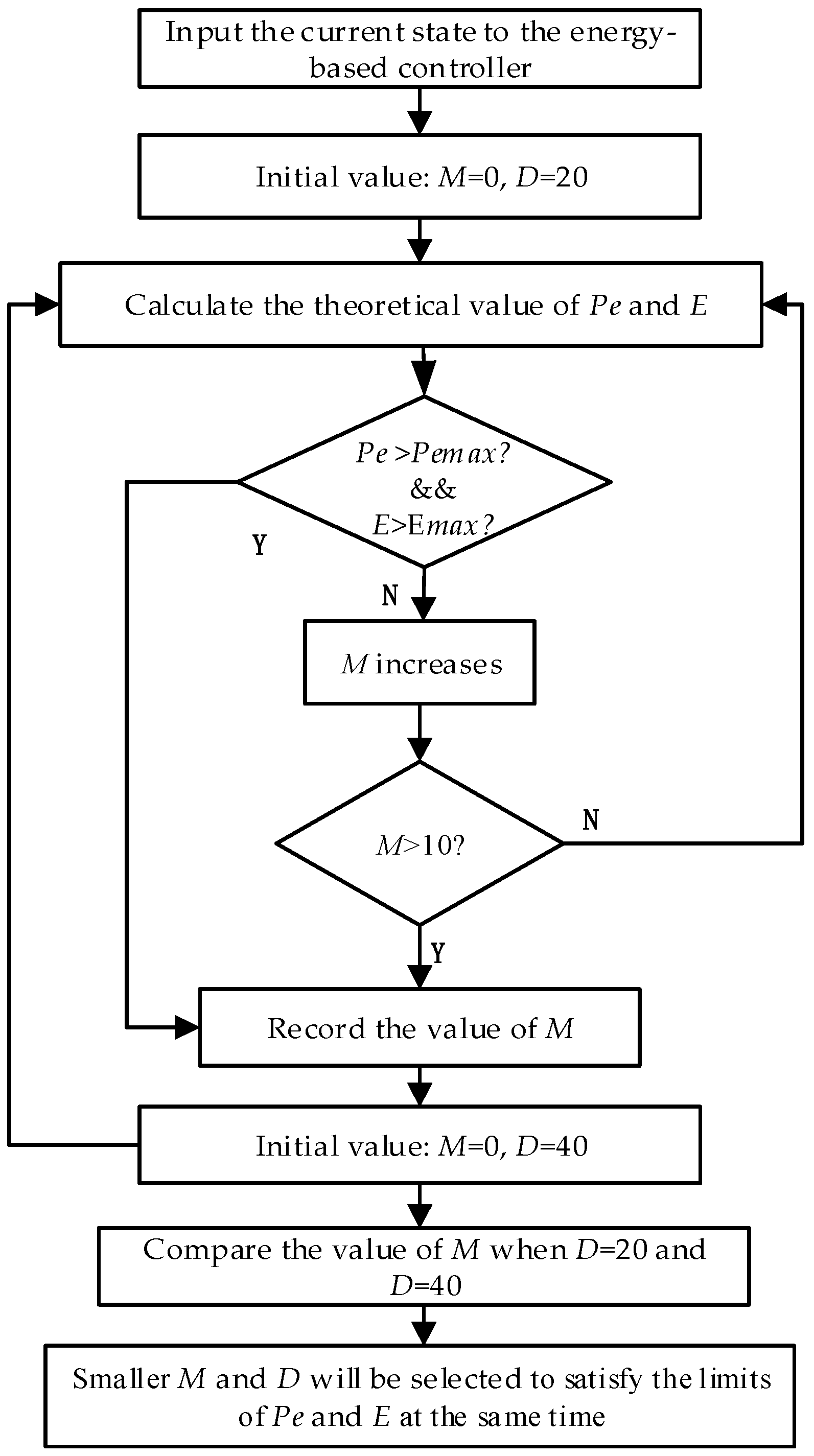
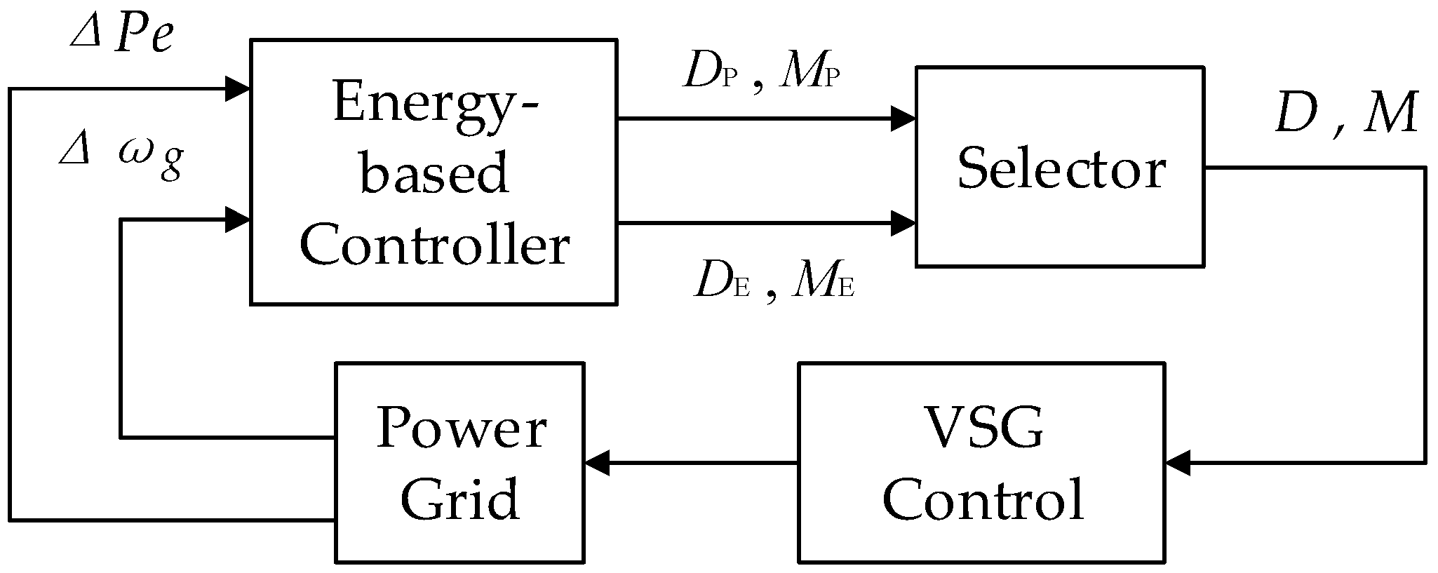
3.3. Design of the Energy Controller with the Restriction of Storage Capacity

As mentioned at the beginning of Section 3, objective formulations are given as Equation (28).

$$\{\begin{array}{ll}{P}_{k.\min }\le \Delta P_e\le P_{k.\max }& (a)\\ E_{k.\min }\le \Delta E\le E_{k.\max }& (b)\end{array},$$

(28)

where P_k.min = 0.8 p.u., P_k.max = 1.2 p.u. (±20% variation from the steady state P_e, 1.0 p.u.) and $\mathsf{∆}$P_e is the output active power. E_k.min is the minimum, E_k.max the maximum and $\mathsf{∆}$E the output energy. E_k.min and E_k.max will not be assigned and the reasons are illustrated in the following analysis.

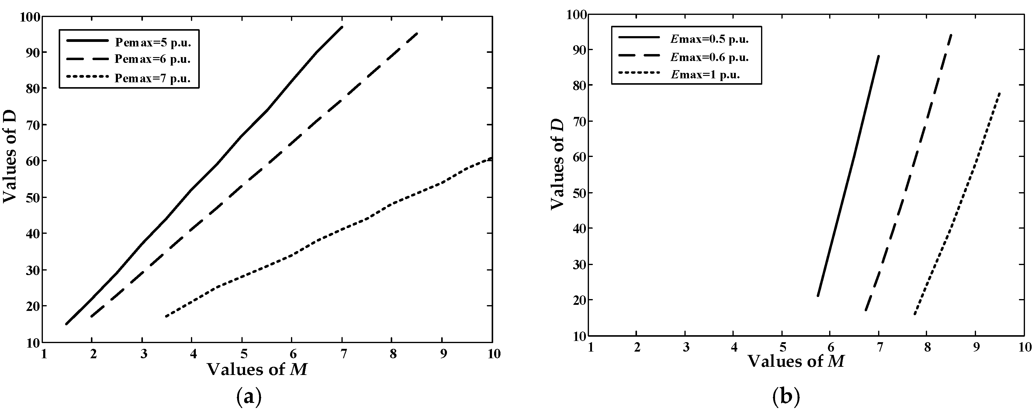
3.3.1. Relations between Storage Capacity Limits and VSG Coefficients

The step response curve of Equation (23) is figured in the condition of underdamping and overdamping, where S₁, S₂, …, S₅ and S₁’ are the areas enclosed by the curves and axes, representing the energy in Figure 3.

In Figure 3a, S₁ is the largest among all the areas. Either of the response curves reaches their first peak, $\mathsf{∆}P$_e reaches its maximum; the first time response curves reach zero, the energy $\mathsf{∆}E$ (S₁ and S₁’) meet the maximum. Through the analysis, the time power and energy of the storage devices reach their limits can be calculated. Meanwhile, the minimum capacity of the storage devices is convenient to access.

Transfer function in Equation (23) can be given in the form containing poles and zeros as Equation (29).

$$\frac{\Delta P_{\mathrm{e}}}{\Delta {\omega }_{\mathrm{g}}}=-\frac{\left[i{s}^2+(ei-gj)s+if-jh\right]\left(s^2+ks-\frac{1}{M}\right)}{\left(s+k\right)\left(s-x_1\right)\left(s-x_2\right)\left(s-x_3\right)\left(s-x_4\right)}.$$

(29)

For the case of a perturbing with ω_g, an inverse transformation of Laplace combined with residue analysis is applied to Equation (29) to obtain Equation (30). Related elements of k_i (i = 1, 2, …, 6) are presented in the Appendix C.

$$\Delta P_e(t)=-(k_1+k_2{e}^{-kt}+k_3{e}^{x_{1}t}+k_4{e}^{x_{2}t}+k_5{e}^{x_{3}t}+k_6{e}^{x_{4}t})\Delta {\omega }_g.$$

(30)

After taking derivatives of Equation (30),

$$0=-(-k_{2}k{e}^{-kt}+x_1{k}_3{e}^{x_{1}t}+x_2{k}_4{e}^{x_{2}t}+x_3{k}_5{e}^{x_{3}t}+x_5{k}_6{e}^{x_{4}t})\Delta {\omega }_{\mathrm{g}}.$$

(31)

The smallest root of the positive roots in Equation (31) is given as t₁, the time when $\mathsf{∆}P$_e reaches its maximum.

$$\Delta P_{e\max }=\Delta P_e(t_1),$$

(32)

The maximum of $\mathsf{∆}E$ can be calculated in Equation (32).

$$\begin{array}{ll}\Delta E_{\max }& ={\displaystyle {\int }_0^{t_2}\Delta P_e(t)}dt\\ & ={\displaystyle {\int }_0^{t_2}-(k_1+k_2{e}^{-kt}+k_3{e}^{x_{1}t}+k_4{e}^{x_{2}t}+k_5{e}^{x_{3}t}+k_6{e}^{x_{4}t})dt}\Delta {\omega }_g(t)\\ & =-k_1{t}_2+\frac{k_2{e}^{-k{t}_2}}{k}-\frac{k_3{e}^{x_1{t}_2}}{x_1}-\frac{k_4{e}^{x_2{t}_2}}{x_2}-\frac{k_5{e}^{x_3{t}_2}}{x_3}-\frac{k_6{e}^{x_4{t}_2}}{x_4}-\frac{k_2}{k}+\frac{k_3}{x_1}+\frac{k_4}{x_2}+\frac{k_5}{x_3}+\frac{k_6}{x_4}\end{array},$$

(33)

where t₂ represents the time when $\mathsf{∆}P$_e becomes 0.00 the first time in underdamping condition, or the time when $\mathsf{∆}P$_e reaches ±0.05 in overdamping condition ($\mathsf{∆}P$_e will infinitely approach zero in overdamping condition and the precision of energy deviation is set as ±0.05 for approximate calculation). It is noticeable that t₂ is generally regarded as a very short period when faults occur and, therefore, $\mathsf{∆}E$ is small and formulations in (b) of Equation (28) can be generally satisfied, explaining the reasons that E_k.min and E_k.max without assignment.

Combined with the Appendix B and Appendix C, both $\mathsf{∆}P$_emax and $\mathsf{∆}E$_max are related to M and D and therefore, detailed studies on their relationship are conducted. In Figure 4, the curves show the influences that M/D exert on $\mathsf{∆}E$_max and $\mathsf{∆}P$_emax while, in Figure 5, the curves show the effect that $\mathsf{∆}E$_max/$\mathsf{∆}P$_emax exert on M and D.

In Figure 4a, relation curves of $\mathsf{∆}E$_max and M, $\mathsf{∆}P$_emax and M are fitted in MATLAB (MATLAB 2012a, MathWorks, USA) when D is constant. When M increases, it is a monotone increasing relationship between $\mathsf{∆}E$_max (or $\mathsf{∆}P$_emax) and M approximately. The bigger the virtual inertia becomes, the larger capacity is needed. In Figure 4b, relation curves of $\mathsf{∆}E$_max and D, $\mathsf{∆}P$_emax and D are fitted when M is constant. When D increases, $\mathsf{∆}E$_max and $\mathsf{∆}P$_emax drop rapidly in a short period, then turn to a mild decrease. Influences that D exert on $\mathsf{∆}E$_max and $\mathsf{∆}P$_emax is smaller than M on $\mathsf{∆}E$_max and $\mathsf{∆}P$_emax.

In Figure 5, it can be concluded that the larger $\mathsf{∆}E$_max and $\mathsf{∆}P$_emax become, the wider the M and D cover. Meanwhile, in any working conditions, relationship between M and D is monotonically when either $\mathsf{∆}E$_max or $\mathsf{∆}P$_emax is constant. Meanwhile, when $\mathsf{∆}E$_max is constant, the variation of M is smaller than those when $\mathsf{∆}P$_emax is constant. In other words, if $\mathsf{∆}P$_e meets the demands in (a) of Equation (28), $\mathsf{∆}E$ follows in (b) of Equation (28) and the illustrations in defining the E_k.min and E_k.max are proved.

3.3.2. Adaptive Control via Energy-Based Algorithms

The energy-based algorithm should work within the restrictions in Equations (27) and (28). The diagram with an additional energy-based control algorithm is shown in Figure 6.

In Figure 6, M_E is the virtual inertia when D = D_E = 20 and M_P the virtual inertia when D = D_P = 40.

According to Equation (27), a detailed algorithm is given in Figure 7.

It is noticeable that the value of D is fixed at 20 or 40, the minimum and maximum of its boundaries. The simplification is reasonable for the influences that D exert on $\mathsf{∆}E$_max and $\mathsf{∆}P$_emax is smaller than that M on $\mathsf{∆}E$_max and $\mathsf{∆}P$_emax, proved in Section 3.3.1. When (M_E, D_E) and (M_P, D_P) are calculated, the smaller one of M_E and M_P will be selected and, therefore, $\mathsf{∆}E$_max and $\mathsf{∆}P$_emax, energy and power needed in suppressing oscillations, is smaller. The effeteness of the algorithm will be proved in Section 4.3.

4. Simulations

Simulations based on VSG of single-machine infinite system were performed on the model in DIgSILENT (DIgSILENT/Power Factory 15.1.7, Germany) of Figure 8 with the parameters of f_base = 50 Hz, P_emax = 0.6 MW, E = 0.3 MW·s, both of which are abstracted from the photovoltaic power plant equipped with storage devices in Qinghai Province, and the renewable energy power was replaced by the DC source. In the simulation, a single lumped model, the replacement of the photovoltaic power plant composed of 34 sets of solar subsystem of the Tucson Power Company, USA is adopted for simplification. Related parameters of the VSG control system and the photovoltaic power station are presented in the

Table A1. Main parameters of Tucson Company Photovoltaic Power Station.

Name	Parameters
Number of solar-cell arrays	34
DC power	4590 kW
AC power	3812 kW
Inverter model	Xantrex PV-150
Number of inverter	34
Rated capacity of inverters	157 kVA
Number of transformers	11
Rated power of transformers	500 kVA
Turns ratio	480 V/34.5 kV

of Appendix D.

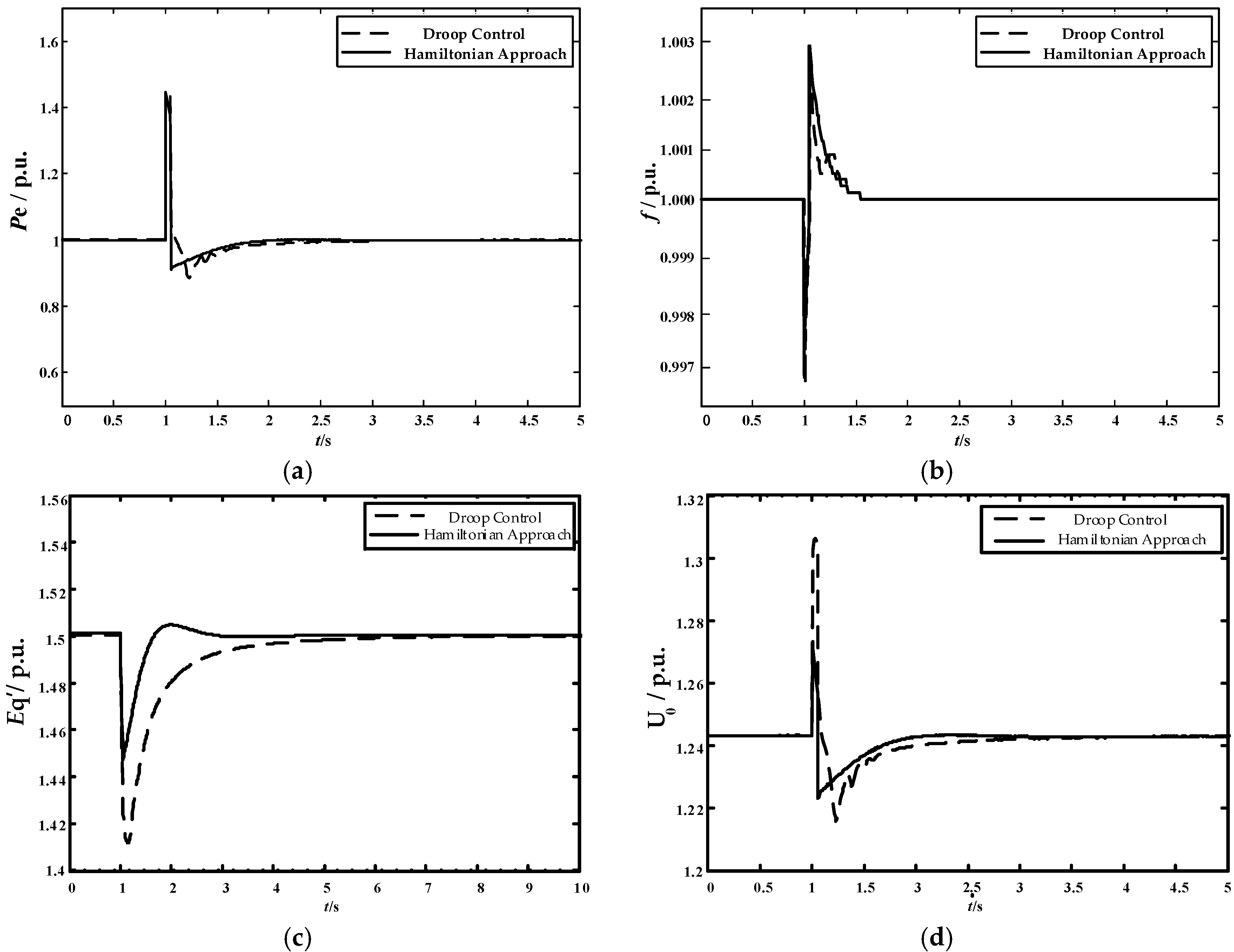
4.1. Comparisons between VSG Based on Droop Control and Hamilton Approach

To verify the superiority of Hamiltonian approach, comparisons are made between different VSG control algorithms—the droop control [10] and the Hamiltonian approach. A three-phase metallic short-circuit fault is set at the middle of the transmission line 3–4 at t = 1 s and the fault is cleared at t = 1.05 s. In Figure 9, responding curves of the output active power P_e, grid frequency f, transient E.M.F E_q’ and output voltage U₀ during fault period are shown in Figure 9a–d.

In these figures, solid curves represent the output of VSG with Hamilton approach while the dotted curves represents the output of VSG with droop control. It is obvious that the advanced algorithm enjoys the enhancement in suppressing oscillations, contributing inertia and shortening the fluctuation period compared to the VSG based on droop control. Validity can be proved that system stability and robustness are strengthened via the VSG based on a Hamilton approach.

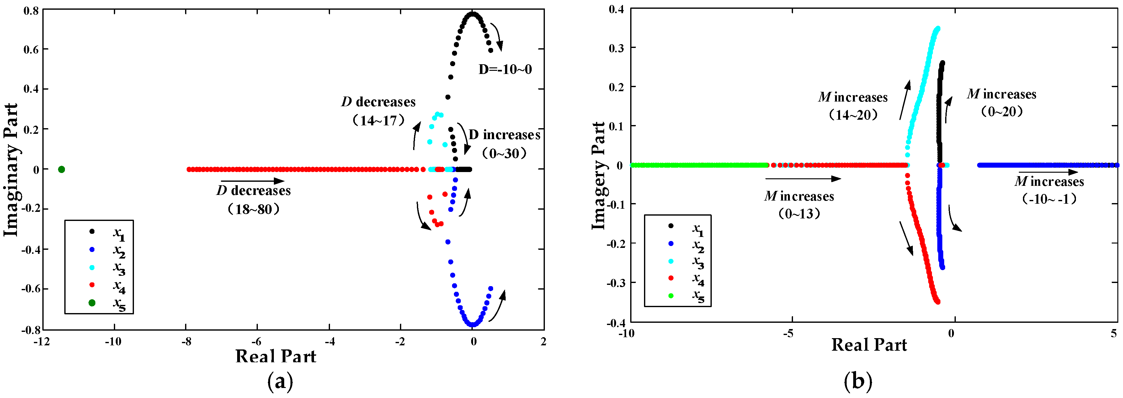
4.2. Effects of Different Controller Coefficients on the System Output Responses

To verify the correctness of the controller coefficient boundaries in Section 3.2, simulations are conducted at the same short-circuit condition above. Output responding curves are presented under different coefficients including M, the virtual inertia and D, the system damping.

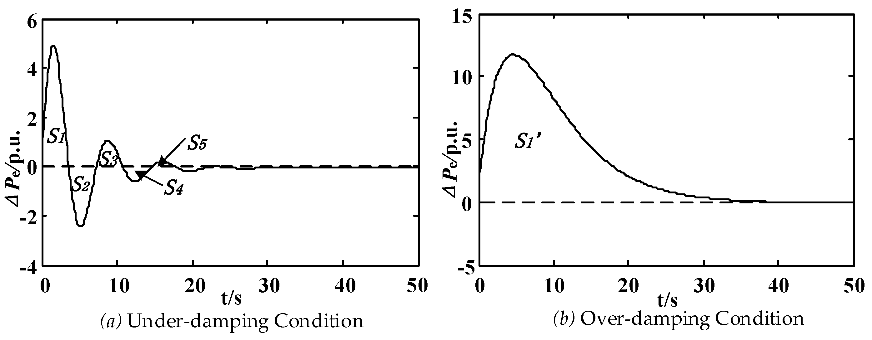
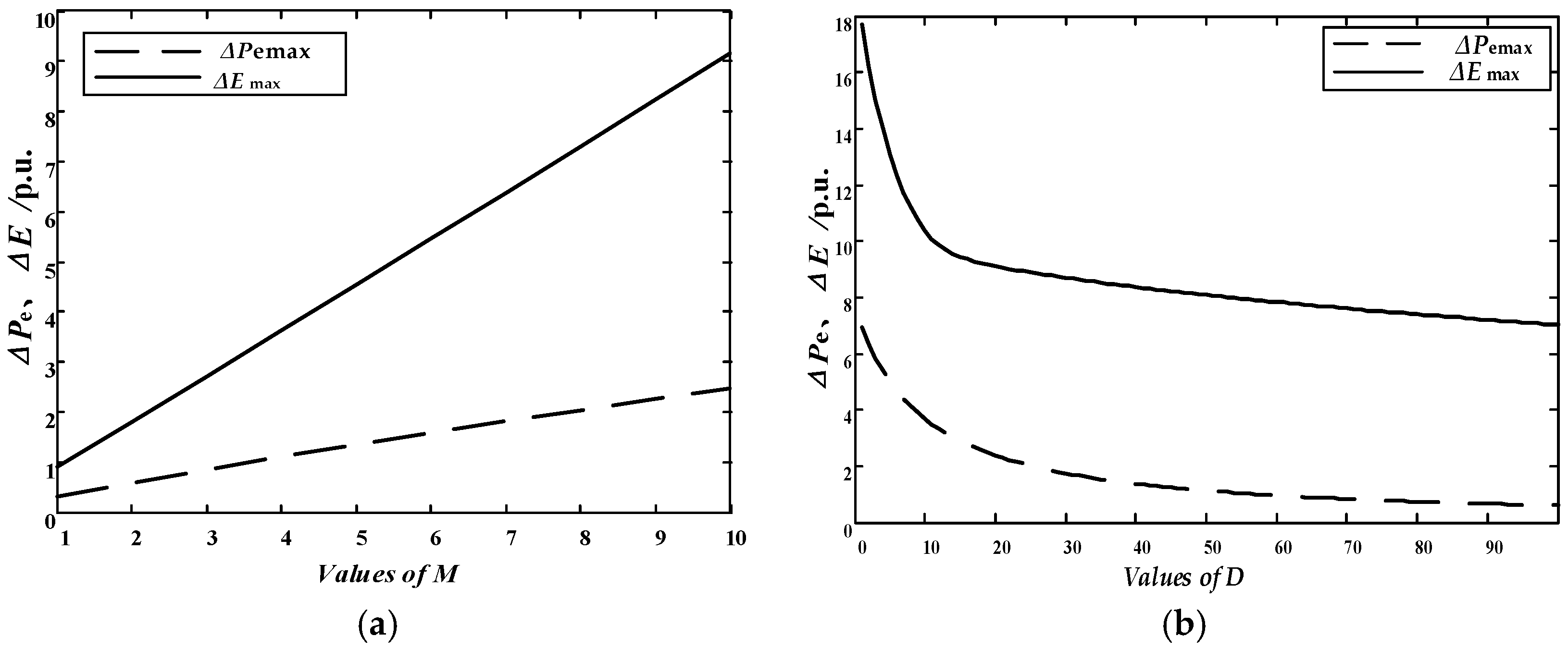
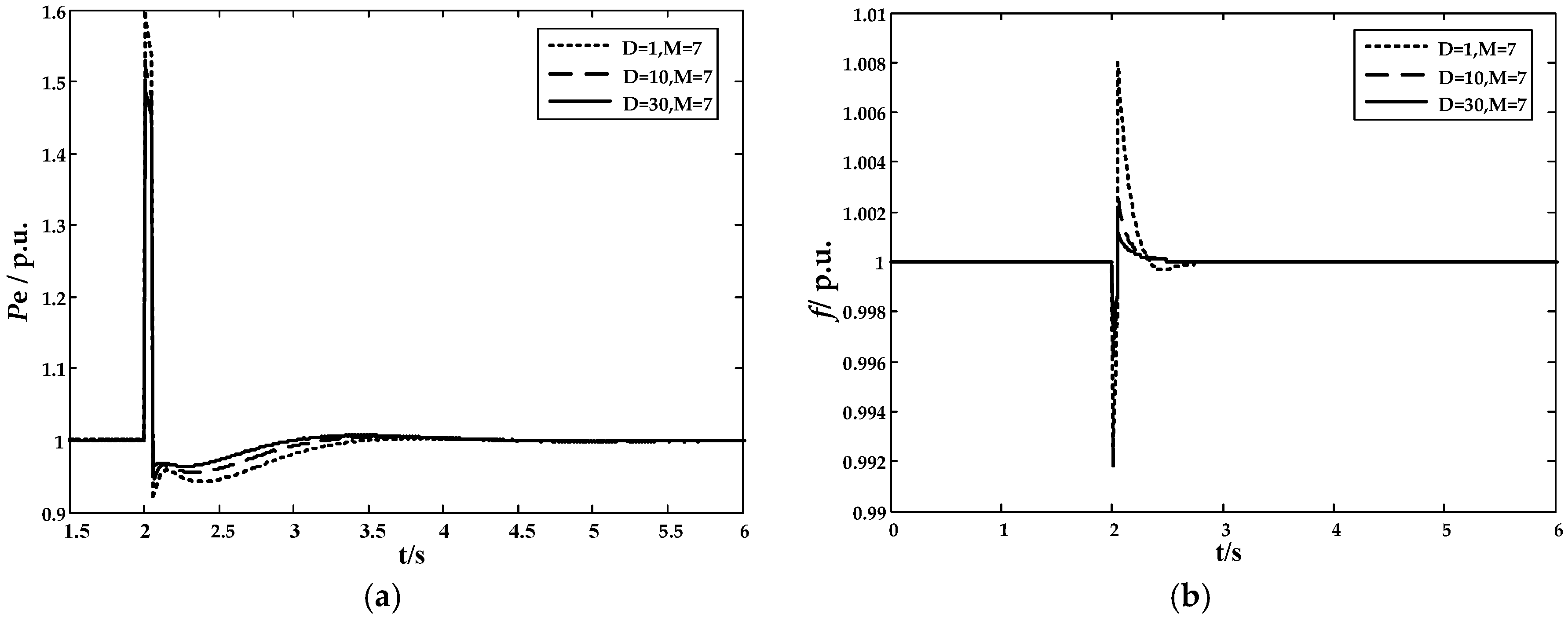
4.2.1. Output Responses with Different D (Virtual Damping)

In this simulation, M is fixed as 7 while D varies from 1 to 30. Curves are shown in Figure 10a,b.

As we can see in Figure 10, it is remarkable in suppress oscillations with a stronger D. When D = 1, it is too weak to suppress system oscillations compared to D = 10. When D = 30, it can be found that an excessive damping constant results in a slower response speed compared to D = 10.

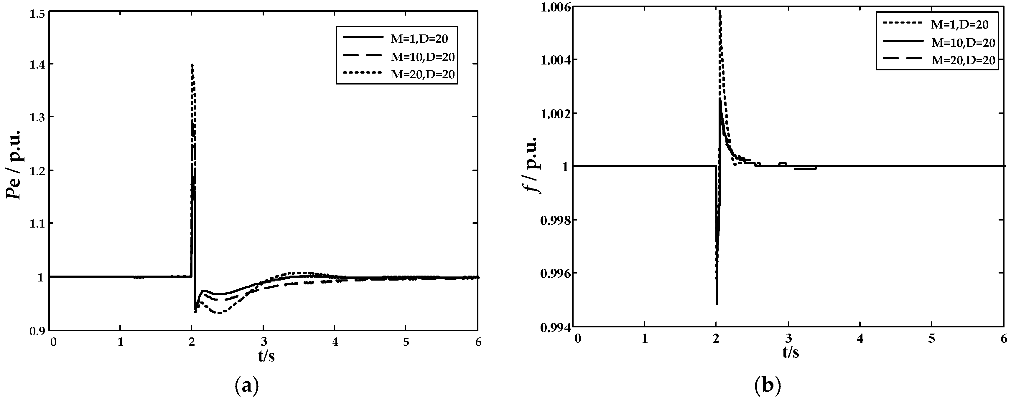
4.2.2. Output Responses with Different M (Virtual Inertia)

In this simulation, D is fixed as 20 while M varies from 1 to 20. Curves are shown in Figure 11a,b.

When M = 1, it is too small for the inertia to suppress the oscillations. When M = 30, the system tends to be in underdamping condition with a long oscillating period for a small damping ratio.

Without taking the limits of the storage capacity into consideration, M varies from 0 to 10 while D from 20 to 40 according to Section 3. The results in Figure 10 verify the boundaries of M and D discussed above, while laying a foundation for a further study.

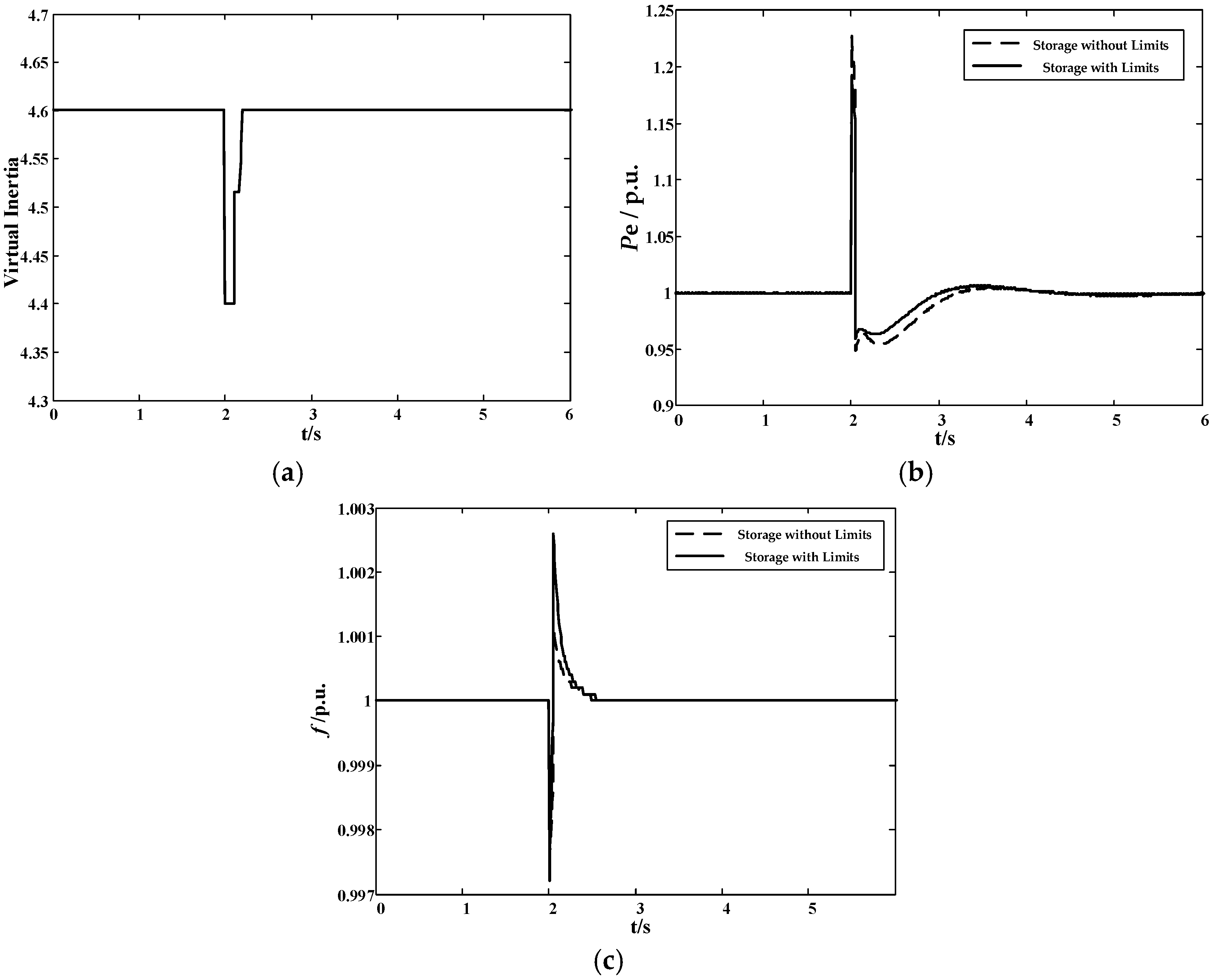
4.3. Comparison between VSG Equipped with Capacity-Limited and Limit-Free Storage Devices

Under the same simulation conditions as above, the variation of M is shown in Figure 12a.

Meanwhile, response curves of output active power P_e and grid frequency f under the storage capacity limits displayed in Figure 12b,c. In those figures, solid curves represent the output of VSG with capacity-limit storage devices while the dotted curves represents the output of VSG with limit-free storage devices.

As can be seen in Figure 12a, during the fault period, the adaptive control of VSG takes effect for keeping the system output to stay within the limits. M drops to 4.4 during the fault and returns to the initial value (M = 4.6) when the fault is cleared. It is noticeable that the variation of D is too small to be recorded. Hence, the variation of D will not be given in figures.

In Figure 12b,c, results are expected that VSG with limit-free storage devices performs better in suppressing oscillations and shortening response time than the one with capacity-limit devices. However, with the advanced algorithm, the virtual inertia of the VSG proposed in the paper is adaptive, falls to 4.4 for the limitation in storage capacity during the transient period. As a result, either $\mathsf{∆}E$_max or $\mathsf{∆}P$_emax becomes smaller and less power is needed to contribute from the storage devices. Meanwhile, although the inertia becomes a smaller value, the VSG system can still keep stabilized and the differences from the counterpart is acceptable. In a word, the results prove the validity and effeteness of the adaptive VSG control algorithm and the energy-based control algorithm.

5. Conclusions

In this paper, an improved VSG model was put forward to enhance system suitability and robustness. A corresponding strategy based on Hamilton theory was then applied to meet the complexity of the model. Compared to the VSG based on droop control via simulations, the advanced model performed better in suppressing oscillations, contributing inertia and shortening the fluctuation period. Boundaries of virtual inertia and damping corresponding to the system stable region were deducted by the study on the small-signal model of VSG. Simulations on the effects that coefficients variation exert on system output responses proved the correctness of the boundaries. To develop the control algorithm with the limits in storage capacity, relations between VSG parameters and charge and discharge capacity were analyzed. The dynamic response of the virtual inertia showed that the proposed VSG made an adaption to satisfy the capacity restriction. With the acceptable cost of losing part of the ability in suppressing oscillations during fault period, the simulations based on improved model worked in the condition closer to the one in practical engineering.

References

1. Mehrasa, M.; Godina, R.; Pouresmaeil, E.; Vechiu, I.; Rodriguez, R.L.; Catalao, J.P.S. Synchronous active proportional resonant-based control technique for high penetration of distributed generation units into power grids. In Proceedings of the IEEE PES Innovative Smart Grid Technologies Conference Europe, Torino, Italy, 26–29 September 2017; IEEE: Piscataway, NJ, USA, 2017; pp. 1–6. [Google Scholar]
2. Pouresmaeil, E.; Mehrasa, M.; Godina, R.; Vechiu, I.; Rodriguez, R.L.; Catalao, J.P.S. Double synchronous controller for integration of large-scale renewable energy sources into a low-inertia power grid. In Proceedings of the IEEE PES Innovative Smart Grid Technologies Conference Europe, Torino, Italy, 26–29 September 2017; IEEE: Piscataway, NJ, USA, 2017; pp. 1–6. [Google Scholar]
3. Mehrasa, M.; Adabi, M.E.; Pouresmaeil, E.; Adabi, J.; Bo, N.J. Direct Lyapunov control (DLC) technique for distributed generation (DG) technology. Electr. Eng. 2014, 96, 309–321. [Google Scholar] [CrossRef]
4. Mehrasa, M.; Rezanejhad, M.; Pouresmaeil, E.; Catalão, J.P.S.; Zabihi, S. Analysis and control of single-phase converters for integration of small-scaled renewable energy sources into the power grid. In Proceedings of the Power Electronics and Drive Systems Technologies Conference, Tehran, Iran, 16–18 February 2016; IEEE: Piscataway, NJ, USA, 2016; pp. 384–389. [Google Scholar]
5. Beck, H.P.; Hesse, R. Virtual synchronous machine. In Proceedings of the International Conference on Electrical Power Quality and Utilization, Barcelona, Spain, 9–11 October 2007; IEEE: Piscataway, NJ, USA, 2007; pp. 1–6. [Google Scholar]
6. Zhong, Q.C.; Weiss, G. Synchronverters: Inverters that mimic synchronous generators. IEEE Trans. Ind. Electron. 2011, 58, 1259–1267. [Google Scholar] [CrossRef]
7. Loix, T.; Breucker, S.D.; Vanassche, P.; Keybus, J.V.D.; Driesen, J.; Visscher, K. Layout and performance of the power electronic converter platform for the VSYNC project. In Proceedings of the IEEE Bucharest PowerTech, Bucharest, Romania, 28 June–2 July 2009; IEEE: Piscataway, NJ, USA, 2009; pp. 1–8. [Google Scholar]
8. Chen, Y.; Hesse, R.; Turschner, D.; Beck, H.P. Comparison of methods for implementing virtual synchronous machine on inverters. In Proceedings of the International Conference on Renewable Energies and Power Quality, Santiago de Compostela, Spain, 28–30 March 2012; p. 6. [Google Scholar]
9. Liu, J.; Miura, Y.; Ise, T. Dynamic characteristics and stability comparisons between virtual synchronous generator and droop control in inverter-based distributed generators. IEEE Trans. Power Electron. 2014, 31, 1536–1543. [Google Scholar]
10. D’Arco, S.; Suul, J.A.; Fosso, O.B. Small-signal modelling and parametric sensitivity of a Virtual Synchronous Machine. In Proceedings of the Power Systems Computation Conference, Wroclaw, Poland, 18–22 August 2014; IEEE: Piscataway, NJ, USA, 2014; pp. 1–9. [Google Scholar]
11. Karapanos, V.; Kotsampopoulos, P.; Hatziargyriou, N. Performance of the linear and binary algorithm of virtual synchronous generators for the emulation of rotational inertia. Electr. Power Syst. Res. 2015, 123, 119–127. [Google Scholar] [CrossRef]
12. Alipoor, J.; Miura, Y.; Ise, T. Power system stabilization using virtual synchronous generator with alternating moment of inertia. IEEE J. Emerg. Sel. Top. Power Electron. 2015, 3, 451–458. [Google Scholar] [CrossRef]
13. Alipoor, J.; Miura, Y.; Ise, T. Distributed generation grid integration using virtual synchronous generator with adoptive virtual inertia. In Proceedings of the Energy Conversion Congress and Exposition, Denver, CO, USA, 15–19 September 2013; IEEE: Piscataway, NJ, USA, 2013; Volume 8237, pp. 4546–4552. [Google Scholar]
14. Chong, C.; Yang, H.; Zheng, Z.; Tang, S.; Zhao, R. Rotor inertia adaptive control method of VSG. Autom. Electr. Power Syst. 2015, 39, 82–89. [Google Scholar]
15. Miguel, A.T.L.; Lopes, L.A.C.; Luis, A.M.T.; José, R.E.C. Self-tuning virtual synchronous machine: A control strategy for energy storage systems to support dynamic frequency control. IEEE Trans. Energy Convers. 2014, 29, 833–840. [Google Scholar]
16. Wang, Y.; Cheng, D.; Liu, Y.; Li, C. Adaptive H∞ excitation control of multi-machine power systems via the Hamiltonian function method. Int. J. Control 2004, 77, 336–350. [Google Scholar] [CrossRef]
17. Xi, Z.; Cheng, D.; Lu, Q.; Mei, S. Nonlinear decentralized controller design for multi-machine power systems using Hamiltonian function method. Automatica 2002, 38, 527–534. [Google Scholar] [CrossRef]
18. Galaz, M.; Ortega, R.; Bazanella, A.S.; Stankovic, A.M. An energy-shaping approach to the design of excitation control of synchronous generators. Automatica 2003, 39, 111–119. [Google Scholar] [CrossRef]
19. Wang, Y.; Cheng, D.; Hong, Y. Stabilization of synchronous generators with the Hamiltonian function approach. Int. J. Syst. Sci. 2001, 32, 971–978. [Google Scholar] [CrossRef]
20. Qian, J.; Zeng, Y.; Zhang, L.; Xu, T. Hamiltonian modeling of generator integrated AVR and PSS. Procedia Eng. 2012, 31, 1217–1224. [Google Scholar] [CrossRef]
21. Castro, G.; Bermúdez, J.; Jiménez, M.; Alvarez, M.; Arreaza, A. AVRs and PSSs revisited. In Proceedings of the International Conference on Electrical and Electronics Engineering, Bursa, Turkey, 26–28 November 2015; IEEE: Piscataway, NJ, USA, 2016; pp. 1006–1010. [Google Scholar]
22. Bevrani, H.; Ise, T.; Miura, Y. Virtual synchronous generators: a survey and new perspectives. Int. J. Electr. Power Energy Syst. 2014, 54, 244–254. [Google Scholar] [CrossRef]
23. Wesenbeeck, M.P.N.V.; Haan, S.W.H.D.; Varela, P.; Visscher, K. Grid tied converter with virtual kinetic storage. In Proceedings of the IEEE Bucharest PowerTech, Bucharest, Romania, 28 June–2 July 2009; IEEE: Piscataway, NJ, USA, 2009; pp. 1–7. [Google Scholar]
24. Albu, M.; Visscher, K.; Creanga, D.; Nechifor, A.; Golovanov, N. Storage selection for DG applications containing virtual synchronous generators. In Proceedings of the IEEE Bucharest PowerTech, Bucharest, Romania, 28 June–2 July 2009; IEEE: Piscataway, NJ, USA, 2009; pp. 1–6. [Google Scholar]
25. Vassilakis, A.; Kotsampopoulos, P.; Hatziargyriou, N.; Karapanos, V. A battery energy storage based virtual synchronous generator. In Proceedings of the IREP Symposium Bulk Power System Dynamics and Control—IX Optimization, Security and Control of the Emerging Power Grid, Rethymno, Greece, 25–30 August 2013; IEEE: Piscataway, NJ, USA, 2013; pp. 1–6. [Google Scholar]
26. Benidris, M.; Elsaiah, S.; Sulaeman, S.; Mitra, J. Transient stability of distributed generators in the presence of energy storage devices. In Proceedings of the North American Power Symposium, Champaign, IL, USA, 9–11 September 2012; IEEE: Piscataway, NJ, USA, 2012; pp. 1–6. [Google Scholar]
27. D’Arco, S.; Suul, J.A. Virtual synchronous machines—Classification of implementations and analysis of equivalence to droop controllers for microgrids. In Proceedings of the Powertech, Grenoble, France, 16–20 June 2013; IEEE: Piscataway, NJ, USA, 2013; pp. 1–7. [Google Scholar]
28. Ma, Y.; Yu, R.; Liu, H.; Zhao, S. The analysis of VSG control algorithm base on Hamiltonian system. Power Syst. Technol. 2017, 41, 2543–2553. [Google Scholar]
29. Maschke, B.; Ortega, R.; van der Schaft, A.J. Energy-based Lyapunov functions for forced Hamiltonian systems with dissipation. IEEE Trans. Autom. Control 2000, 45, 1498–1502. [Google Scholar] [CrossRef]
Figure 1. Block diagram of the VSG control strategy.
Energies 11 00677 g001
Figure 2. Roots of the poles with the variations of the parameters. (a) Pole Loci when M a constant value; (b) Pole Loci when D a constant value.
Energies 11 00677 g002
Figure 3. Step response with different damping ratio. (a) Active power response in under-damping condition (b) Active power response in over-damping condition.
Energies 11 00677 g003
Figure 4. Relationship between the Capacity limits of the energy storage equipment and the parameters. (a) Storage capacity limits with M; (b) Storage capacity limits with D.
Energies 11 00677 g004
Figure 5. Relation of M and D under different storage limits. (a) Relation of M and D when P emax = Const; (b) Relation of M and D when E max = Const.
Energies 11 00677 g005
Figure 6. Energy-based control algorithm.
Energies 11 00677 g006
Figure 7. Energy control algorithm process.
Energies 11 00677 g007
Figure 8. The simulation system diagram.
Energies 11 00677 g008
Figure 9. System outputs during short-circuit fault period. (a) Output active power Pe/p.u.; (b) Grid frequency f/p.u.; (c) Transient E.M.F Eq’/p.u.; (d) Output voltage U0/p.u.
Energies 11 00677 g009
Figure 10. Output responses with different damping under short-circuit fault condition. (a) Comparisons of Pe/p.u.; (b) Comparisons of f/p.u.
Energies 11 00677 g010
Figure 11. Output responses with different virtual inertia under short-circuit fault condition. (a) Comparisons of Pe/p.u.; (b) Comparisons of f/p.u.
Energies 11 00677 g011
Figure 12. Figures of system output with limited/limit-free energy storage capacity. (a) Variation of the virtual inertia; (b) Comparison of Pe/p.u; (c) Comparison of f/p.u.
Energies 11 00677 g012