Optimizing Energy Storage Capacity in Islanded Microgrids Using Immunity-Based Multiobjective Planning

Abstract

Microgrid operation is challenging because the amount of electricity that is produced from renewables is uncertain and the inertia of distributed generation resources is very small. Energy storage systems can regulate energy, improve the reliability of the power system and enhance the transient stability. This paper determines the optimal capacities of energy storage systems in an islanded microgrid that is composed of wind-turbine generators, photovoltaic arrays, and micro-turbine generators. The energy storage system can enhance the reliability of the microgrid and eliminate the unnecessary load shedding when a severe transient (such as a generator outage) occurs in the islanded microgrid. The studied problem is expressed as a multi-objective programming formulation, which is solved using an immunity-based algorithm. Four objective functions are optimized: minimum of energy storage capacity, minimum of load shedding, maximum of the lowest swing frequency, and minimum of the Customer Average Interruption Duration Index (CAIDI). These four objective functions are subject to both steady-state constraints and the transient-state equality constraint. The steady-state constraints include the total shed load limit, the feasible range of energy storage capacities while the transient-state equality constraint is expressed by the dynamic equation. The Pareto optimums are explored and optimality of the problem is investigated. The simulation results based on an islanded 15-bus microgrid show the applicability of the proposed method.

1. Introduction

The establishment of microgrids is an efficient approach to accommodate distributed generation (DG) resources and increase the penetration of DG in the main power grid [1,2]. Microgrids generally include devices for generating energy from renewable sources (such as wind and photovoltaic power), small generation units (such as diesel and microturbine generators) and energy storage systems [3,4]. Many works have sought to develop the microgrid test bed. Consortium for Electric Reliability Technology Solutions (CERTS) microgrid concepts were first formulated in 1998 [1], and Lasseter subsequently published an evaluation report for this test bed [2]. Lasseter presented some crucial concepts concerning the CERTS microgrid test bed, such as embedding peer-to-peer and plug-and-play devices in the microgrid.

In a microgrid, power generation resources may include renewable energy and micro-turbine generators, while the battery energy storage system (BESS) enables bidirectional energy flow [5]. The amount of electrical power generated from renewable sources of energy is uncertain because of their intermittence [6]. The microturbine generator has a high-speed single-shaft design, in which the compressor and turbine are mounted on the same shaft as the permanent magnet synchronous generator [7]. The microturbine generator can combine heat and provide electricity stably to local customers in microgrids [8]. The BESS provides voltage support [9] and regulates system frequency [10,11]. The BESS can be also used to mitigate fluctuations of the output power from PV arrays and wind farms [12]. Sometimes, the BESS may incorporate a diesel or micro-turbine generator to filter the oscillating output power from renewables [13,14] and provide a seamless transition between standalone and grid-tied modes [15].

The size of the BESS should be determined in the planning stage by considering different factors. Gitizadeh and Fakharzadegan [16] considered the adoption of time-of-use pricing using mixed integer programming to implement load shifting and peak shaving. Maleki and Askarzadeh [17] used a discrete version of harmony search to determine the number of PV panels, wind turbines, and batteries, which store excess energy for later use under deficit conditions. Ma et al. [18] utilized the Hybrid Optimization Model for Electric Renewable (HOMER) software to study thousands of cases to determine an optimal autonomous system configuration in terms of system net present cost (NPC) and cost of energy (COE); the effects of the size of the PV panels, the size of the wind turbines and the capacity of the battery bank on economic performance of the system were examined [19]. Ekren [20] used a simulated annealing algorithm to determine the PV size, area swept by wind turbine rotors and battery capacity that minimized the total cost of a hybrid energy system. Ekren [21] optimized the size of a PV/wind integrated hybrid energy system with battery storage under various loads and the unit cost of auxiliary energy sources using the commercial software, OptQuest; the results of the optimization were confirmed using Loss of Load Probability (LOLP) and autonomy analysis. Mohammadi [22] proposed a two-stage scenario-based programming model, whose first stage prescribed the here-and-now variables (i.e., binary variables for the statuses of generation units) and whose second stage optimized the values of the wait-and-see variables (i.e., continuous variables for the amounts of power generations) under cost minimization, with the purpose of determining the size of the BESS to accumulate energy when production exceeded demand to make it available at the request of the users. Quevedo and Contreras [23] explored the best locations of both BESS by optimizing distribution system costs taking into account network constraints. Han et al. [24] proposed a method to minimize the total power capacity of candidate energy storage facilities when the availability of existing flexible resources is maximized.

This paper proposes a novel method for determining the capacity of the BESS in an islanded microgrid, considering both steady-state and dynamic constraints. The BESS (1) improves reliability [25,26]; (2) stabilizes transients [27]; and (3) reduces load shedding [28]. The studied problem herein is expressed as a multi-objective optimization that involves the dynamic equations of the power system. The dynamic equations are related to the transients that are caused by an outage of a large micro-turbine generator. When the large micro-turbine generator outage occurs, partial loads are shed by underfrequency relays to prevent blackout. The decision variables are the numbers of batteries at different candidate buses and the amounts of the loads shed in different stages of the under-frequency relays [28]. An immunity-based algorithm, called the Chaos Clonal Evolutionary Algorithm [29], is utilized to optimize the four objectives to gain the Pareto optimums. The contributions of this paper are summarized as follows:

(a)

The proposed method considers both steady-state and dynamic constraints in the multiobjective optimization; however, existing methods only considered steady-state constraints when BESS planning was considered [16,17,18,19,20,21,22,23,24]. Time-domain transient-state constraints are considered in the proposed method to set the underfrequency relays. A co-simulation method is implemented in this paper.

(b)

Traditional methods only addressed the cost of BESS rather than reliability in the bulk power system/microgrid expect for [22,23]. Instead of whole system indices adopted in [22,23], this work considers a reliability index at a specific customer.

(c)

Four objective functions are optimized: minimum of energy storage capacity, minimum of load shedding, maximum of the lowest swing frequency, and minimum of the Customer Average Interruption Duration Index (CAIDI). The Pareto optimums are explored and optimality of the problem is investigated.

(d)

Comparative studies verify that the optimal solution obtained by the proposed immunity-based algorithm is better than that by the traditional genetic algorithms (GA).

The rest of the paper is organized as follows: Section 2 presents a detailed description and formulation of the problem. Section 3 presents the proposed method, which involves chaos clonal evolutionary programming. Section 4 presents the results of simulations that concern the Pareto frontier. Section 5 draws conclusions.

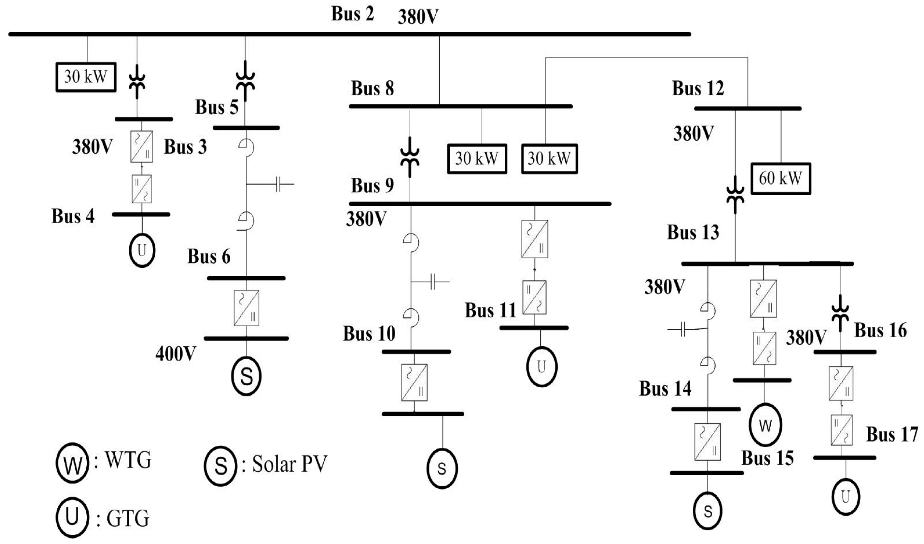
2. Problem Description, Modeling and Formulation

At the planning stage, the new BESS is used to enhance the reliability of a power system and provides energy to maintain the system frequency in case of an emergency. The reliability is related to the steady-state condition and the variation of the system frequency is obtained by solving the aforementioned dynamic equations.

2.1. Reliability

Installation of a new BESS can enhance the reliability of the microgrid. Reliability is a measure of the quality of power supply in an electric power system [30]. Many reliability indices for power systems are used. Since the microgrid supplies electric power from existing renewables and microturbines directly to local customers, the System Average Interruption Frequency Index (SAIFI), the System Average Interruption Duration Index (SAIDI) and the customer average interruption duration index (CAIDI), rather than LOLP, Ref. [31] are discussed herein. SAIFI is the average number of interruptions (occurrence/year) that a customer experiences, and is expressed as:

$$\mathrm{SAIFI}\equiv \frac{\mathrm{total} \mathrm{number} \mathrm{of} \mathrm{customers} \mathrm{of} \mathrm{interruptions}}{\mathrm{total} \mathrm{number} \mathrm{of} \mathrm{customers} \mathrm{served}}\equiv \frac{{{\displaystyle \sum }}^{}{\lambda }_{\zeta }{N}_{\zeta }}{N_T}$$

(1)

where ${\lambda }_{\zeta }, N_{\zeta }$ and N_T are the failure rate (occurrence/year), the number of customers at location $\zeta$, and the total number of customers served, respectively. SAIDI, on the other hand, is the average outage duration (h/year or min/year) for each customer served, and is defined as follows:

$$\mathrm{SAIDI}\equiv \frac{\mathrm{sum} \mathrm{of} \mathrm{all} \mathrm{customer} \mathrm{interruption} \mathrm{durations}}{\mathrm{total} \mathrm{number} \mathrm{of} \mathrm{customers} \mathrm{served}}\equiv \frac{{{\displaystyle \sum }}^{}{u}_{\zeta }{N}_{\zeta }}{N_T}$$

(2)

where $u_{\zeta }$ is the annual outage time (h or min per year) at location $\zeta$. Finally, CAIDI (h or min per occurrence) is defined by:

$$\mathrm{CAIDI}\equiv \frac{\mathrm{SAIDI}}{\mathrm{SAIFI}}=\frac{\mathrm{sum} \mathrm{of} \mathrm{all} \mathrm{customer} \mathrm{interruption} \mathrm{durations}}{\mathrm{total} \mathrm{number} \mathrm{of} \mathrm{customers} \mathrm{of} \mathrm{interruptions}}\equiv \frac{{{\displaystyle \sum }}^{}{u}_{\zeta }{N}_{\zeta }}{{{\displaystyle \sum }}^{}{\lambda }_{\zeta }{N}_{\zeta }}$$

(3)

When new energy systems are considered, their failure rates and annual outage times and number of BESS will have an impact on CAIDI. A smaller CAIDI indicates better reliability.

2.2. Underfrequency Load Shedding

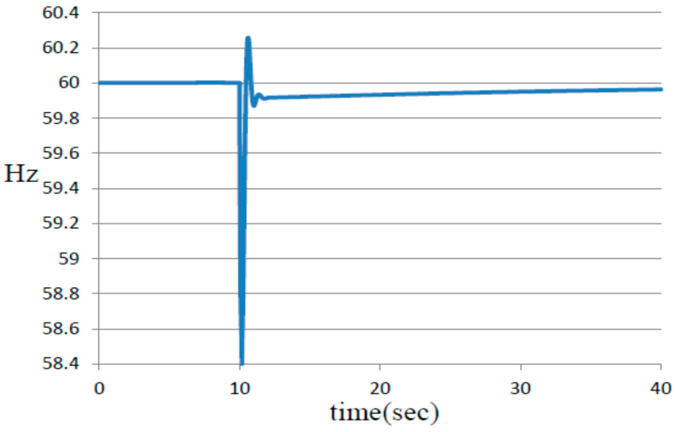
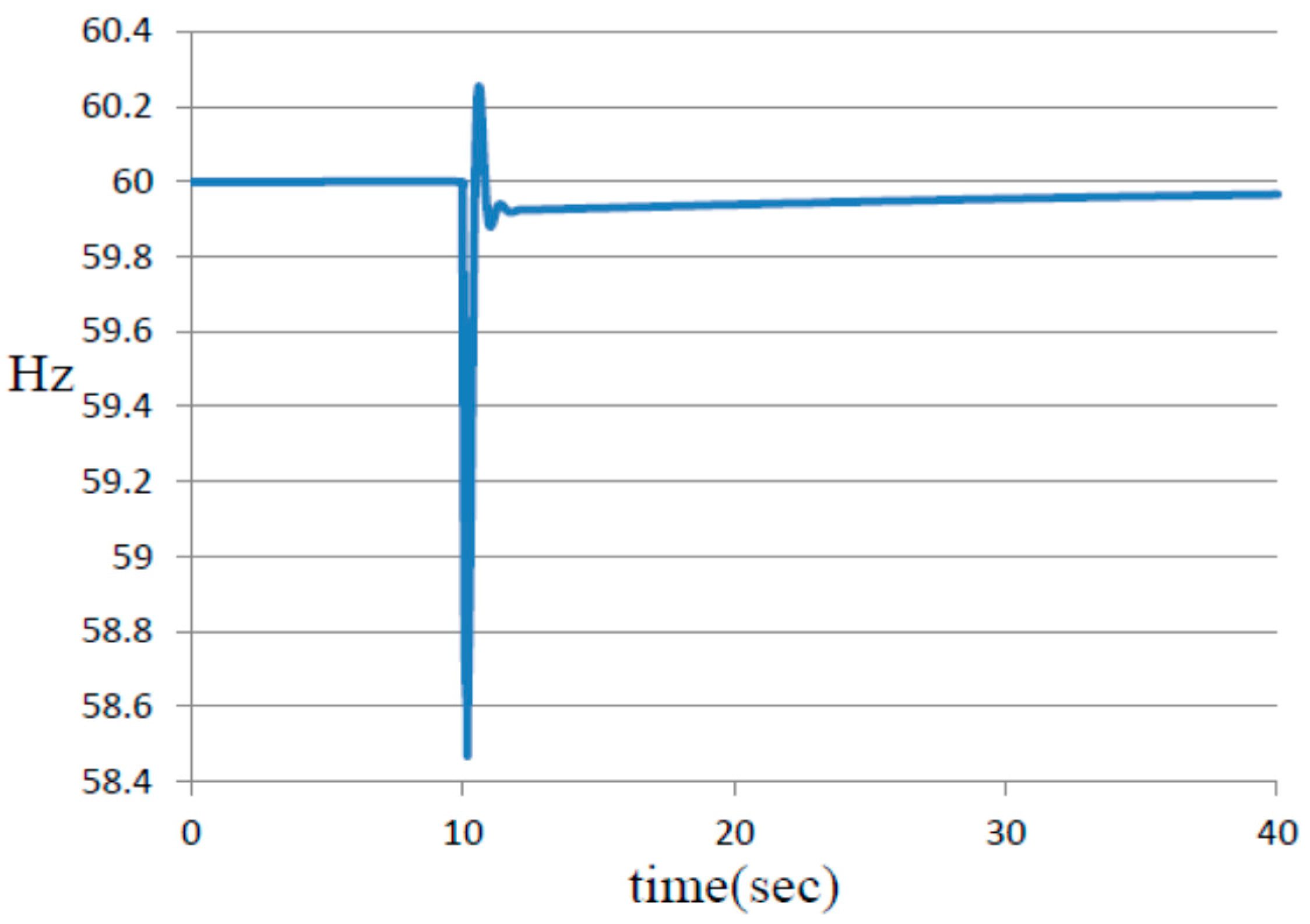
The microgrid should be operated with a nominal frequency of 50 or 60 Hz. When a critical component outage occurs, e.g., a loss of a large micro-turbine generator, the system frequency decreases because the power generation instantaneously drops below demand. If no action (such as partial load shedding) is taken, then the blackout is likely to occur in the microgrid. Thus, the underfrequency relay must be used to shed partial system load to prevent the system from blackout [32].

The parameters of an underfrequency relay are the amount of load shed at specified frequencies, such as 58.8, 58.2, 57.6, …, and 54.6 Hz in eight stages. Since the BESS can provide excess energy to the system loads in an emergency (when the frequency falls), this work determines the capacity of the BESS and each amount of load shed in various stages of underfrequency relays.

The system frequency is calculated by solving both the linearized network equations and the dynamic equations for the microgrid. This will be explained in the next section.

2.3. System Frequency

Dynamic responses of a traditional power system can be expressed by linearized network (power flow) equations and many differential equations for generators that depend on the models of the exciters and the governors [33]. For a microgrid, the distributed generation resources are generally implemented using an inverter-based control [34]. The nonlinear system equations for the microgrid can be linearized around a nominal operating point to yield a set of linearized system equations in matrix form:

$$\dot{\widehat{x}}=A\widehat{x}+b\widehat{u}$$

(4)

$$\widehat{y}=c\widehat{x}$$

(5)

where $\widehat{x}, \widehat{y}$ and $\widehat{u}$ are the state vector, the output vector and the external or compensated input vector and A, b and c are all constant matrices (vectors) of appropriate dimensions. The state vector in Equations (4) and (5) can be partitioned into two substate vectors as $\widehat{x}=[{\widehat{x}}_{DG}$, ${\widehat{x}}_{load}],$ where ${\widehat{x}}_{DG}$ and ${\widehat{x}}_{load}$ are referred to as the system state vectors of the inverter-based distributed generation (DG) and the local load, respectively. One of the elements in $\widehat{y}$ is the system frequency; other elements include line flows and power injections.

Because the system frequency mainly depends on the operation of gas-turbine governor, power converter (inverter), and energy storage system, their models will be detailed in the following subsections. These models are implemented in the software NEPLAN 5.5.0 (NEPLAN AG, Zürich, Switzerland) [35], which computes the system frequency and CAIDI in the co-simulation.

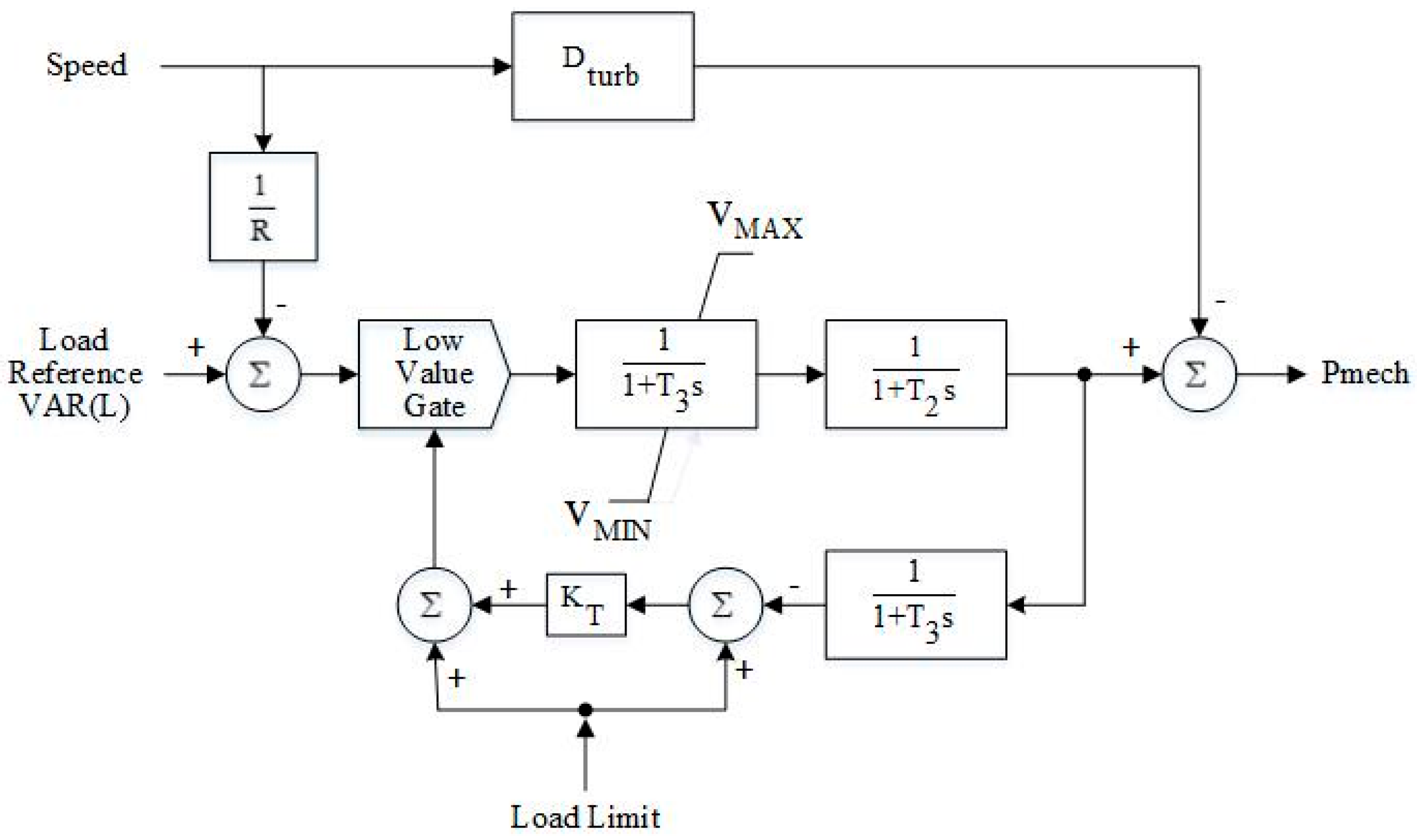
2.4. Gas Turbine Model

The governor of gas turbine has a great impact on the system frequency. The gas turbine consists of a turbine, an axial compressor, and a combustion chamber. The air supporting the combustion process is compressed via the axial compressor. This air is then mingled with fuel in the chamber. Figure 1 illustrates this model comprising droop control and three time constants: T1, T2 and T3 mean the fuel valve response, turbine response, and load limit response, respectively [36].

2.5. Converter

Types of converters include rectifiers and inverters, which can be modeled using the following equations [35]:

$$V_d=V_{do}\times \cos \left(\alpha \right)\times \frac{3}{\pi }\times X_c\times B\times I_d$$

(6)

$$V_{do}=\frac{3\sqrt{2}}{\pi }\times B\times T\times E_{ac}$$

(7)

$$Q_{ac}=P_{ac}\times tan\left(\phi \right)$$

(8)

$$P_{ac}=P_d=V_d{I}_d$$

(9)

$$I_{ac}=\frac{\sqrt{6}B}{\pi }\times V_d{I}_d$$

(10)

$V_d$ and $E_{ac}$ denote the DC and AC voltages of the converter, respectively. $P_{ac}$ and $Q_{ac}$ represent the real and reactive powers at the AC terminal, respectively. $P_d$ is the DC power at the DC terminal. $I_{ac}$ and $I_d$ are the converter AC and DC currents, respectively. B signifies the number of bridges. $X_c$ is the commutating reactance. The symbols $\phi$ and α mean the power factor angle and rectifier firing angle, respectively.

If the rectifier is in its current control mode, a voltage margin of approximate 3% is maintained. If the firing angle is kept within [5°, 7°], then 14° ≤ α ≤ 16°. If the controlled AC voltage of the rectifier is too low, the inverter will be switched to the current control mode.

2.6. Lithium-Ion Model

Lithium-ion batteries are adopted for the energy storage system. Let $V_{bat}$ and $E_o$ be the battery terminal and internal voltages, respectively. The parameter R and variable i are the internal resistance and current, respectively. The discharge and charge modes of this energy storage system can be formulated by Equations (11) and (12) as follows [35]:

$$V_{bat}=E_o-R·i-K\frac{Q}{Q-IT}\left(IT+i_{Lag}\right)+A·exp\left(-D·IT\right)$$

(11)

$$V_{bat}=E_o-R·i-\frac{K·Q·i_{Lag}}{IT+0.1Q}-K\frac{Q}{Q-IT}IT+A·exp\left(-D·IT\right)$$

(12)

where K and Q denote the polarization constant (V/Ah) and capacity (Ah), respectively. Parameters A and D signify the exponential zone amplitude (V) and inverse of exponential zone time constant (1/Ah), respectively. Also, IT = ${{\displaystyle \int }}^{}i\mathrm{dt} \mathrm{and} i_{Lag}=\frac{i}{1+T_{Lag}}.$

2.7. Problem Formulation

Let the variable $\widehat{p}$ be the vector of the shed load in the eight stages, [p₁, p₂, …, p₈]. The variable $\widehat{n}$ represents the vector of the numbers of batteries at all candidate buses, [n₁, n₂, …, n_c, …, n_C], where C is the number of candidate buses for the BESS installation. The variable $n_c$ is the number of batteries at candidate bus c. Let objectives $f_1\left(\widehat{p}, \widehat{n}\right), f_2\left(\widehat{p}, \widehat{n}\right), f_3\left(\widehat{p}, \widehat{n}\right) \mathrm{and} f_4\left(\widehat{p}, \widehat{n}\right)$ be the number of batteries, CAIDI (see Equation (3) in Section 2.1), the lowest swing frequency (see Equation (5) in Section 2.3) and the total shed load, respectively. According to the above discussions in Section 2.1, Section 2.2, Section 2.3, Section 2.4, Section 2.5 and Section 2.6, the studied problem can be expressed as follows:

$$\mathrm{Min} f_1\left(\widehat{p}, \widehat{n}\right)$$

(13)

$$\mathrm{Min} f_2\left(\widehat{p}, \widehat{n}\right)$$

(14)

$$\mathrm{Min} - f_3\left(\widehat{p}, \widehat{n}\right)$$

(15)

$$\mathrm{Min} f_4\left(\widehat{p}, \widehat{n}\right)$$

(16)

subject to:

$${{\displaystyle \sum }}_{\mathrm{k}=1}^8{p}_k\le P^{max}$$

(17)

$$n_c^{min}\le n_c\le n_c^{max}c=1, 2, \dots , \mathrm{C}$$

(18)

and Equations (4) and (5) incorporating with Equations (6)–(12).

The term $P^{max}$ is the maximum allowed shed load; $n_c^{max}$ and $n_c^{min}$ represent the maximum and minimum values of $n_c$, respectively. The terms $P^{max}$, $n_c^{max}$ and $n_c^{min}$ are constants while the decision (unknown) variables are those specified in terms of $\widehat{p} \mathrm{and} \widehat{n}.$ Equation (17) implies that the total shed loads in the eight stages should not exceed $P^{max}$, which is generally set to 30% of the peak load. Equation (18) indicates that the number of batteries at candidate bus c must not exceed $n_c^{max}$ due to available space at the substation; $n_c^{min}$ is zero generally.

The lowest swing frequency in $f_3\left(\widehat{p}, \widehat{n}\right)$ should be as high as possible while the other objective values in $f_1\left(\widehat{p}, \widehat{n}\right), f_2\left(\widehat{p}, \widehat{n}\right) \mathrm{and} f_4\left(\widehat{p}, \widehat{n}\right)$ are minimized. Notably, $f_3\left(\widehat{p}, \widehat{n}\right)$ cannot be expressed in a closed form and must be obtained from Equations (4) and (5); moreover, $f_1\left(\widehat{p}, \widehat{n}\right), f_2\left(\widehat{p}, \widehat{n}\right) \mathrm{and} f_4\left(\widehat{p}, \widehat{n}\right)$ cannot be formulated explicitly, either. When solving the dynamic equations (Equations (4) and (5)), the models of converters (Equations (6)–(10)) and lithium-ion batteries (Equations (11) and (12)) will be considered.

The relay engineers will locate proper feeders with loads close to [p₁, p₂, …, p₈]. The scenario with the largest peak load is taken as the studied case at the planning stage. This implies that the shed loads of other scenarios are only a fraction of that obtained for the studied case with the largest peak load.

2.8. Pareto Optima

The above problem, given by Equations (4)–(18), cannot be solved directly owing to the multi-objectives in Equations (13)–(16). A multi-objective problem does not have a unique optimal solution but it does have numerous Pareto optimums. Proper weighting factors of the objectives can be used to obtain one of the Pareto optimal solutions. These weighting factors can be estimated from preferred values of the objective functions (see below). The decision-maker may alter the preferred values if the obtained Pareto optimal solution is not satisfactory. In general, Pareto optimums comprise numbers of results, which specify a Pareto frontier.

This work employs the concept of the least upper bound to attain the optimal solution by solving the min-max problem, which is defined as ${\mathrm{Min}}_{\widehat{p}, \widehat{n}}{\mathrm{Max}}_{\ell }\left[w_{\ell }\left(f_{\ell }\left(\widehat{p}, \widehat{n}\right)-f_{\ell }^{*}\right)\right]$. The term $w_{\ell }$ is the weighting factor for the objective $f_{\ell }$, $\ell$ = 1, 2, 3, 4 and $f_{\ell }^{*}$ are the values preferred by the decision-maker.

The min-max problem can be reformulated equivalently using the concept of the least upper bound, as follows [37,38]:

Min Z

(19)

subject to:

$$w_{\ell }\left(f_{\ell }\left(\widehat{p}, \widehat{n}\right)-f_{\ell }^{*}\right)\le Z, \ell =1, 2, 3, 4$$

(20)

and Equations (4)–(12), (17) and (18).

The term Z is the least upper bound for the multi-objectives. The weighting factors can be estimated as follows [37,38]:

$$w_{\ell }=\frac{f_{\ell }^{max}-f_{\ell }^{*}}{{{\displaystyle \sum }}_{\ell =1}^4\left(f_{\ell }^{max}-f_{\ell }^{min}\right)}$$

(21)

The multi-objective problem described in Section 2.7 becomes a single objective problem (i.e., least upper bound Z with respect to four individual objectives). Different preferred $f_{\ell }^{*}\prime s$ correspond to various ${\mathrm{w}}_{\ell }^{\prime }s.$ Each optimal solution is on the Pareto frontier according to [37,38].

3. Proposed Method

Equations (4)–(21) describe a multi-objective optimization problem with both steady-state and dynamic constraints. Traditional optimization methods that are based on the gradient or second derivatives cannot be used for at least three reasons: (i) the decision variables consist of both integer (i.e., [n₁, n₂, …, n_c, …, n_C]) and continuous (i.e., [p₁, p₂, …, p₈]) variables; (ii) four objectives Equations (13)–(16) cannot be expressed explicitly; and (iii) Equations (4) and (5) are dynamic constraints. In this paper, the Chaos Clonal Evolutionary Algorithm [29] is utilized to optimize the four objectives to yield the Pareto optimums of the multi-objective optimization problem. The Chaos Clonal Evolutionary Algorithm is an immunity-based approach utilizing antibodies to conduct genetic chaos and clone operations.

3.1. Identification of Antigen/Antibody

As described above, the proposed algorithm is an immunity-based algorithm, in which the objective function incorporating constraints, Equations (4), (5), (17), (18) and (20), are used as the antigens while feasible decision variables, i.e., Z, [n₁, n₂, …, n_c, …, n_C] and [p₁, p₂, …, p₈], are the antibodies. An antibody is like a string of many numbers. Let ${\widehat{a}}_i$ = [a_i1, a_i2, …, a_ij, …, a_iJ)] (that’s, [Z, n₁, n₂, …, n_c, …, n_C, p₁, p₂, …, p₈] be the i-th antibody where J = 1 + C + 8. Since the proposed method is a population-based method, suppose that NA antibodies are needed for iterations. Since the chaotic search is used, all elements in ${\widehat{a}}_i$ are normalized to be within [0, 1].

3.2. Initialization of Antibodies

The chaotic search has better capability to escape from local optima than the random search, because of the ergodic chaos sequence, which is produced by the logistic map. Let ${\widehat{a}}_s$ and c₁ be any antibodies in sequence s and a given chaos parameter, respectively. Sequence s is regarded as antibody s in this work. The logistic equation, which is a deterministic system with ${\widehat{a}}_0$ = 0, is defined as follows:

$${\widehat{a}}_{s+1}=c_1\times {\widehat{a}}_s\left(1-{\widehat{a}}_s\right)$$

(22)

The elements bound within [0, 1] in the chaos sequence ${\widehat{a}}_s$, s = 1, 2, …, NA, are mapped onto their corresponding real values. The first eight elements are discretized to their nearest integers satisfying Equation (18).

3.3. Antigen Affinity and Antibody Affinity

In order to measure the performance of antigen and antibodies, the concept of affinities is used herein. The objective Z in Equation (19) is utilized as the antigen affinity while the following Equation (23) is employed to measure the coherency among antibodies serving as the antibody affinity:

$${\varphi }_i\equiv \min \left(\exp \left(\parallel {\widehat{a}}_i-{\widehat{a}}_k\parallel \right)\right), i,k=1,2, \dots ,NA$$

(23)

For a minimization problem, a small antigen affinity means high feasibility of the corresponding the antibodies. The initial antibodies should be diverse in order to cover all feasible solutions; thus antibody affinities are initially as large as possible.

3.4. Clone Operation

Clone means “duplication” or “cell division”. For a given antibody, the clone operation reproduces identical antibodies according to its antigen affinity in Equation (19) and its antibody affinities in Equation (23). The number of clones (nc_i) of a feasible antibody ${\widehat{a}}_i$ is estimated as follows:

$$n{c}_i=\mathrm{INT}\left[\xi \cdot {\left(\frac{Z\left({\widehat{a}}_i\right)}{{{\displaystyle \sum }}_{p=1}^{NA}Z\left({\widehat{a}}_p\right)}\right)}^{-1}·{\varphi }_i\right]$$

(24)

where INT(˙) is a rounding-off function; Z(${\widehat{a}}_i$) is the Z that corresponds to ${\widehat{a}}_i$ and $\xi$ is a constant (100 in this paper) that exceeds NA. After the cloning operation, the new population size becomes ${{\displaystyle \sum }}_{i=1}^{NA}n{c}_i$. Let ${{\displaystyle \sum }}_{i=1}^{NA}n{c}_i$ be NC.

3.5. Genetic Chaos Operation

Chaotic search is a random movement with pseudo randomness, regularity and ergodicity, which is determined by a deterministic equation [39]. A set of random sequences with the ergodicity and the pseudo randomness are generated through the chaos iteration.

In immunology, the maturity of an antigen and antibodies is determined by the mutation operation to achieve convergence. Let r_ij be a random number of mutations for a_ij. Then, each normalized component a_ij in $\widehat{a}$_i is mutated by the following chaos operation:

$$a_{ij}^{new}=\{\begin{array}{c}{a}_{ij}^{old}+\frac{i}{NC}\times \frac{1-a_{ij}}{c_2+c_3}\times \left[c_2\times \mathit{exp}\left(\frac{-c_{4}t}{T}\right)+c_3\right]\times L_{ij}\left(t\right), r_{ij}\ge 0.6\\ a_{ij}^{old}-\frac{i}{NC}\times \frac{a_{ij}}{c_2+c_3}\times \left[c_2\times \mathit{exp}\left(\frac{-c_{4}t}{T}\right)+c_3\right]\times L_{ij}\left(t\right), r_{ij}<0.6\end{array}$$

(25)

and:

$$L_{ij}\left(t\right)=c_{ij}\left(t\right)+3.5$$

(26)

$$c_{ij}\left(t\right)=max\left[\begin{array}{c}\mathit{min}\left(a_{mi}-a_{ij}\right), \mathit{min}\left(a_{ij}-a_{mi}\right)\\ m=1,2,\dots ,NA m=1,2,\dots ,NA\\ m\ne i,m>i m\ne i, i>m \end{array}\right]$$

(27)

Let t and T be the iteration index and the expected maximum number of iterations, respectively. Parameters c₁, c₂ and c₃ are constants. The following comments elucidate the mutation operation in Equations (25)–(27):

(i)

Equation (27) captures prior experience including information related to a_ij.

(ii)

The values of Equation (26) is within [3.57, 4] and is the chaos parameter of the logistic sequence.

(iii)

The term i/NC in Equation (25) specifies the mutation level as determined by the affinities.

(iv)

The terms (1 − a_ij)/(c₂ + c₃) and a_ij/(c₂ + c₃) in Equation (25) ensure that $a_{ij}^{new}$ is within [0, 1].

(v)

The term $\left[c_2\times \exp \left(-\frac{c_{4}t}{T}\right)+c_3\right]$ in Equation (25) leads to significant mutations initially and moderate mutations near the end of the iterative process.

3.6. Penalty Factor and Genetic Roulette Wheel Selection

If any inequality constraint ($\ell$ = 1, 2, 3, 4) in Equation (20) is violated during the iterations, a penalty term is added to the least upper bound in Equation (19) for subsequent genetic selection [40]. Specifically, the penalty function for dealing with violated Equation (20) is defined as follows:

$$P{F}^{\frac{t}{T_p}}{(w_{\ell }\left(f_{\ell }\left(\widehat{p}, \widehat{n}\right)-f_{\ell }^{*}\right)-Z)}^2$$

(28)

where PF is called the “penalty factor” in this paper. Equation (28) implies that the penalty weight ($P{F}^{\frac{t}{T_p}}$) is gradually increased as the number of iterations increases and has a moderate effect on the initial T_p iterations. Roulette wheel selection [40] is used to select the antibodies to perform the chaos operation. Hence, an antibody with a large least upper bound that is augmented with the penalty term will have few chances to be selected for further application of the chaos operation. Please note that the roulette wheel selection is applied to the least upper bound Z rather than individual $f_{\ell }\left(\widehat{p}, \widehat{n}\right).$

3.7. Algorithmic Steps

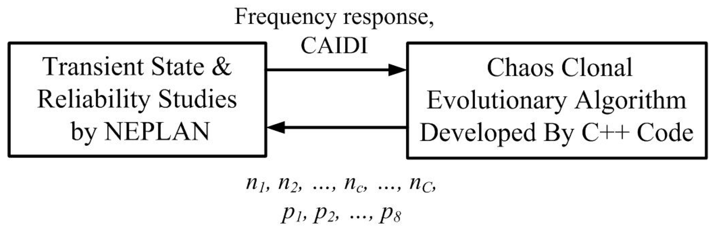
In the above formulation, ${\widehat{a}}_i$ = [a_i1, a_i2, …, a_ij, …, a_iJ] (i.e., ${\widehat{a}}_i$ = [Z, n₁, n₂, …, n_c, …, n_C, p₁, p₂, …, p₈] are decision (independent) variables while CAIDI $f_2\left(\widehat{p}, \widehat{n}\right)$, the lowest swing frequency $f_3\left(\widehat{p}, \widehat{n}\right)$ and the actual total shed load $f_4\left(\widehat{p}, \widehat{n}\right)$ are dependent variables. The other parameters are all known. The chaos clonal evolutionary algorithm determines the values of the decision variables in each iteration. The commercial software NEPLAN 5.5.0, Country [35] is used to evaluate $f_3\left(\widehat{p}, \widehat{n}\right) \mathrm{and} f_4\left(\widehat{p}, \widehat{n}\right).$ The chaos clonal evolutionary algorithm is developed using C++ code. The overall method was implemented using co-simulation, as shown in Figure 2, as follows:

Step 1:

Find $f_{\ell }^{max}$ and $f_{\ell }^{min}, \ell$ = 1, 2, 3, 4.

Step 2:

Specify $f_{\ell }^{*}$, $\ell$ = 1, 2, 3, 4, defined in Section 2.7.

Step 3:

Compute weighting factors for $f_{\ell }$, $\ell$ = 1, 2, 3, 4, according to Equation (21).

Step 4:

Generate feasible antibody ${\widehat{a}}_i$, i = 1, 2, …, NA. (NA = 20 herein)

Step 5:

Estimate antigen affinity (Z) and antibody affinity by Equation (23) for each i, i = 1, 2, …, NA.

Step 6:

Conduct the clone operation by Equation (24).

Step 7:

Execute genetic chaos operation by applying Equations (25)–(27) to reproduce feasible ${\widehat{a}}_i$, i = 1, 2, …, NC.

Step 8:

Let i = 1.

Step 9:

Compute $f_1\left(\widehat{p}, \widehat{n}\right)$ $\mathrm{and} f_2\left(\widehat{p}, \widehat{n}\right)$ directly. $f_3\left(\widehat{p}, \widehat{n}\right)$ $\mathrm{and} f_4\left(\widehat{p}, \widehat{n}\right)$ are calculated using NEPLAN 5.5.0.

Step 10:

If any inequality constraint in Equations (17) and (20) is violated, then calculate its penalty function by (28) and add this penalty function to the corresponding antigen Z.

Step 11:

i = i + 1. If $i>NC,$ then conduct Step 12; otherwise go to Step 9.

Step 12:

Select NA mutated antibodies using the roulette wheel selection that is described in Section 3.6.

Step 13:

If the antibodies are not convergent for the given $f_{\ell }^{*}$, $\ell$ = 1, 2, 3, 4, then go to Step 5.

Step 14:

If the decision-maker is satisfied with the optimal antibody, then output this Pareto optimum; otherwise, go to Step 2.

4. Simulation Results

4.1. Studied System

In this section, a 15-bus standalone power system, which is the first outdoor microgrid test bed in Taiwan, is used in simulations. Figure 3 presents the one-line diagram of this power system. The microgrid test bed has high-concentration PV (HCPV, 60, 31.5, 10 kW) arrays, a wind turbine generator (WTG, 25 kW) and three gas-turbine generator (GTG, 65 kW × 3). The total system load is 180 kW. Many national energy projects have being implemented to explore critical technologies, such as power inverters, blades, PV cells, static switches, and protective devices. Preliminary studies of the operation mode and power quality can be found elsewhere [41,42]. This paper addresses solely determination of BESS while designing the parameters of underfrequency relays. Buses 2, 5, 6, 8–10 and 12–15 are the candidate buses for the installation of batteries, so C = 10. The power of a battery unit is 3 kW, and $n_c^{max}=3$ and $n_c^{min}=0.$ The frequencies in different stages of the underfrequency relays are 58.8 (=98% × 60 Hz), 58.0 (=97% × 60 Hz), …, 54.6 (=91% × 60 Hz). The maximum shed load is 30% of 180 kW, which is 54 kW.

Table 1. Failure rate (occ./year) and annual outage duration (h/year).

Components	Failure Rate (occ./year)	Annual Outage Duration (h/year)
Micro-turbine generator	0.18	12
PV module	0.12	72
Wind-turbine generator	0.22	60
BESS	0.12	1
Transformer	0.0504	168

presents the failure rates (occurrence/year) and annual outage durations (h/year) of different components. The worst scenario is considered in setting the parameters of the underfrequency relays. In this scenario, the load is the peak load (180 kW) and the corresponding kW outputs of the distributed generations are shown in

Table 2. Real power outputs from different distributed generations.

Distributed Generators	Zone 1 (Buses 2–6)	Zone 2 (Buses 8–11)	Zone 3 (Buses 12–17)
Micro-turbine generator	40 kW	65 kW	45 kW
PV module	10 kW	5 kW	5 kW
Wind-turbine generator	-	-	15 kW

. When the gas-turbine generator (65 kW) at bus 11 is lost, the system frequency declines more severely than with the loss of any other micro-turbine generators.

4.2. Comparative Results

The proposed method and the traditional genetic algorithm, which uses classical crossover, mutation and selection operations [40], are utilized to study the worst scenario, which is defined in Section 4.1.

Table 3. Preferred values $f_{\ell }^{*}$ and corresponding weighting factors.

	${\mathit{f}}_{\mathbf{1}}^{*}$ (No. of BESS)	${\mathit{f}}_{\mathbf{2}}^{*}$ (h/occ.)	${\mathit{f}}_{\mathbf{3}}^{*}$ (Hz)	${\mathit{f}}_{\mathbf{4}}^{*}$ (kW)
Preferred values	5.0	45.5	58.8	21.6
Normalized bases	30	70	60	54
Normalized values	0.17	0.65	0.98	0.4
Weighting factors	0.208	0.088	0.005	0.150

presents the preferred values $f_{\ell }^{*}$, $\ell =1, 2, 3, 4,$ and their corresponding weighting factors, calculated using Equation (21). The population size in the genetic algorithm is 20, which is the same as the number of antibodies (NA). The crossover rate and mutation rate in the genetic algorithm are 0.8 and 0.1, respectively. The performance of each method is evaluated by running ten simulations.

Table 4. Mean values of least upper bound Z and $f_{\ell }$.

Method	Z	${\mathit{f}}_{\mathbf{1}}$ (No. of BESS)	${\mathit{f}}_{\mathbf{2}}$ (h/occ.)	${\mathit{f}}_{\mathbf{3}}$ (Hz)	${\mathit{f}}_{\mathbf{4}}$ (kW)
GA	0.016	6.10	42.27	58.56	23.01
Proposed method	0.009	4.60	46.04	58.56	22.89

presents the mean (average value) of BESS, CAIDI, lowest swing frequency and shed load obtained by both methods. Table 4 reveals that the least upper bound Z, $f_1$ and $f_4$ that are obtained using the proposed method are better than those obtained using the genetic algorithm. Both methods approach the same value of $f_3$.

Table 5. Results obtained using genetic algorithm and the proposed method.

Method	Z	n1 at bus 2	n2 at bus 5	n3 − n10
Genetic algorithm	0.013	3	3	0
Proposed method	0.009	3	1	0

and

Table 6. Results obtained using genetic algorithm and the proposed method.

Method	p1 (kW)	p2 (kW)	p3 (kW)	p4 (kW)	p5 − p8 (kW)
Genetic algorithm	26.34	8.88	8.24	6.00	(very small)
Proposed method	22.51	22.17	2.41	2.15	0.00

illustrate the best results (smallest Z) that were obtained using the proposed method and genetic algorithm. As indicated in Table 5, the optimal Z and the total number of batteries (n₁ + n₂) that were obtained using the proposed method are better than those obtained using the genetic algorithm. Since the proposed method yields fewer batteries, it estimates a slightly larger CAIDI (46.04 vs. 42.27 h/occurence). The loads are shed in the first stage actually although the shed loads in all stages are estimated. Figure 4 and Figure 5 plots the frequency responses obtained using both methods when the first-stage loads are shed. The genetic algorithm shed a greater load and yields a smaller swing frequency.

4.3. Impact of Population Size (NA)

The results in Section 4.2 are based on NA = 20. This section investigates the impact of the population size (NA = 10, 20 and 30) on the performance of the method used to find the solution. Again, 10 runs are carried out for each NA.

Table 7. Mean values of least upper bound Z and $f_{\ell }$ for different NA.

NA	Z	${\mathit{f}}_{\mathbf{1}}$ (No. of BESS)	${\mathit{f}}_{\mathbf{2}}$ (h/occ.)	${\mathit{f}}_{\mathbf{3}}$ (Hz)	${\mathit{f}}_{\mathbf{4}}$ (kW)
10	0.009	4.8	45.467	58.56	23.04
20	0.009	4.6	46.040	58.56	22.89
30	0.009	4.3	46.889	58.53	21.33

presents the average values of least upper bound Z and $f_{\ell }$ for different NA. The result obtained using the proposed method is nearly independent of the number of antibodies (NA).

4.4. Impact of Different $f_{\ell }^{*}$

This section examines the effects of the preferred values $f_{\ell }^{*}$ on the solutions. NA is fixed at 20 and ten runs are conducted for each set of preferred $f_{\ell }^{*}.$ Five sets of $f_{\ell }^{*}$ are discussed. The first case serves as a reference in the following discussion.

(i)

$f_2^{*}$ is higher in Case 2 than that in Case 1, increasing f₂ and reducing f₁. Since the mean number of batteries is reduced to 4.6, more load (f₄) is shed and the swing frequency (f₃) is higher.

(ii)

$f_1^{*}$ is increased in Case 3, compared with that in Case 1. This leads to an increase in f₁ and decrease in f₂ substantially. Since more batteries are needed, less load (f₄) is shed and the swing frequency (f₃) is higher.

(iii)

$f_3^{*}$ is increased in Case 4 from that in Case 1. Consequently, more load (f₄) has to be shed and fewer batteries (f₁) are required. Additionally, the fewer batteries make the microgrid less reliable (see f₂).

(iv)

$f_4^{*}$ is higher in Case 5 than that in Case 1. More loads (f₄) are shed and the swing frequency (f₃) is higher. Since more loads (f₄) are expected to be shed, fewer batteries (f₁) may suffice and reliability is reduced (higher f₂).

(v)

$f_1$ is the most sensitive to its variation of preferred value as can be seen in Case 4; $f_3$ is the least sensitive to its variation of preferred value.

Table 8. Mean values of least upper bound Z and $f_{\ell }$ for different $f_{\ell }^{*}$.

Case	Preferred Values	Z	${\mathit{f}}_{\mathbf{1}}$ (No. of BESS)	${\mathit{f}}_{\mathbf{2}}$ (h/yr)	${\mathit{f}}_{\mathbf{3}}$ (Hz)	${\mathit{f}}_{\mathbf{4}}$ (kW)
1	$f_1^{*}$ = 5, $f_2^{*}$ = 35 h/y, $f_3^{*}$ = 58.2 Hz, $f_4^{*}$ = 21.6 kW	0.017	5.7	43.189	58.536	21.927
2	$f_1^{*}$ = 5, $f_2^{*}$ = 45.5 h/y, $f_3^{*}$ = 58.2 Hz, $f_4^{*}$ = 21.6 kW	0.009	4.6	46.035	58.557	23.055
3	$f_1^{*}$ = 10, $f_2^{*}$ = 35 h/y, $f_3^{*}$ = 58.2 Hz, $f_4^{*}$ = 21.6 kW	0.009	9.6	35.315	58.518	20.749
4	$f_1^{*}$ = 5, $f_2^{*}$ = 35 h/y, $f_3^{*}$ = 58.8 Hz, $f_4^{*}$ = 21.6 kW	0.017	5.4	43.917	58.555	23.168
5	$f_1^{*}$ = 5, $f_2^{*}$ = 35 h/y, $f_3^{*}$ = 58.2 Hz, $f_4^{*}$ = 32.4 kW	0.017	5.1	44.645	58.648	28.477

shows the interactive process that is performed by a decision-maker who assigns his/her preferred $f_{\ell }^{*}.$ The interactive process may be terminated when the decision-maker is satisfied with the results. All of the results are Pareto optimums.

5. Conclusions

This paper proposes a novel method for optimizing the capacities of battery energy storage systems. Both steady-state constraints and dynamic constraints are considered in this multi-objective programming problem. Compared with traditional methods, the proposed method can determine the shed load in each stage of the underfrequency relays and CAIDI while considering new energy storage systems. Since the dynamic lowest swing frequency cannot be expressed as a function, traditional gradient-based optimization methods cannot be used and a new optimizer that is based on the chaos clonal evolutionary algorithm is used to conduct a co-simulation between C++ code and NEPLAN software. The simulation results of an islanded microgrid reveal that the optimal least upper bound and the total number of batteries obtained using the proposed method are lower than those obtained using the genetic algorithm. The genetic algorithm yield a greater shed load and a smaller swing frequency. The proposed method is also robust against variations in population size (number of antibodies). The number of batteries for storing energy is the most sensitive to its variation of the preferred value while the lowest swing frequency is the least sensitive.

References

1. Lasseter, R.H.; Eto, J.H.; Schenkman, B.; Stevens, J.; Vollkommer, H.; Klapp, D.; Linton, E.; Hurtado, H.; Roy, J. CERTS Microgrid Laboratory Test Bed. IEEE Trans. Power Deliv. 2011, 26, 325–332. [Google Scholar] [CrossRef]
2. Lasseter, R.H.; Eto, J. Value and Technology Assessment to Enhance the Business Case for the CERTS Microgrid; DE-FC02-06CH11350; US Department of Energy: Washington, DC, USA, 2010.
3. Colson, C.M.; Nehrir, M.H. Comprehensive real-time microgrid power management and control with distributed agents. IEEE Trans. Smart Grid 2013, 4, 617–627. [Google Scholar] [CrossRef]
4. Hong, Y.Y.; Lai, Y.M.; Chang, Y.R.; Lee, Y.D.; Liu, P.W. Optimizing Capacities of Distributed Generation and Energy Storage in a Small Autonomous Power System Considering Uncertainty in Renewables. Energies 2015, 8, 2438–2457. [Google Scholar] [CrossRef]
5. Poullikkas, A. A comparative overview of large-scale battery systems for electricity storage. Renew. Sustain. Energy Rev. 2013, 27, 778–788. [Google Scholar] [CrossRef]
6. Keyhani, A. Design of Smart Power Grid Renewable Energy Systems; Wiley-IEEE Press: Hoboken, NJ, USA, 2011. [Google Scholar]
7. Capstone Turbine Corporation. Capstone MicroTurbine Model C65 User’s Manual; Capstone Turbine Corporation: Los Angeles, CA, USA, 2007. [Google Scholar]
8. Gaonkar, D.N.; Patel, R.N.; Pillai, G.N. Dynamic model of micro-turbine generation system for grid connected/islanding operation. In Proceedings of the IEEE International Conference on Industrial Technology, Bhubaneswar, India, 15–17 December 2006; pp. 305–310. [Google Scholar]
9. Quesada, J.; Sebastián, R.; Castro, M.; Sainz, J.A. Control of inverters in a low-voltage microgrid with distributed battery energy storage. Part II: Secondary control. Electr. Power Syst. Res. 2014, 114, 136–145. [Google Scholar] [CrossRef]
10. Serban, I.; Marinescu, C. Battery energy storage system for frequency support in microgrids and with enhanced control features for uninterruptible supply of local loads. Int. J. Electr. Power Energy Syst. 2014, 54, 432–441. [Google Scholar] [CrossRef]
11. Cho, S.M.; Yun, S.Y. Optimal power assignment of energy storage systems to improve the energy storage efficiency for frequency regulation. Energies 2017, 10, 2092. [Google Scholar] [CrossRef]
12. Daud, M.Z.; Mohamed, A.; Hannan, M.A. An improved control method of battery energy storage system for hourly dispatch of photovoltaic power sources. Energy Convers. Manag. 2013, 73, 256–270. [Google Scholar] [CrossRef]
13. Koohi-Kamali, S.; Rahim, N.A.; Mokhlis, H. Smart power management algorithm in microgrid consisting of photovoltaic, diesel, and battery storage plants considering variations in sunlight, temperature, and load. Energy Convers. Manag. 2014, 84, 562–582. [Google Scholar] [CrossRef]
14. Khalid, M.; Savkin, A.V. Minimization and control of battery energy storage for wind power smoothing: Aggregated, distributed and semi-distributed storage. Renew. Energy 2014, 64, 105–112. [Google Scholar] [CrossRef]
15. Mehdi, D.; Jamel, B.; Xavier, R. Hybrid solar-wind system with battery storage operating in grid–connected and standalone mode: Control and energy management—Experimental investigation. Energy 2010, 35, 2587–2595. [Google Scholar]
16. Mohsen, G.; Hamid, F. Battery capacity determination with respect to optimized energy dispatch schedule in grid-connected photovoltaic (PV) systems. Energy 2014, 65, 665–674. [Google Scholar]
17. Maleki, A.; Askarzadeh, A. Optimal sizing of a PV/wind/diesel system with battery storage for electrification to an off-grid remote region: A case study of Rafsanjan, Iran. Sustain. Energy Technol. Assess. 2014, 7, 147–153. [Google Scholar] [CrossRef]
18. Ma, T.; Yang, H.X.; Lu, L. A feasibility study of a stand-alone hybrid solar–wind–battery system for a remote island. Appl. Energy 2014, 121, 149–158. [Google Scholar] [CrossRef]
19. Bernal-Agustin, J.L.; Dufo-Lopez, R. Simulation and optimization of stand-alone hybrid renewable energy systems. Renew. Sustain. Energy Rev. 2009, 13, 2111–2118. [Google Scholar] [CrossRef]
20. Ekren, O.; Ekren, B.Y. Size optimization of a PV/wind hybrid energy conversion system with battery storage using simulated annealing. Appl. Energy 2010, 87, 592–598. [Google Scholar] [CrossRef]
21. Ekren, B.Y.; Ekren, O. Simulation based size optimization of a PV/wind hybrid energy conversion system with battery storage under various load and auxiliary energy conditions. Appl. Energy 2009, 86, 1387–1394. [Google Scholar] [CrossRef]
22. Mohammadi, S.; Mohammadi, A. Stochastic scenario-based model and investigating size of battery energy storage and thermal energy storage for micro-grid. Electr. Power Energy Syst. 2014, 61, 531–546. [Google Scholar] [CrossRef]
23. Quevedo, P.M.; Contreras, J. Optimal placement of energy storage and wind power under uncertainty. Energies 2016, 9, 528. [Google Scholar] [CrossRef]
24. Han, X.; Liao, S.; Ai, X.; Yao, W.; Wen, J. Determining the minimal power capacity of energy storage to accommodate renewable generation. Energies 2017, 10, 468. [Google Scholar] [CrossRef]
25. Rei, A.M.; Leite da Silva, A.M.; Jardim, J.L.; Mello, J.C.O. Static and dynamic aspects in bulk power system reliability evaluations. IEEE Trans. Power Syst. 2000, 15, 189–195. [Google Scholar] [CrossRef]
26. Huishi, L.; Jian, S.; Sige, L. Reliability evaluation of distribution system containing microgrid. In Proceedings of the China International Conference on Electricity Distribution (CICED), Nanjing, China, 13–16 September 2010. [Google Scholar]
27. Rostamirad, S.; Wang, K.; Marti, J.R. Power management in disasters: Application of load shedding and wind turbine controller. In Proceedings of the 24th Canadian Conference on Electrical and Computer Engineering, Niagara Falls, ON, Canada, 8–11 May 2011; pp. 1511–1514. [Google Scholar]
28. Sigrist, L.; Egido, I.; Rouco, L. A method for the design of UFLS schemes of small isolated power systems. IEEE Trans. Power Syst. 2012, 27, 951–958. [Google Scholar] [CrossRef]
29. Du, H.F.; Gong, M.G.; Liu, R.C.; Jiao, L.C. Adaptive chaos clonal evolutionary programming algorithm. Sci. China Ser. F Inf. Sci. 2005, 48, 579–595. [Google Scholar] [CrossRef]
30. Institute of Electrical and Electronics Engineers (IEEE). IEEE Guide for Electric Power Distribution Reliability Indices; IEEE Standard 1366; IEEE: Piscataway, NJ, USA, 2003. [Google Scholar]
31. Endrenyi, J. Reliability Modeling in Electric Power Systems; John Wiley & Sons: Hoboken, NJ, USA, 1979. [Google Scholar]
32. Manson, S.; Zweigle, G.; Yedidi, V. Case study: An adaptive underfrequency load-shedding system. IEEE Trans. Ind. Appl. 2014, 50, 1659–1667. [Google Scholar] [CrossRef]
33. Joo, S.K.; Liu, C.C.; Jones, L.E.; Choe, J.W. Coherency and aggregation techniques incorporating rotor and voltage dynamics. IEEE Trans. Power Syst. 2004, 19, 1068–1075. [Google Scholar] [CrossRef]
34. Wang, L.; Truong, D.N. Dynamic stability improvement of four parallel-operated PMSG-based offshore wind turbine generators fed to a power system using a STATCOM. IEEE Trans. Power Deliv. 2013, 28, 111–119. [Google Scholar] [CrossRef]
35. NEPLAN V5.5.0 User Manual; NEPLAN AG: Zürich, Switzerland, 2012.
36. Task Force on Turbine-Governor, Power System Dynamic Performance Committee. Dynamic Models for Turbine-Governors in Power System Studies; IEEE PES: Piscataway, NJ, USA, 2014. [Google Scholar]
37. Ammar, E.I. Interactive stability of multiobjective NLP problems with fuzzy parameters in the objective functions and constraints. Fuzzy Sets Syst. 2000, 19, 83–90. [Google Scholar] [CrossRef]
38. Chankong, V.; Haimes, Y. Multiobjective Decision Making Theory and Methodology; North-Holland Series in System Science and Engineering; Courier Dover Publications: Mineola, NY, USA, 1983. [Google Scholar]
39. Edward, N.L. Designing chaotic models. J. Atmos. Sci. 2005, 62, 1574–1587. [Google Scholar]
40. Gen, M.; Cheng, R. Genetic Algorithms and Engineering Design; John Wiley & Sons, Inc.: New York, NY, USA, 1997. [Google Scholar]
41. Hong, Y.Y.; Su, D.S.; Hsiao, M.C.; Chang, Y.R.; Lee, Y.D.; Cheng, C.M. Preliminary studies on first outdoor microgrid test bed in Taiwan. In Proceedings of the 2011 IEEE Trondheim PowerTech, Trondheim, Norway, 19–23 June 2011. [Google Scholar]
42. Hong, Y.Y.; Lai, Y.Z.; Hsiao, M.C.; Chang, Y.R.; Lee, Y.D.; Huang, H.C. Studies on operation modes for the first outdoor microgrid test bed in Taiwan. In Proceedings of the IEEE International Conference on Power System Technology (POWERCON), Auckland, New Zealand, 30 October–2 November 2012. [Google Scholar]
Figure 1. The gas-turbine model [36].
Energies 11 00585 g001
Figure 2. Co-simulation conducted in the proposed method.
Energies 11 00585 g002
Figure 3. One-line diagram of the studied microgrid.
Energies 11 00585 g003
Figure 4. System frequency response obtained using genetic algorithm.
Energies 11 00585 g004
Figure 5. System frequency response obtained using proposed method.
Energies 11 00585 g005