Methods of Decline Curve Analysis for Shale Gas Reservoirs


Abstract
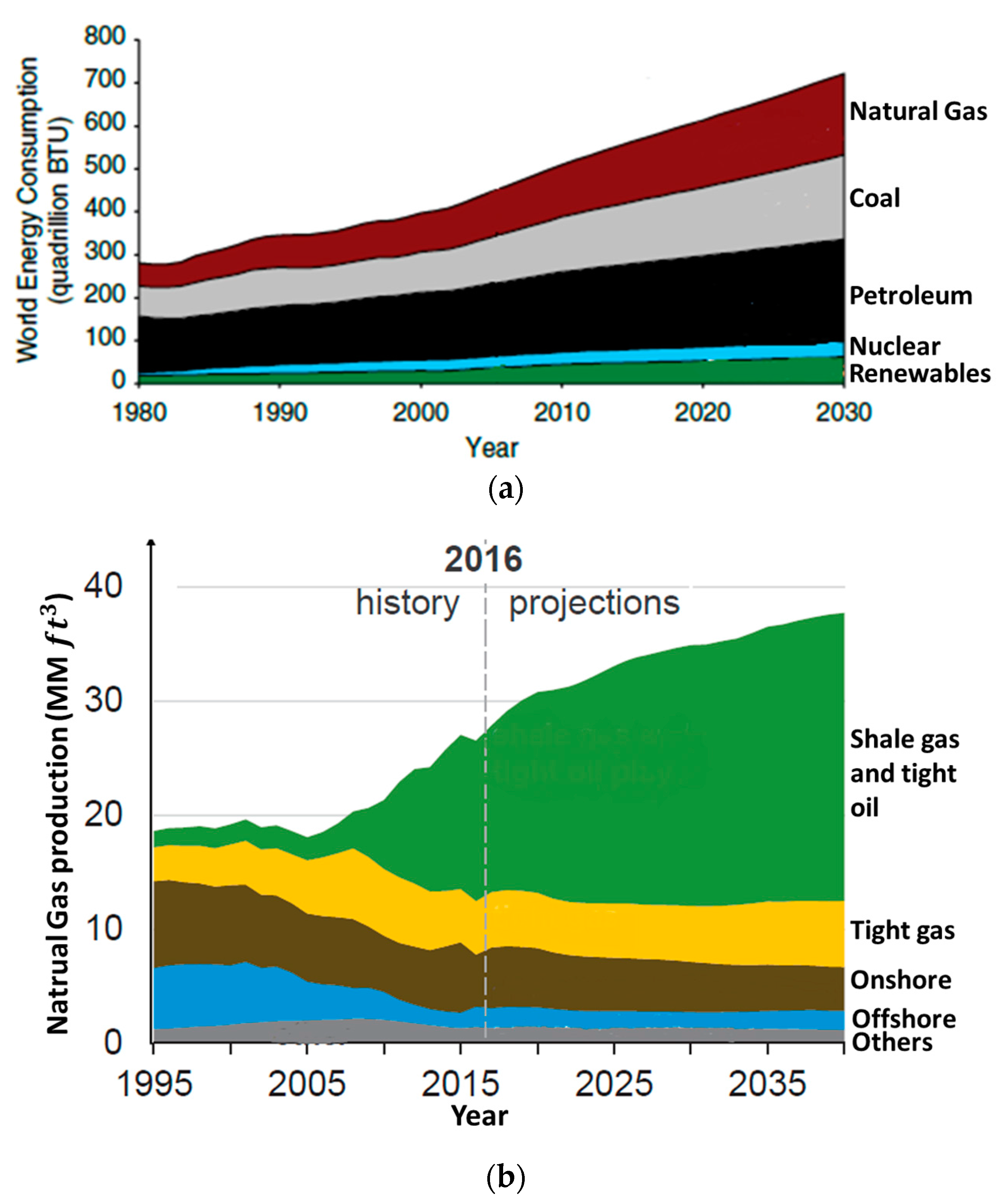
:1. Introduction
2. DCA Models and Applications
2.1. Origins of DCA
2.2. Arps Decline Model
2.3. Modified Hyperbolic Decline Model
2.4. Power Law Exponential Decline Model
2.5. Stretched Exponential Decline Model
2.6. Duong Model
2.7. Logistic Growth Model
2.8. Extended Exponential DCA Model
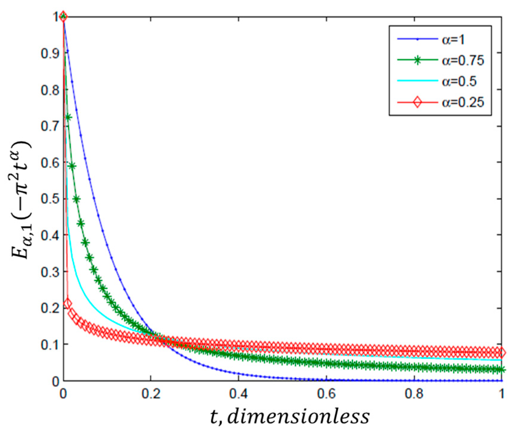
2.9. Fractional Decline Curve Model
2.10. Probabilistic Decline Curve Model
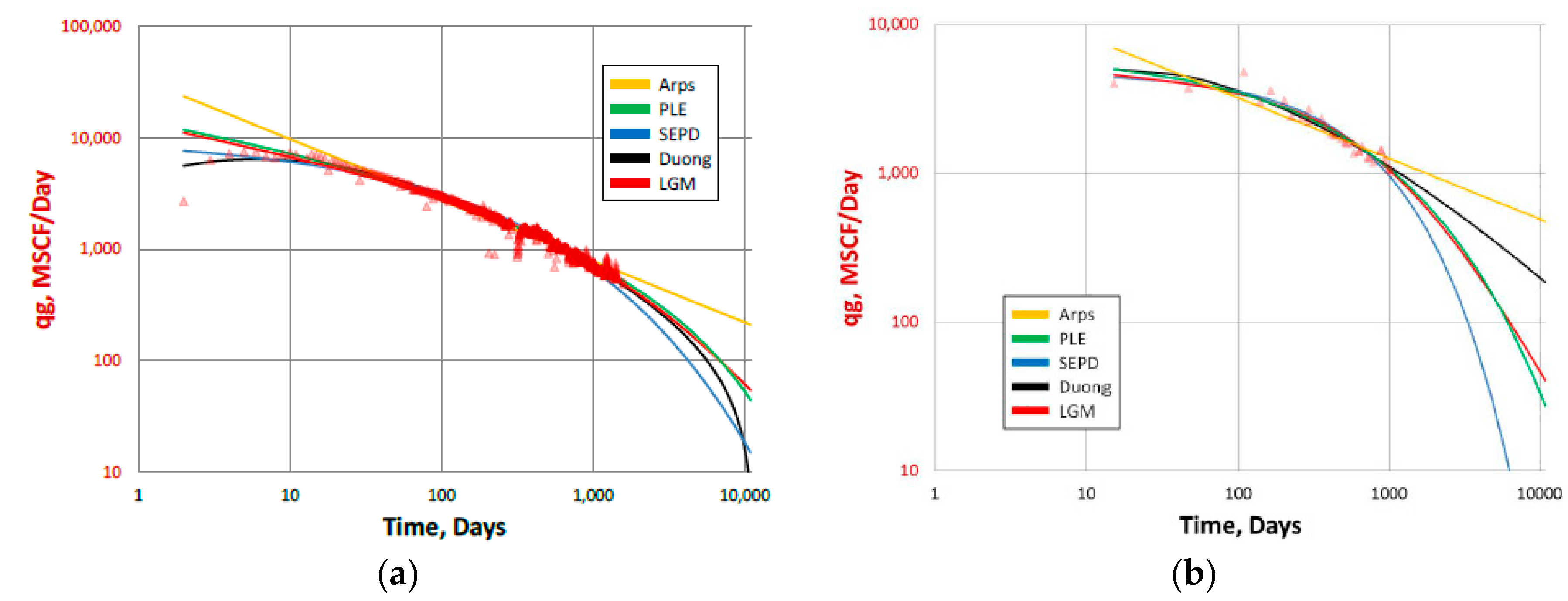
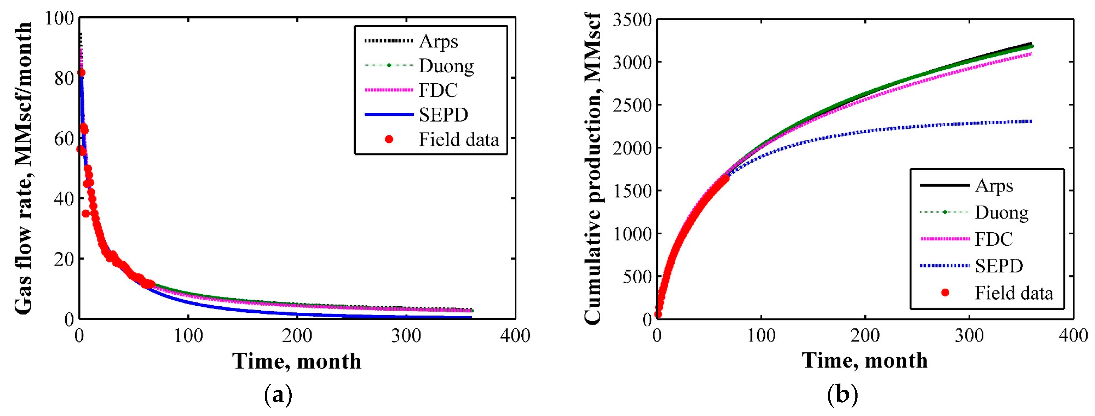
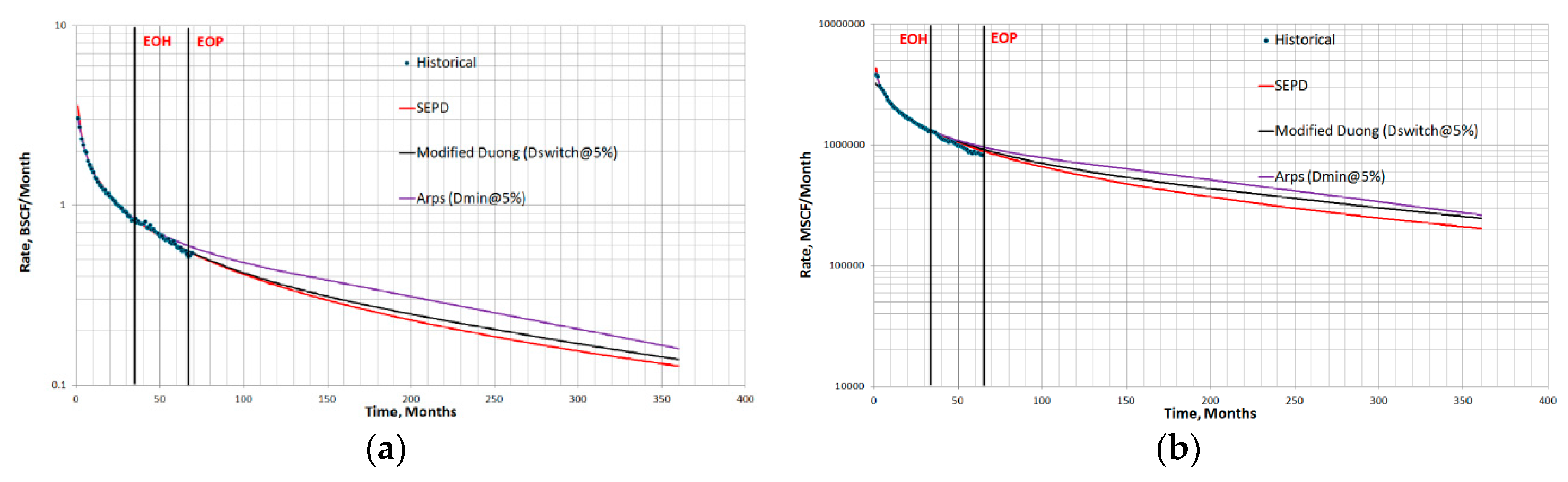
2.11. Comparisons of DCA Models with Field Data
3. Discussion
4. Conclusions
Acknowledgments
Author Contributions
Conflicts of Interest
References
- EIA. International Energy Outlook; EIA: Washington, DC, USA, 2017.
- EIA. Annual Energy Outlook; EIA: Washington, DC, USA, 2017.
- An, C.; Yan, B.; Alfi, M.; Mi, L.; Killough, J.E.; Heidari, Z. Estimating spatial distribution of natural fractures by changing NMR T2 relaxation with magnetic nanoparticles. J. Petrol. Sci. Eng. 2017, 157, 273–287. [Google Scholar] [CrossRef]
- Lohr, S.C.; Baruch, E.T.; Hall, P.A.; Kennedy, M.J. Is organic pore development in gas shales influenced by the primary porosity and structure of thermally immature organic matter? Organ. Geochem. 2015, 87, 119–132. [Google Scholar] [CrossRef]
- Wu, K.L.; Li, X.F.; Wang, C.C.; Yu, W.; Chen, Z.X. Model for surface diffusion of adsorbed gas in nanopores of shale gas reservoirs. Ind. Eng. Chem. Res. 2015, 54, 3225–3236. [Google Scholar] [CrossRef]
- Wang, K.; Liu, H.; Luo, J.; Wu, K.L.; Chen, Z.X. A comprehensive model coupling embedded discrete fractures, multiple interacting continua, and geomechanics in shale gas reservoirs with multiscale fractures. Energy Fuel 2017, 31, 7758–7776. [Google Scholar] [CrossRef]
- Wu, K.L.; Chen, Z.X.; Li, J.; Li, X.F.; Xu, J.Z.; Dong, X.H. Wettability effect on nanoconfined water flow. Proc. Natl. Acad. Sci. USA 2017, 114, 3358–3363. [Google Scholar] [CrossRef] [PubMed]
- Zuo, L.H.; Chen, W. Double layer potential method for the spontaneous well-logging. Chin. J. Eng. Math. 2008, 25, 1013–1022. [Google Scholar]
- Li, H.; Wang, H. Investigation of eccentricity effects and depth of investigation of azimuthal resistivity lwd tools using 3D finite difference method. J. Petrol. Sci. Eng. 2016, 143, 211–225. [Google Scholar] [CrossRef]
- Wang, H.; Fehler, M. The wavefield of acoustic logging in a cased hole with a single casing—Part II: A dipole tool. Geophys. J. Int. 2018, 212, 1412–1428. [Google Scholar] [CrossRef]
- Wang, H.; Fehler, M. The wavefield of acoustic logging in a cased-hole with a single casing—Part I: A monopole tool. Geophys. J. Int. 2018, 212, 612–626. [Google Scholar] [CrossRef]
- Kanfar, M.S.; Wattenbarger, R.A. Comparison of Empirical Decline Curve Methods for Shale Wells. In Proceedings of the SPE Canadian Unconventional Resources Conferences, Calgary, AB, Canada, 30 October–1 November 2012. [Google Scholar]
- Joshi, L.; Lee, J. Comparison of various deterministic forecasting techniques in shale gas reservoirs. In Proceedings of the SPE Hydraulic Fracturing Technology Conference, The Woodlands, TX, USA, 4–6 February 2013. [Google Scholar] [CrossRef]
- Lee, W.J. Critique of Simple Decline Models; SPE Webinar: Richardson, TX, USA, 2015. [Google Scholar]
- Hu, Y.; Weijermar, R.; Zuo, L.H.; Yu, W. Benchmarking eur estimates for hydraulically fractured wells with and without fracture hits using various dca methods. J. Petrol. Sci. Eng. 2017, in press. [Google Scholar] [CrossRef]
- Arnold, R.; Anderson, R. Preliminary Report on Coalinga Oil District, Fresno and Kings Counties, U.S. Geological Survey Bulletin; US Government Printing Office: Washington, DC, USA, 1908.
- Arnold, R. Two decades of petroleum geology, 1903–1922. AAPG Bull. 1923, 7, 603–624. [Google Scholar]
- Johnson, R.H.; Bollens, A.L. The loss ratio method of extrapolating oil well decline curves. Trans. Am. Inst. Min. Metall. Eng. 1927, 77, 771–778. [Google Scholar] [CrossRef]
- Cutler, W.W.; Johnson, H.R. Estimating Recoverable Oil of Curtailed Wells; Oil Weekly: Houston, TX, USA, 1940. [Google Scholar]
- Arps, J.J. Analysis of decline curves. Trans. Am. Inst. Min. Metall. Eng. 1945, 160, 228–247. [Google Scholar] [CrossRef]
- Akbarnejad-Nesheli, B.; Valko, P.; Lee, J.W. Relating fracture network characteristics to shale gas reserve estimation. In Proceedings of the SPE Americas Unconventional Resources Conference, Pittsburgh, PA, USA, 5–7 June 2012. [Google Scholar] [CrossRef]
- Mattar, L.; Gault, B.; Morad, K.; Clarkson, C.R.; Freeman, C.M.; IIK, D.; Blasingame, T.A. Production analysis and forecasting of shale gas reservoirs: Case history-based approach. In Proceedings of the SPE Shale Gas Production Conference, Fort Worth, TX, USA, 16–18 November 2008. [Google Scholar] [CrossRef]
- Shahamat, M.S.; Mattar, L.; Aguilera, R. Analysis of decline curves on the basis of beta-derivative. SPE Reserv. Eval. Eng. 2015, 18, 214–227. [Google Scholar] [CrossRef]
- Clarkson, C.R.; Qanbari, F.; Williams-Kovacs, J.D. Innovative use of rate-transient analysis methods to obtain hydraulic-fracture properties for low-permeability reservoirs exhibiting multiphase flow. Lead. Edge Spec. Sect. Hydrofract. Mod. Novel Methods 2014, 30, 1108–1122. [Google Scholar] [CrossRef]
- Lee, W.J.; Sidle, R. Gas-reserves estimation in resource plays. SPE Econ. Manag. 2010, 2, 86–91. [Google Scholar] [CrossRef]
- Robertson, S. Generalized Hyperbolic Equation; USMS SPE-18731; Society of Petroleum Engineers: Richardson, TX, USA, 1988. [Google Scholar]
- Seshadri, J.N.; Mattar, L. Comparison of power law and modified hyperbolic decline methods. In Proceedings of the Canadian Unconventional Resources and International Petroleum Conference, Calgary, AB, Canada, 19–21 October 2010. [Google Scholar] [CrossRef]
- Meyet Me Ndong, M.P.; Dutta, R.; Burns, C. Comparison of decline curve analysis methods with analytical models in unconventional plays. In Proceedings of the SPE Annual Technical Conference and Exhibition, New Orleans, LA, USA, 30 September–2 October 2013. [Google Scholar] [CrossRef]
- Paryani, M.; Ahmadi, M.; Awoleke, O.; Hanks, C. Using improved decline curve models for production forecasts in unconventional reservoirs. In Proceedings of the SPE Eastern Regional Meeting, Canton, OH, USA, 13–15 September 2016. [Google Scholar] [CrossRef]
- Ilk, D.; Rushing, J.A.; Perego, A.D.; Blasingame, T.A. Exponential vs. Hyperbolic decline in tight gas sands: Understanding the origin and implications for reserve estimates using arps’ decline curves. In Proceedings of the SPE Annual Technical Conference and Exhibition, Denver, CO, USA, 21–24 September 2008. [Google Scholar] [CrossRef]
- Mattar, L.; Moghadam, S. Modified power law exponential decline for tight gas. In Proceedings of the Canadian International Petroleum Conference, Calgary, AB, Canada, 16–18 June 2009. [Google Scholar]
- McNeil, R.; Jeje, O.; Renaud, A. Application of the power law loss-ratio method of decline analysis. In Proceedings of the Canadian International Petroleum Conference, Calgary, AB, Canada, 16–18 June 2009. [Google Scholar] [CrossRef]
- Valkó, P.P. Assigning value to stimulation in the barnett shale: A simultaneous analysis of 7000 plus production histories and well completion records. In Proceedings of the SPE Hydraulic Fracturing Technology Conference, The Woodlands, TX, USA, 19–21 January 2009. [Google Scholar]
- Valkó, P.P.; Lee, J.W. A better way to forecast production from unconventional gas wells. In Proceedings of the SPE Annual Technical Conference and Exhibition, Florence, Italy, 19–22 September 2010. [Google Scholar] [CrossRef]
- Zuo, L.H.; Yu, W.; Wu, K. A fractional decline curve analysis model for shale gas reservoirs. Int. J. Coal Geol. 2016, 163, 140–148. [Google Scholar] [CrossRef]
- Duong, A.N. Rate-decline analysis for fracture-dominated shale reservoirs. SPE Reserv. Eval. Eng. 2011, 14, 377–387. [Google Scholar] [CrossRef]
- Wang, K.; Li, H.; Wang, J.; Jiang, B.; Bu, C.; Zhang, Q.; Luo, W. Predicting production and estimated ultimate recoveries for shale gas wells: A new methodology approach. Appl. Energy 2017. [Google Scholar] [CrossRef]
- Spencer, R.P.; Coulombe, M.J. Quantitation of hepatic growth and regeneration. Growth 1966, 30, 277. [Google Scholar] [PubMed]
- Clark, A.J.; Lake, L.W.; Patzek, T.W. Production forecasting with logistic growth models. In Proceedings of the SPE Annual Technical Conference and Exhibition, Denver, CO, USA, 30 October–2 November 2011. [Google Scholar] [CrossRef]
- Zhang, H.; Rietz, D.; Cagle, A.; Cocco, M.; Lee, J. Extended exponential decline curve analysis. J. Nat. Gas Sci. Eng. 2016, 36, 402–413. [Google Scholar] [CrossRef]
- Fetkovich, M.J. Decline curve analysis using type curves. J. Pet. Technol. 1980, 32, 1065–1077. [Google Scholar] [CrossRef]
- Chaves, A.S. A fractional diffusion equation to describe levy fights. Phys. Lett. A 1998, 239, 13–16. [Google Scholar] [CrossRef]
- Adams, E.E.; Gelhar, L.W. Field-study of dispersion in a heterogeneous aquifer: 2. Spatial moments analysis. Water Resour. Res. 1992, 28, 3293–3307. [Google Scholar] [CrossRef]
- Sakamoto, K.; Yamamoto, M. Initial value/boundary value problems for fractional diffusion-wave equations and applications to some inverse problems. J. Math. Anal. Appl. 2011, 382, 426–447. [Google Scholar] [CrossRef]
- Nakagawa, J.; Sakamoto, K.; Yamamoto, M. Overview to mathematical analysis for fractional diffusion equations-new mathematical aspects motivated by industrial collaboration. J. Math. Ind. 2010, 2A, 99–108. [Google Scholar]
- Zhou, L.Z.; Selim, H.M. Application of the fractional advection-dispersion equation in porous media. Soil Sci. Soc. Am. J. 2003, 67, 1079–1084. [Google Scholar] [CrossRef]
- Metzler, R.; Klafter, J. The random walk’s guide to anomalous diffusion: A fractional dynamics approach. Phys. Rep. Rev. Sect. Phys. Lett. 2000, 339, 1–77. [Google Scholar] [CrossRef]
- Nigmatullin, R.R. The realization of the generalized transfer equation in a medium with fractal geometry. Phys. Status Solidi B Basic Res. 1986, 133, 425–430. [Google Scholar] [CrossRef]
- Luchko, Y. Maximum principle for the generalized time-fractional diffusion equation. J. Math. Anal. Appl. 2009, 351, 218–223. [Google Scholar] [CrossRef]
- Luchko, Y. Some uniqueness and existence results for the initial-boundary-value problems for the generalized time-fractional diffusion equation. Comput. Math. Appl. 2010, 59, 1766–1772. [Google Scholar] [CrossRef]
- Luchko, Y.; Zuo, L. Θ-function method for a time-fractional reaction-diffusion equation. J. Algerian Math. Soc. 2014, 1, 1–15. [Google Scholar]
- Chen, C.; Raghavan, R. Transient flow in a linear reservoir for space-time fractional diffusion. J. Petrol. Sci. Eng. 2015, 128, 194–202. [Google Scholar] [CrossRef]
- Holy, R.W.; Ozkan, E. Numerical modeling of multiphase flow toward fractured horizontal wells in heterogeneous nanoporous formations. In Proceedings of the SPE Annual Technical Conference and Exhibition, Dubai, UAE, 26–28 September 2016. [Google Scholar]
- Berkowitz, B.; Cortis, A.; Dentz, M.; Scher, H. Modeling non-fickian transport in geological formations as a continuous time random walk. Rev. Geophys. 2006, 44. [Google Scholar] [CrossRef]
- Podlubny, I. Fractional Differential Equations; Academic Press: San Diego, CA, USA, 1999. [Google Scholar]
- Mittag-Leffler, G.M. Sur la nouvelle function eα(x). C. R. Acad. Sci. Paris 1903, 137, 554–558. [Google Scholar]
- Yang, Q.S.; Torres-Verdin, C. Joint interpretation and uncertainty analysis of petrophysical properties in unconventional shale reservoirs. Interpret. J. Subsurf. Charact. 2015, 3, Sa33–Sa49. [Google Scholar] [CrossRef]
- Gelman, A.; Carlin, J.; Stern, H.S.; Dunson, D.B.; Vehtari, A.; Rubin, D.B. Bayesian Data Analysis, 3rd ed.; CRC Press: London, UK; Boca Raton, FL, USA; New York, NY, USA, 2004. [Google Scholar]
- Gong, X.L.; Gonzalez, R.; McVay, D.A.; Hart, J.D. Bayesian probabilistic decline-curve analysis reliably quantifies uncertainty in shale-well-production forecasts. SPE J. 2014, 19, 1047–1057. [Google Scholar] [CrossRef]
- Fulford, D.S.; Bowie, B.; Berry, M.E.; Bowen, B.; Turk, D.W. Machine learning as a reliable technology for evaluating time-rate performance of unconventional wells. In Proceedings of the SPE Annual Technical Conference and Exhibition, Houston, TX, USA, 28–30 September 2015. [Google Scholar]
- Efendiev, Y.; Jin, B.T.; Presho, M.; Tan, X.S. Multilevel markov chain monte carlo method for high-contrast single-phase flow problems. Commun. Comput. Phys. 2015, 17, 259–286. [Google Scholar] [CrossRef]
- Tan, X. Multilevel Uncertainty Quantification Techniques Using Multiscale Methods. Ph.D. Thesis, Texas A&M University, College Station, TX, USA, 2015. [Google Scholar]
- Metropolis, N.; Rosenbluth, M.; Rosenbluth, A.; Teller, A.; Teller, E. Equation of state calculations by fast computer machines. J. Chem. Phys. 1953, 21, 1087–1092. [Google Scholar] [CrossRef]
- Hastings, W.K. Monte-carlo sampling methods using markov chains and their applications. Biometrika 1970, 57, 97–109. [Google Scholar] [CrossRef]
- Cheng, Y.; Wang, Y.; McVay, D.A.; Lee, W.J. Practical application of a probabilistic approach to estimate reserves using production decline data. SPE Econ. Manag. 2010, 2, 19–31. [Google Scholar] [CrossRef]
- Jochen, V.A.; Spivey, J.P. Probabilistic reserves estimation using decline curve analysis with the bootstrap method. In Proceedings of the SPE Annual Technical Conference and Exhibition, Denver, CO, USA, 6–9 October 1996. [Google Scholar]
- Fulford, D.S.; Blasingame, T.A. Evaluation of time-rate performance of shale wells using the transient hyperbolic time-rate relation. In Proceedings of the SPE Unconventional Resources Conference, Calgary, AB, Canada, 5–7 November 2013. [Google Scholar]
- Yu, S. A new methodology to predict condensate production in tight/shale retrograde gas reservoirs. In Proceedings of the SPE Unconventional Resources Conferences, The Woodlands, TX, USA, 1–3 April 2014. [Google Scholar]
- Mondal, A.; Efendiev, Y.; Mallick, B.; Datta-Gupta, A. Bayesian uncertainty quantification for flows in heterogeneous porous media using reversible jump markov chain monte carlo methods. Adv. Water Resour. 2010, 33, 241–256. [Google Scholar] [CrossRef]
- Tierney, L. Markov-chains for exploring posterior distributions. Ann. Stat. 1994, 22, 1701–1728. [Google Scholar] [CrossRef]
- Haario, H.; Saksman, E.; Tamminen, J. An adaptive metropolis algorithm. Bernoulli 2001, 7, 223–242. [Google Scholar] [CrossRef]
- Haario, H.; Laine, M.; Mira, A.; Saksman, E. Dram: Efficient adaptive mcmc. Stat. Comput. 2006, 16, 339–354. [Google Scholar] [CrossRef]
- Goodwin, N. Bridging the gap between deterministic and probabilistic uncertainty quantification using advanced proxy based methods. In Proceedings of the SPE Reservoir Simulation Symposium, Houston, TX, USA, 23–25 February 2015. [Google Scholar]
- Yu, W.; Tan, X.S.; Zuo, L.H.; Liang, J.T.; Liang, H.C.; Wang, S.J. A new probabilistic approach for uncertainty quantification in well performance of shale gas reservoirs. SPE J. 2016, 21, 2038–2048. [Google Scholar] [CrossRef]
- De Holanda, R.W.; Gildin, E.; Valkó, P.P. Combining physics, statistics and heuristics in the decline curve analysis of large datasets in unconventional reservoirs. In Proceedings of the SPE Latin America and Caribbean Petroleum Engineering Conferences, Buenos Aires, Argentina, 18–19 May 2017. [Google Scholar]


| Index | Methods | Year | Decline Curve Expressions | References |
|---|---|---|---|---|
| 1 | Arps Model | 1945 | [20] | |
| 2 | Modified Hyperbolic Decline Model | 1988 | [26] | |
| 3 | Power Law Exponential Decline Model | 2008 | [12,27,28,29,30,32] | |
| 4 | Stretched Exponential Decline Model | 2009 | [33] | |
| 5 | Duong Model | 2011 | [6,12,28,29,35,36] | |
| 6 | Logistic Growth Analysis Model | 2011 | [28,29,39] | |
| 7 | Extended Exponential Decline Curve | 2016 | [40] | |
| 8 | Fractional Decline Model | 2016 | [6,35] |
© 2018 by the authors. Licensee MDPI, Basel, Switzerland. This article is an open access article distributed under the terms and conditions of the Creative Commons Attribution (CC BY) license (http://creativecommons.org/licenses/by/4.0/).
Share and Cite
Tan, L.; Zuo, L.; Wang, B. Methods of Decline Curve Analysis for Shale Gas Reservoirs. Energies 2018, 11, 552. https://doi.org/10.3390/en11030552
Tan L, Zuo L, Wang B. Methods of Decline Curve Analysis for Shale Gas Reservoirs. Energies. 2018; 11(3):552. https://doi.org/10.3390/en11030552
Chicago/Turabian StyleTan, Lei, Lihua Zuo, and Binbin Wang. 2018. "Methods of Decline Curve Analysis for Shale Gas Reservoirs" Energies 11, no. 3: 552. https://doi.org/10.3390/en11030552
APA StyleTan, L., Zuo, L., & Wang, B. (2018). Methods of Decline Curve Analysis for Shale Gas Reservoirs. Energies, 11(3), 552. https://doi.org/10.3390/en11030552