A New Method for Computing the Delay Margin for the Stability of Load Frequency Control Systems


Abstract
1. Introduction
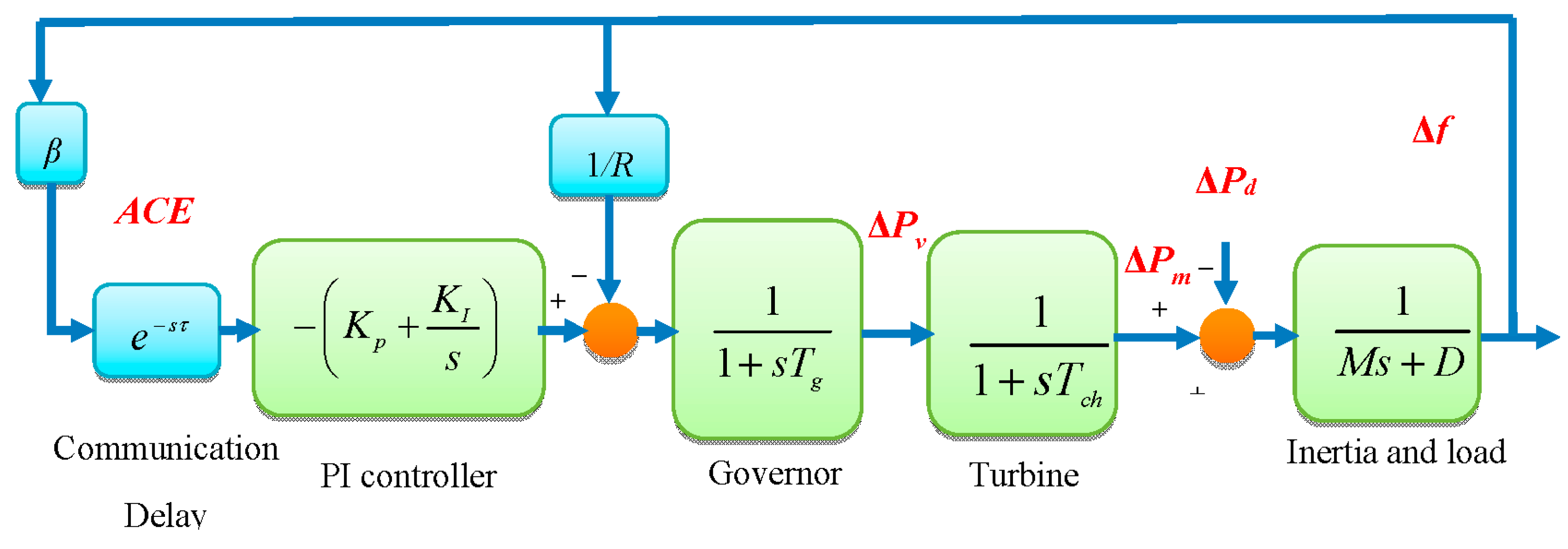
2. Dynamic Model of One-Area LFC System with Time Delay
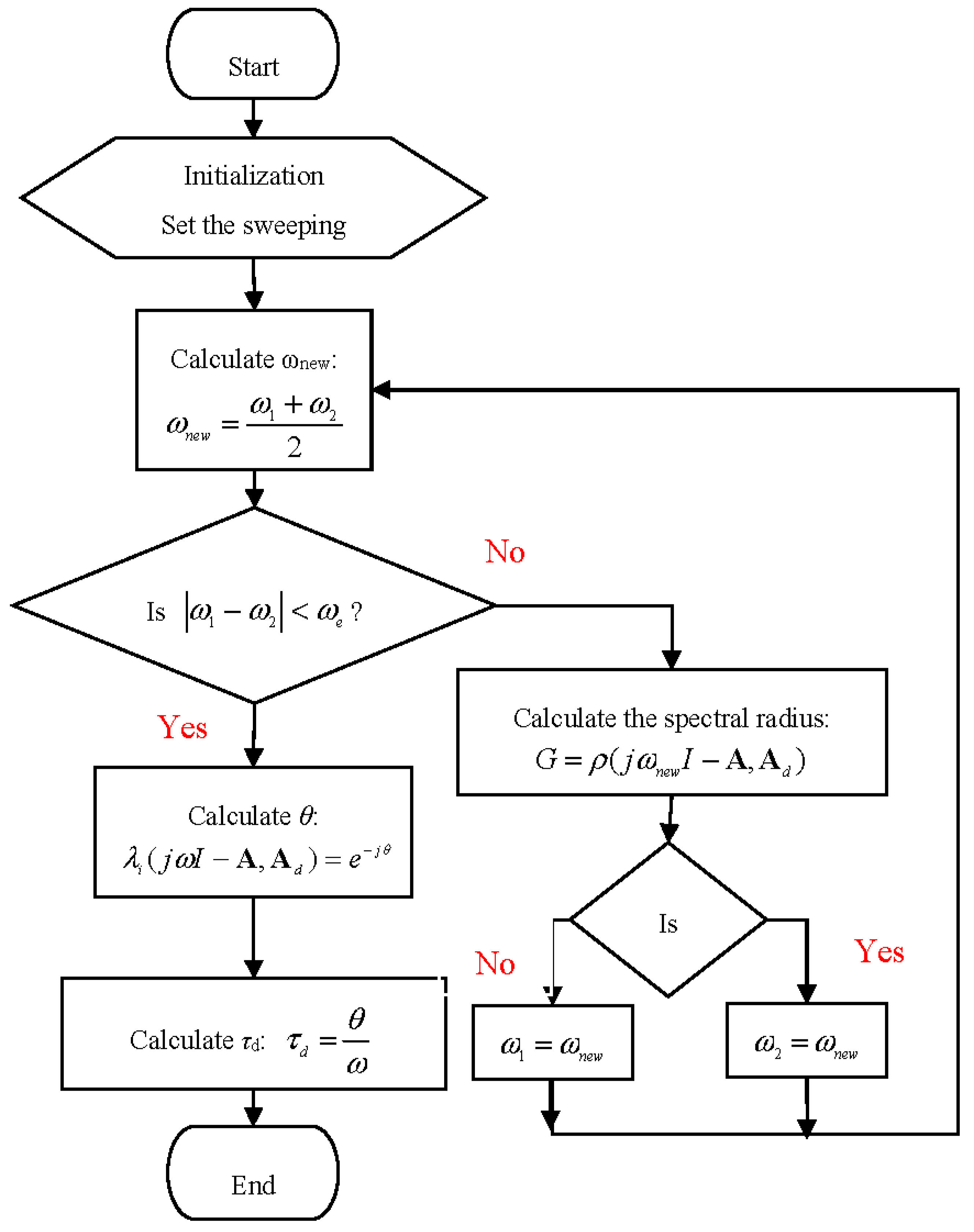
3. Delay Margin Computation Using the Sweeping Test
- (i)
- A is stable,
- (ii)
- A + Ad is stable, and
- (iii)
4. Case Study: One-Area LFC System
5. Conclusions
Author Contributions
Funding
Conflicts of Interest
References
- Saadat, H. Power System Analysis; McGraw-Hill Companies: New York, NY, USA, 1999. [Google Scholar]
- Bhowmik, S.; Tomsovic, K.; Bose, A. Communication Models for Third Party Load Frequency Control. IEEE Trans. Power Syst. 2004, 19, 543–548. [Google Scholar] [CrossRef]
- Khalil, A.; Wang, J.; Mohammed, O. Robust stabilization of load frequency control system under networked environment. Int. J. Autom. Comput. 2017, 14, 93–105. [Google Scholar] [CrossRef]
- Mak, K.H.; Holland, B.L. Migrating electrical power network SCADA systems to TCP/IP and Ethernet networking. Power Eng. J. 2002, 16, 305–311. [Google Scholar]
- Naduvathuparambil, B.; Valenti, M.C.; Feliachi, A. Communication delays in wide area measurement systems. In Proceedings of the Thirty-Fourth Southeastern Symposium on System Theory, Huntsville, Alabama, 18–19 March 2002; pp. 118–122. [Google Scholar]
- Bevrani, H.; Hiyama, T. A control strategy for LFC design with communication delays. In Proceedings of the 2005 International Power Engineering Conference, Singapore, 29 November–2 December 2005; pp. 1087–1092. [Google Scholar]
- Xiaofeng, Y.; Tomsovic, K. Application of linear matrix inequalities for load frequency control with communication delays. IEEE Trans. Power Syst. 2004, 19, 1508–1515. [Google Scholar]
- Zhang, C.K.; Jiang, L.; Wu, Q.H.; He, Y.; Wu, M. Delay-Dependent Robust Load Frequency Control for Time Delay Power Systems. IEEE Trans. Power Syst. 2013, 28, 2192–2201. [Google Scholar] [CrossRef]
- Peng, C.; Zhang, J. Delay-Distribution-Dependent Load Frequency Control of Power Systems with Probabilistic Interval Delays. IEEE Trans. Power Syst. 2016, 31, 3309–3317. [Google Scholar] [CrossRef]
- Zhang, C.K.; Jiang, L.; Wu, Q.H.; He, Y.; Wu, M. Further Results on Delay-Dependent Stability of Multi-Area Load Frequency Control. IEEE Trans. Power Syst. 2013, 28, 4465–4474. [Google Scholar] [CrossRef]
- Dey, R.; Ghosh, S.; Ray, G.; Rakshit, A. H1 load frequency control of interconnected power systems with communication delays. Electr. Power Energy Syst. 2012, 42, 672–684. [Google Scholar] [CrossRef]
- Ojaghi, P.; Rahmani, M. LMI-Based Robust Predictive Load Frequency Control for Power Systems with Communication Delays. IEEE Trans. Power Syst. 2017, 32, 4091–4100. [Google Scholar] [CrossRef]
- Singh, V.P.; Kishor, N.; Samuel, P. Load Frequency Control with Communication Topology Changes in Smart Grid. IEEE Trans. Ind. Inform. 2016, 12, 1943–1952. [Google Scholar] [CrossRef]
- Bevrani, H.; Hiyama, T. On Load Frequency Regulation with Time Delays: Design and Real-Time Implementation. IEEE Trans. Energy Convers. 2009, 24, 292–300. [Google Scholar] [CrossRef]
- Khalil, A.; Wang, J. Stabilization of load frequency control system under networked environment. In Proceedings of the 2015 21st International Conference on Automation and Computing (ICAC), Glasgow, UK, 11–12 September 2015; pp. 1–6. [Google Scholar]
- Jiang, L.; Yao, W.; Wu, Q.H.; Wen, J.Y.; Cheng, S.J. Delay-Dependent Stability for Load Frequency Control with Constant and Time-Varying Delays. IEEE Trans. Power Syst. 2012, 27, 932–941. [Google Scholar] [CrossRef]
- He, Y.; She, J.-H.; Wu, M. Stability Analysis and Robust Control of Time-Delay Systems; Springer: Berlin, Germany, 2010. [Google Scholar]
- Ramakrishnan, K. Delay-dependent stability criterion for delayed load frequency control systems. In Proceedings of the IEEE Annual India Conference (INDICON), Bangalore, India, 16–18 December 2016; pp. 1–6. [Google Scholar]
- Ramakrishnan, K.; Ray, G. Improved results on delay dependent stability of LFC systems with multiple time delays. J. Control Autom. Electr. Syst. 2015, 26, 235–240. [Google Scholar] [CrossRef]
- Yang, F.; He, J.; Pan, Q. Further Improvement on Delay-Dependent Load Frequency Control of Power Systems via Truncated B–L Inequality. IEEE Trans. Power Syst. 2018, 33, 5062–5071. [Google Scholar] [CrossRef]
- Xiong, L.; Li, H.; Wang, J. LMI based robust load frequency control for time delayed power system via delay margin estimation. Electr. Power Energy Syst. 2018, 100, 91–103. [Google Scholar] [CrossRef]
- Liu, P.; Huang, Z.; Liu, Y.; Wang, Z. Delay-dependent stability analysis for load frequency control systems with two delay components. In Proceedings of the 2018 Chinese Control and Decision Conference (CCDC), Shenyang, China, 9–11 June 2018; pp. 6476–6481. [Google Scholar]
- Popli, N.; Ilić, M.D. Storage devices for automated frequency regulation and stabilization. In Proceedings of the 2014 IEEE PES General Meeting|Conference & Exposition, National Harbor, MD, USA, 27–31 July 2014; pp. 1–5. [Google Scholar]
- Fan, H.; Jiang, L.; Zhang, C.-K.; Mao, C. Frequency regulation of multi-area power systems with plug-in electric vehicles considering communication delays. IET Gener. Transm. Distrib. 2016, 10, 3481–3491. [Google Scholar] [CrossRef]
- Jia, H.; Li, X.; Mu, Y.; Xu, C.; Jiang, Y.; Yu, X.; Wu, J.; Dong, C. Coordinated control for EV aggregators and power plants in frequency regulation considering time-varying delays. Appl. Energy 2018, 210, 1363–1376. [Google Scholar] [CrossRef]
- Ko, K.S.; Sung, D.K. The Effect of EV Aggregators with Time-Varying Delays on the Stability of a Load Frequency Control System. IEEE Trans. Power Syst. 2018, 33, 669–680. [Google Scholar] [CrossRef]
- Shankar, R.; Pradhan, S.R.; Chatterjee, K.; Mandal, R. A comprehensive state of the art literature survey on LFC mechanism for power system. Renew. Sustain. Energy Rev. 2017, 76, 1185–1207. [Google Scholar] [CrossRef]
- Alhelou, H.H.; Hamedani-Golshan, M.; Zamani, R.; Heydarian-Forushani, E.; Siano, P. Challenges and Opportunities of Load Frequency Control in Conventional, Modern and Future Smart Power Systems: A Comprehensive Review. Energies 2018, 11, 2497. [Google Scholar] [CrossRef]
- Pandey, S.K.; Mohanty, S.R.; Kishor, N. A literature survey on load–frequency control for conventional and distribution generation power systems. Renew. Sustain. Energy Rev. 2013, 25, 318–334. [Google Scholar] [CrossRef]
- Sönmez, Ş.; Ayasun, S.; Eminoğlu, U. Computation of time delay margins for stability of a single-area load frequency control system with communication delays. Wseas Trans. Power Syst. 2014, 9, 67–76. [Google Scholar]
- Sonmez, S.; Ayasun, S. Stability Region in the Parameter Space of PI Controller for a Single-Area Load Frequency Control System with Time Delay. IEEE Trans. Power Syst. 2016, 31, 829–830. [Google Scholar] [CrossRef]
- Sonmez, S.; Ayasun, S.; Nwankpa, C.O. An Exact Method for Computing Delay Margin for Stability of Load Frequency Control Systems with Constant Communication Delays. IEEE Trans. Power Syst. 2016, 31, 370–377. [Google Scholar] [CrossRef]
- Kundur, P. Power System Stability and Control; McGraw Hill: New York, NY, USA, 1994. [Google Scholar]
- Eremia, M.; Shahidehpour, M. Handbook of Electrical Power System Dynamics: Modeling, Stability, and Control; Wiley-IEEE Press: New York, NY, USA, 2013. [Google Scholar]
- Chen, J. On Computing the Maximal Delay Intervals for Stability of Linear Delay Systems. IEEE Trans. Autom. Control 1995, 40, 1087–1093. [Google Scholar] [CrossRef]
- Gu, K.; Kharitonov, V.L.; Chen, J. Stability of Time-Delay Systems; Springer: Berlin, Germany, 2003. [Google Scholar]
- Chen, J.; Latchman, H.A. Frequency Sweeping Tests for Stability Independent of Delay. IEEE Trans. Autom. Control 1995, 40, 1640–1645. [Google Scholar] [CrossRef]
- Chen, J.; Gu, G.; Nett, C.N. A New Method for Computing Delay Margins for Stability of Linear Delay Systems. In Proceedings of the IEEE 33rd Conference on Decision and Control, Lake Buena Vista, FL, USA, 14–16 December 1994; pp. 433–437. [Google Scholar]
- Elkawafi, S.; Khalil, A.; Elgaiyar, A.I.; Wang, J. Delay-dependent stability of LFC in Microgrid with varying time delays. In Proceedings of the 2016 22nd International Conference on Automation and Computing (ICAC), Colchester, UK, 7–8 September 2016; pp. 354–359. [Google Scholar]
- Khalil, A.; Elkawafi, S.; Elgaiyar, A.I.; Wang, J. Delay-dependent stability of DC Microgrid with time-varying delay. In Proceedings of the 2016 22nd International Conference on Automation and Computing (ICAC), Colchester, UK, 7–8 September 2016; pp. 360–365. [Google Scholar]


| KP | τd, s | KI | ||||||
|---|---|---|---|---|---|---|---|---|
| Method | 0.05 | 0.1 | 0.15 | 0.2 | 0.4 | 0.6 | 1 | |
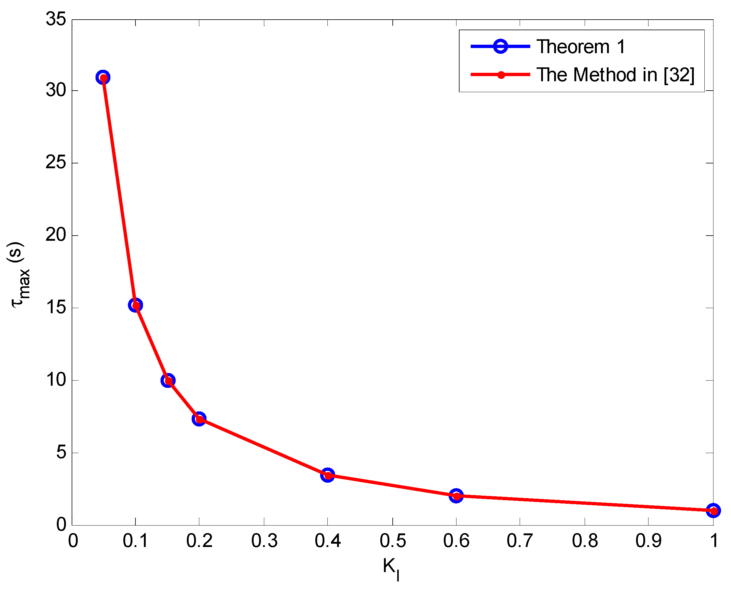
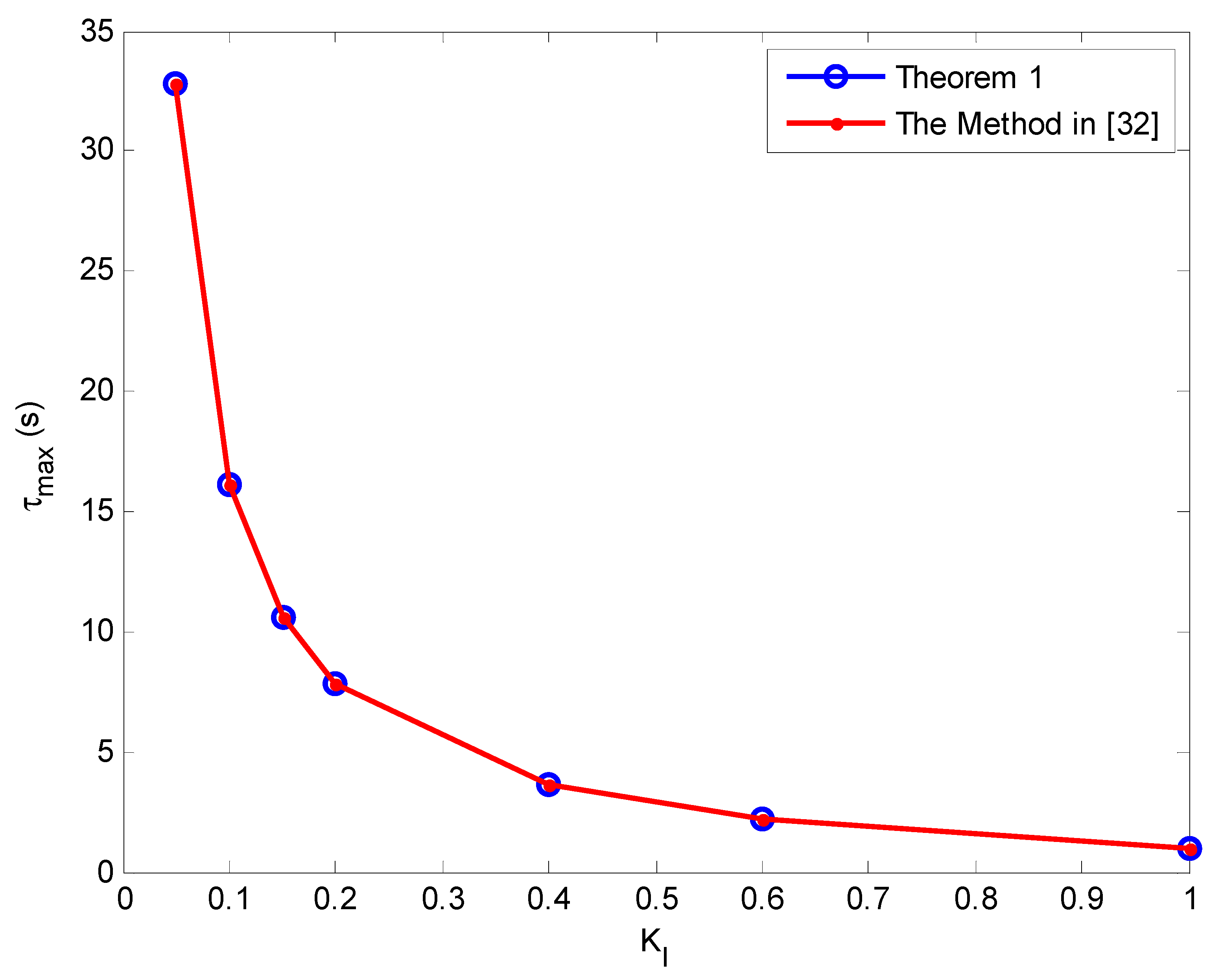
| 0 | Theorem 1 | 30.928 | 15.207 | 9.961 | 7.338 | 3.382 | 2.042 | 0.923 |
| [32] | 30.915 | 15.201 | 9.96 | 7.335 | 3.382 | 2.042 | 0.923 | |
| [18] | 30.853 | 15.172 | 9.942 | 7.323 | 3.377 | 2.04 | 0.922 | |
| [16] | 27.927 | 13.778 | 9.056 | 6.692 | 3.124 | 1.91 | 0.886 | |
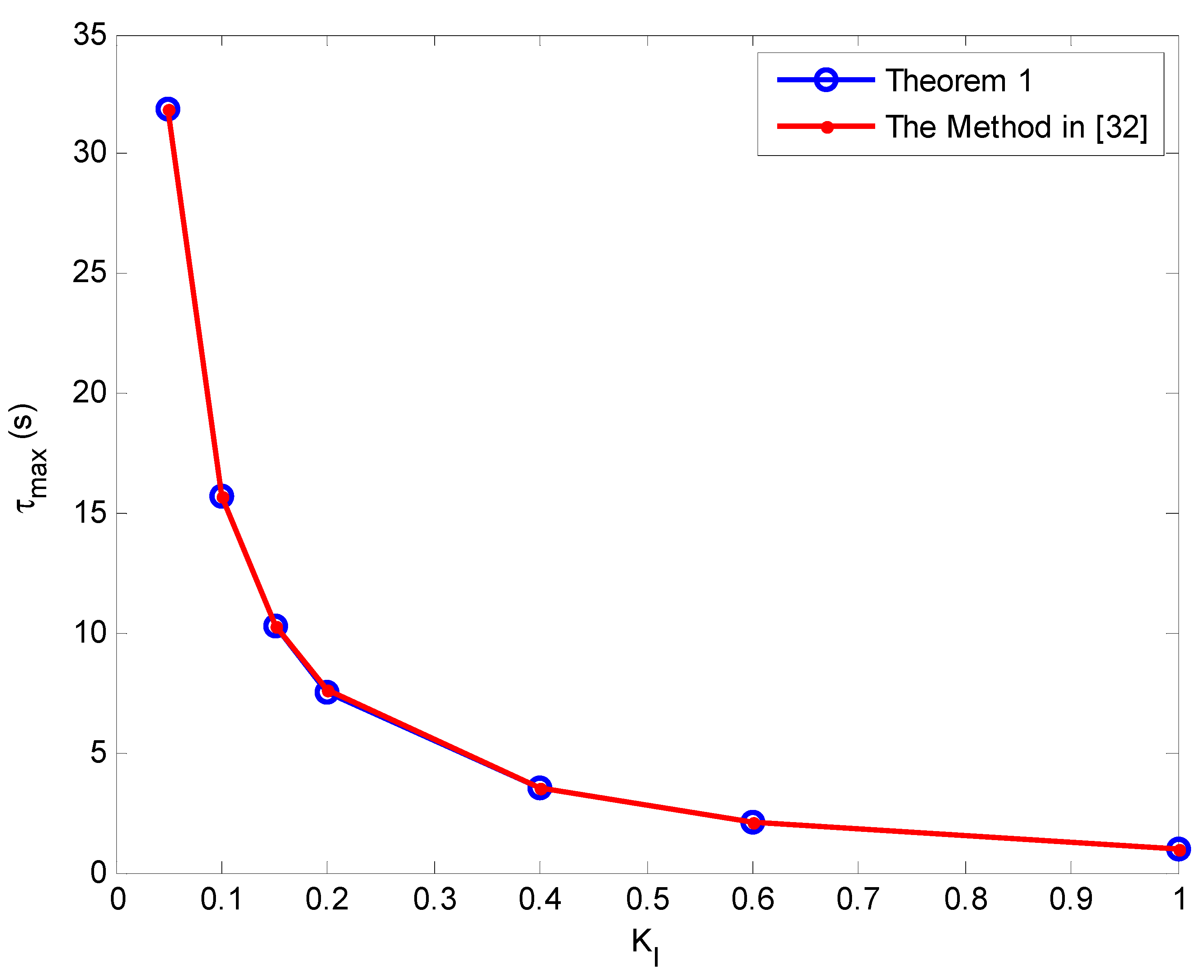
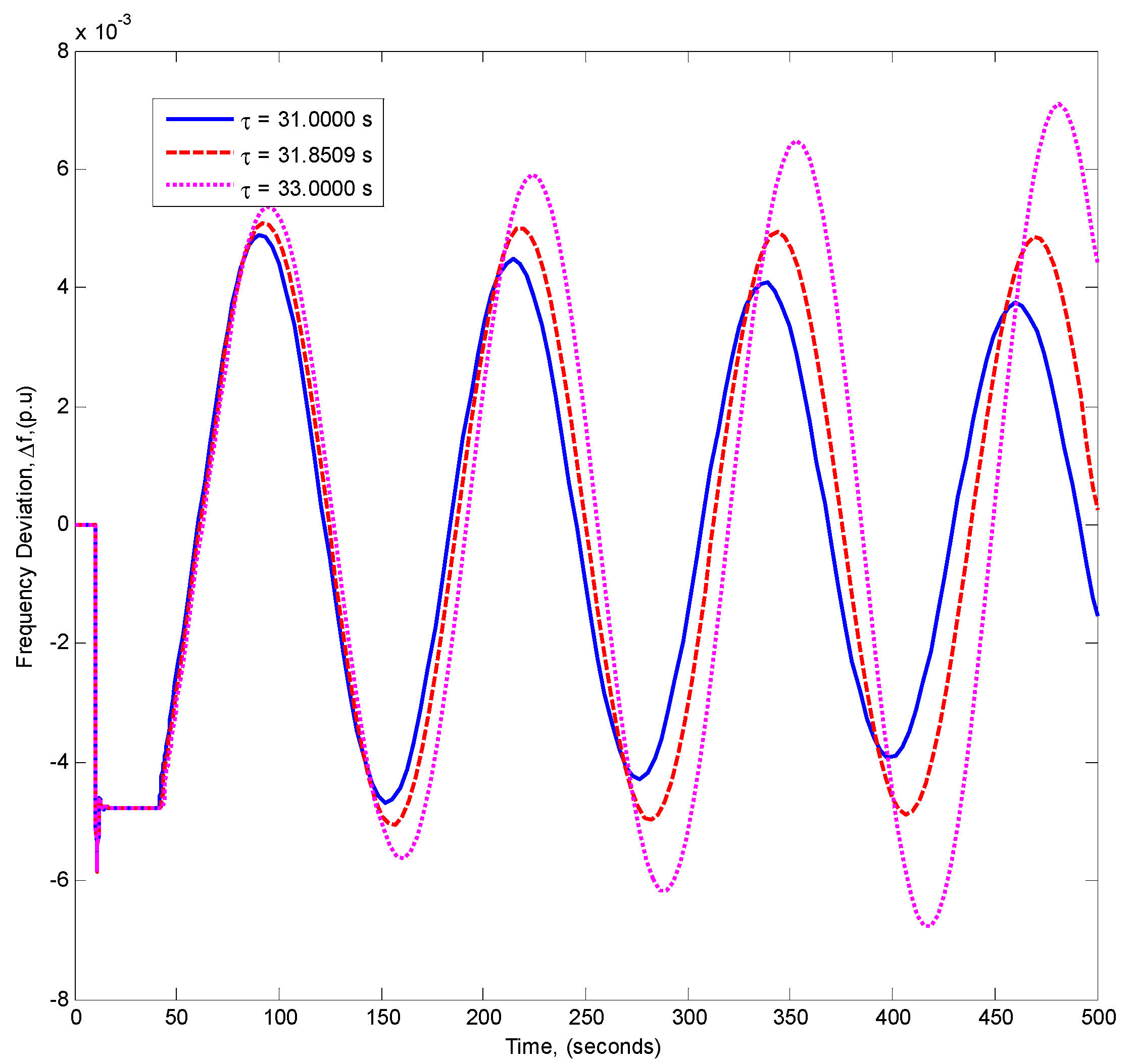
| 0.05 | Theorem 1 | 31.851 | 15.687 | 10.277 | 7.573 | 3.502 | 2.122 | 0.97 |
| [32] | 31.875 | 15.681 | 10.279 | 7.575 | 3.501 | 2.122 | 0.97 | |
| [18] | 31.498 | 15.647 | 10.258 | 7.561 | 3.496 | 2.119 | 0.969 | |
| [16] | 27.874 | 14.061 | 9.284 | 6.866 | 3.215 | 1.974 | 0.927 | |
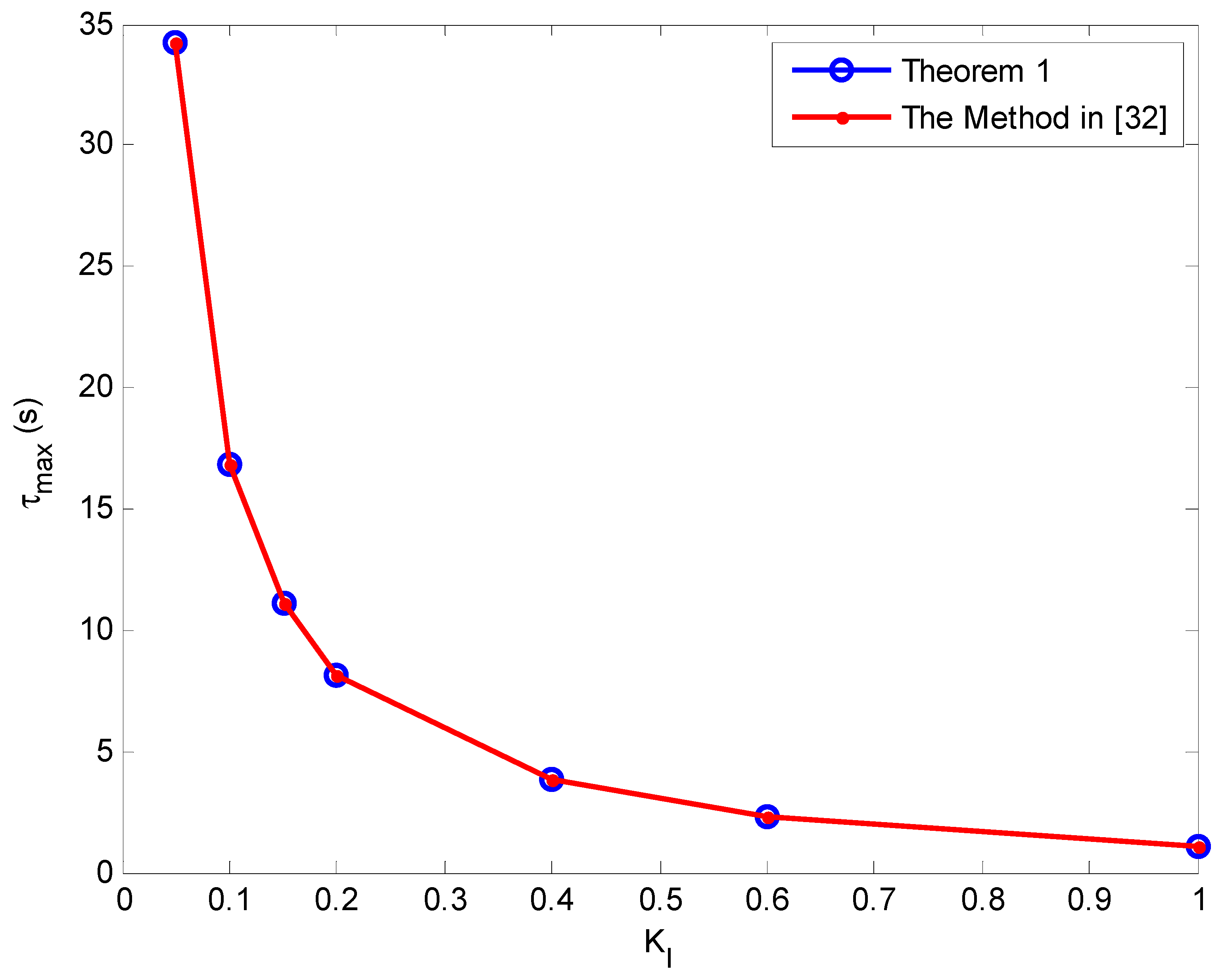
| 0.1 | Theorem 1 | 32.769 | 16.127 | 10.575 | 7.793 | 3.61 | 2.194 | 1.012 |
| [32] | 32.751 | 16.119 | 10.571 | 7.794 | 3.61 | 2.194 | 1.012 | |
| [18] | 30.415 | 15.765 | 10.547 | 7.777 | 3.604 | 2.191 | 1.011 | |
| [16] | 27.038 | 13.682 | 9.22 | 6.941 | 3.29 | 2.029 | 0.963 | |
| 0.2 | Theorem 1 | 34.198 | 16.86 | 11.06 | 8.16 | 3.792 | 2.313 | 1.079 |
| [32] | 34.226 | 16.856 | 11.062 | 8.162 | 3.792 | 2.313 | 1.079 | |
| [18] | 28.01 | 14.597 | 10.107 | 7.821 | 3.784 | 2.309 | 1.077 | |
| [16] | 25.114 | 12.76 | 8.617 | 6.535 | 3.32 | 2.108 | 1.016 | |
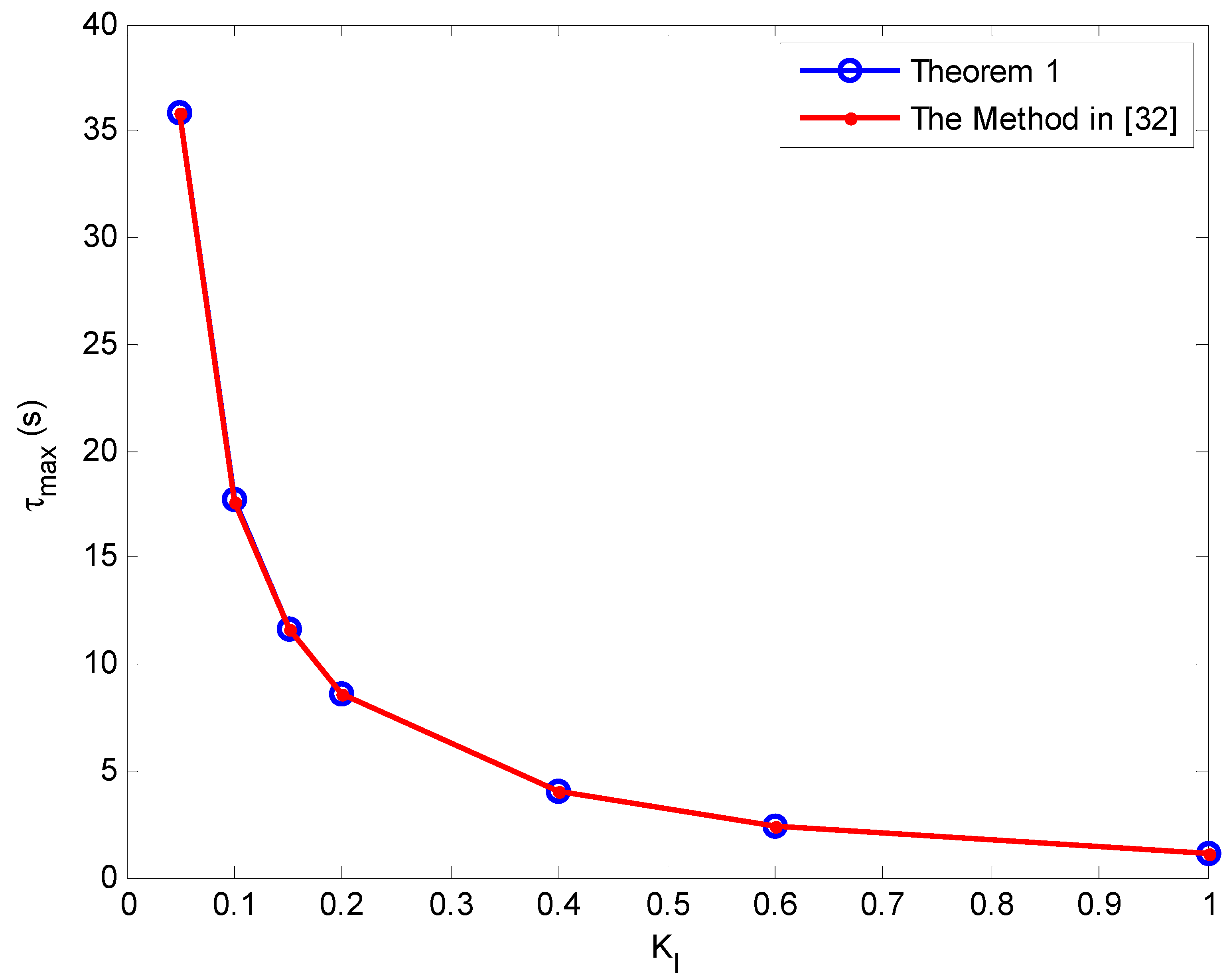
| 0.4 | Theorem 1 | 35.802 | 17.661 | 11.596 | 8.559 | 3.981 | 2.426 | 1.118 |
| [32] | 35.834 | 17.658 | 11.594 | 8.559 | 3.98 | 2.426 | 1.118 | |
| [18] | 22.457 | 11.835 | 8.287 | 6.505 | 3.718 | 2.419 | 1.116 | |
| [16] | 20.364 | 10.426 | 7.065 | 5.384 | 2.832 | 1.912 | 1.017 | |
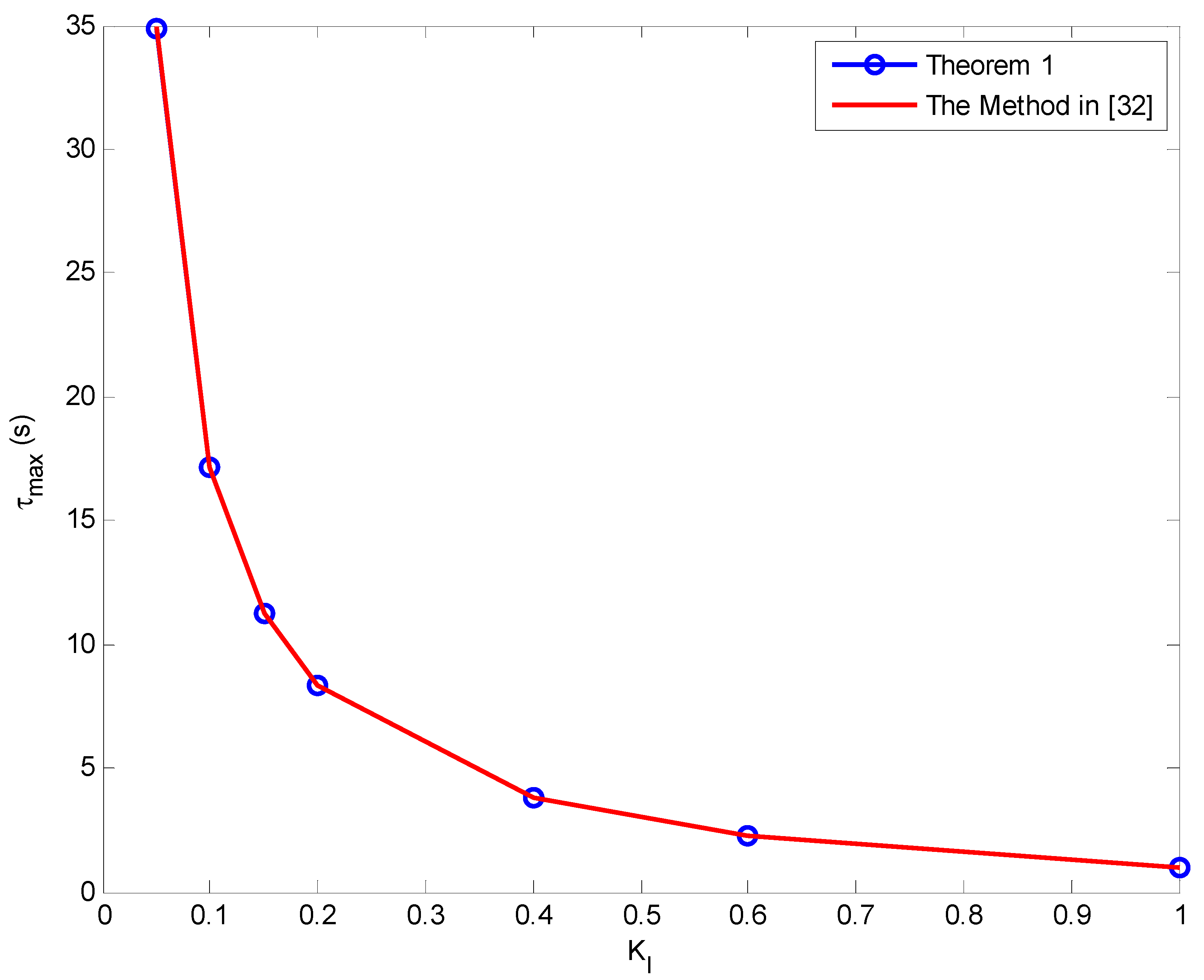
| 0.6 | Theorem 1 | 34.906 | 17.198 | 11.28 | 8.311 | 3.826 | 2.281 | 0.947 |
| [32] | 34.922 | 17.195 | 11.278 | 8.312 | 3.826 | 2.281 | 0.947 | |
| [18] | 16.033 | 8.624 | 6.209 | 4.997 | 3.038 | 2.178 | 0.964 | |
| [16] | 14.618 | 7.477 | 5.157 | 3.958 | 2.13 | 1.475 | 0.827 | |
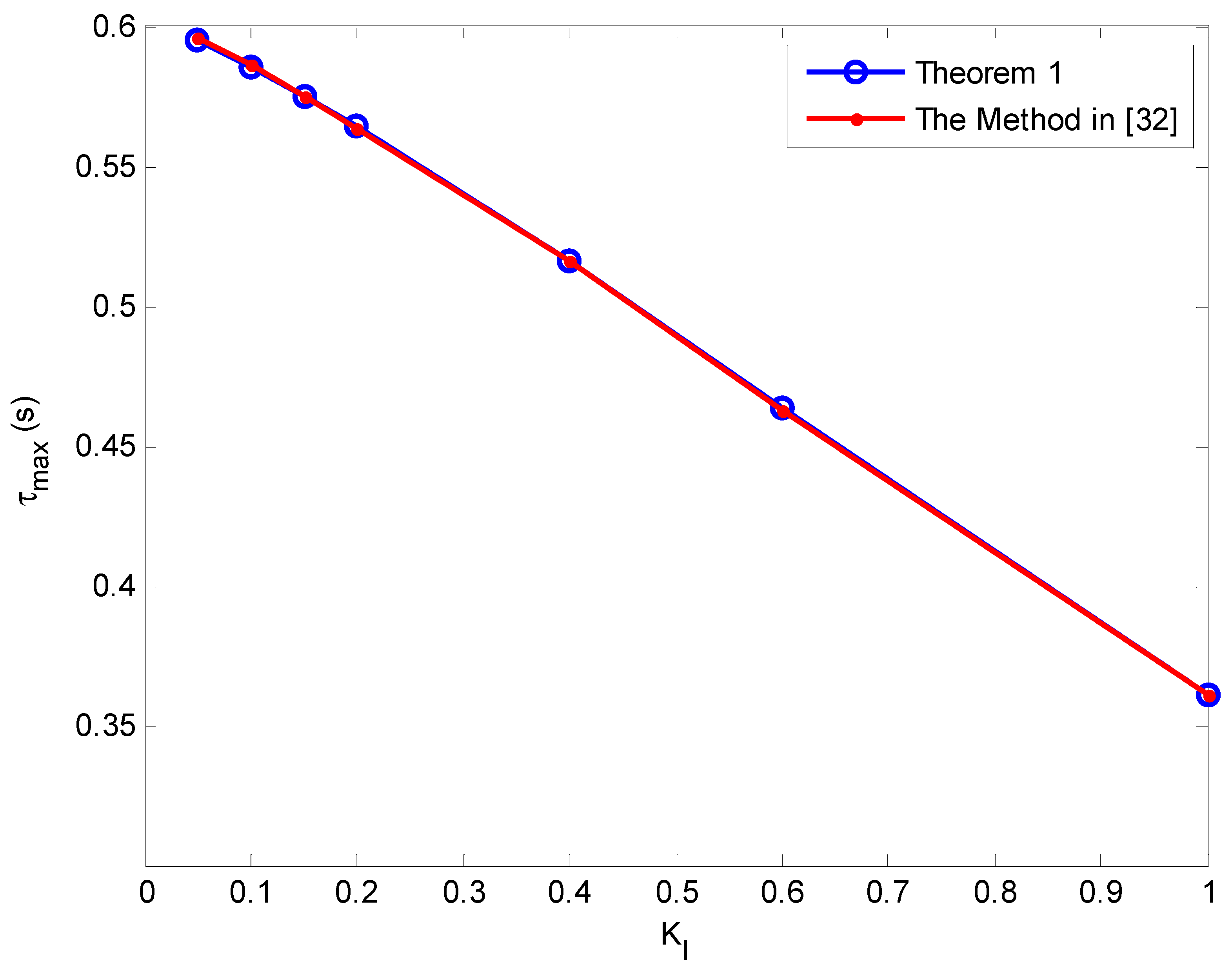
| 1 | Theorem 1 | 0.595 | 0.586 | 0.575 | 0.564 | 0.516 | 0.463 | 0.361 |
| [32] | 0.596 | 0.586 | 0.575 | 0.564 | 0.516 | 0.463 | 0.361 | |
| [18] | 0.594 | 0.584 | 0.574 | 0.563 | 0.515 | 0.463 | 0.36 | |
| [16] | 0.546 | 0.538 | 0.53 | 0.522 | 0.482 | 0.438 | 0.348 | |
| θ/rad | KI | ||||||
|---|---|---|---|---|---|---|---|
| KP | 0.05 | 0.1 | 0.15 | 0.2 | 0.4 | 0.6 | 1.0 |
| 0 | 1.546 | 1.521 | 1.496 | 1.471 | 1.368 | 1.257 | 0.989 |
| 0.05 | 1.596 | 1.571 | 1.546 | 1.521 | 1.418 | 1.307 | 1.041 |
| 0.1 | 1.646 | 1.621 | 1.596 | 1.571 | 1.468 | 1.358 | 1.092 |
| 0.2 | 1.747 | 1.722 | 1.696 | 1.671 | 1.567 | 1.456 | 1.187 |
| 0.4 | 1.956 | 1.929 | 1.902 | 1.875 | 1.765 | 1.647 | 1.349 |
| 0.6 | 2.184 | 2.153 | 2.123 | 2.092 | 1.968 | 1.828 | 1.419 |
| 1.0 | 1.435 | 1.413 | 1.390 | 1.365 | 1.262 | 1.152 | 0.934 |
| ω/(rad/s) | KI | ||||||
|---|---|---|---|---|---|---|---|
| KP | 0.05 | 0.1 | 0.15 | 0.2 | 0.4 | 0.6 | 1.0 |
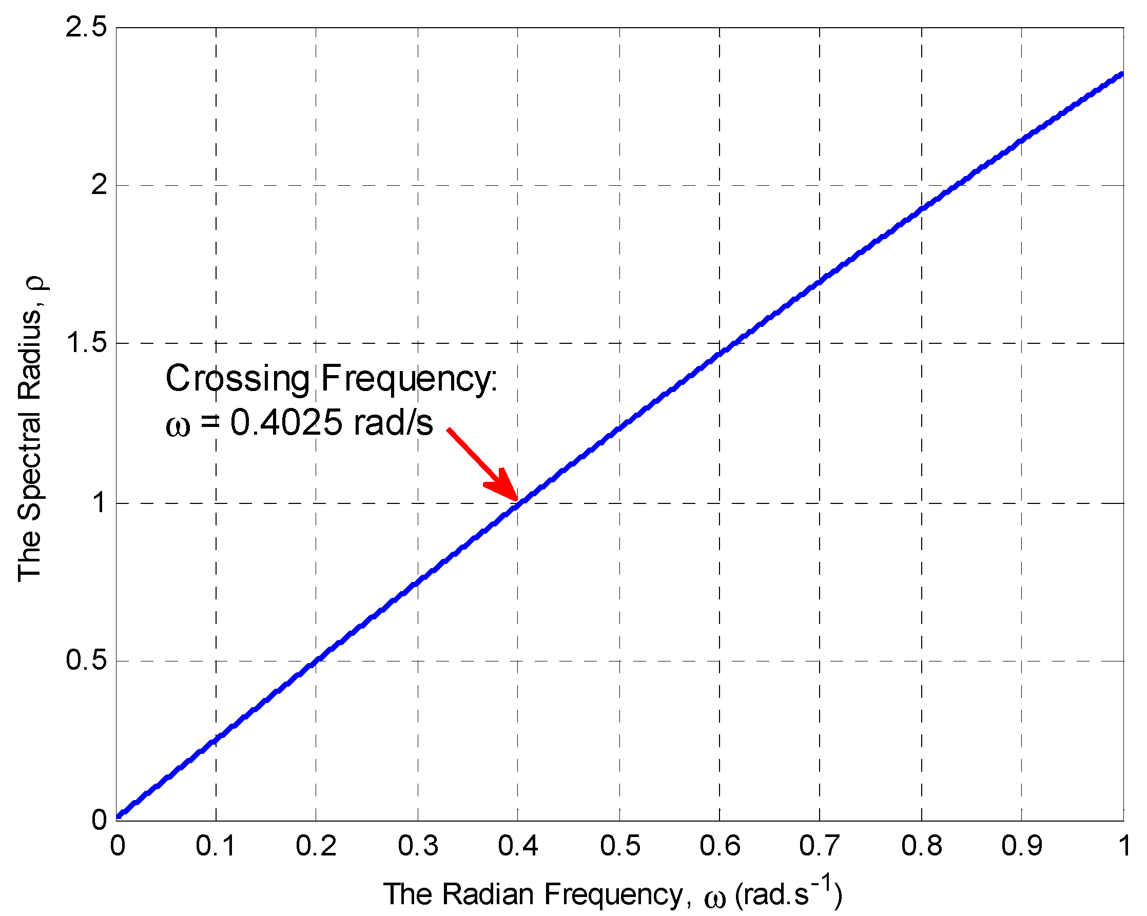
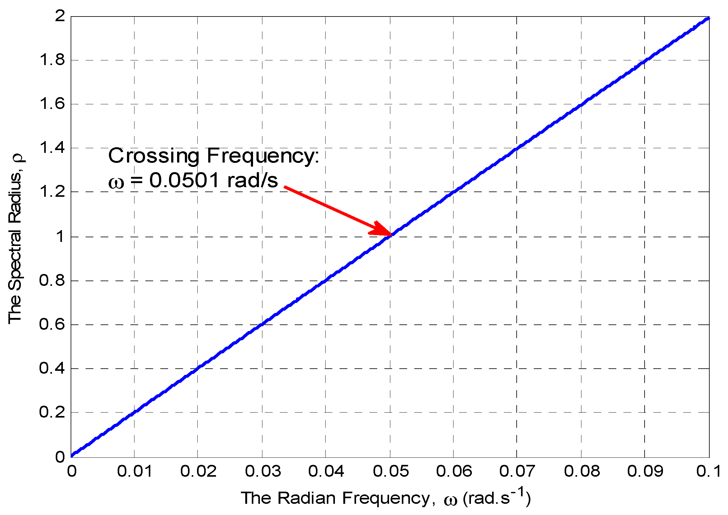
| 0 | 0.0500 | 0.1000 | 0.1502 | 0.2005 | 0.4045 | 0.6153 | 1.0714 |
| 0.05 | 0.0501 | 0.1002 | 0.1505 | 0.2009 | 0.4050 | 0.6161 | 1.0732 |
| 0.1 | 0.0502 | 0.1005 | 0.1509 | 0.2016 | 0.4067 | 0.6187 | 1.0784 |
| 0.2 | 0.0511 | 0.1021 | 0.1534 | 0.2048 | 0.4133 | 0.6295 | 1.1004 |
| 0.4 | 0.0546 | 0.1092 | 0.1640 | 0.2191 | 0.4434 | 0.6789 | 1.2065 |
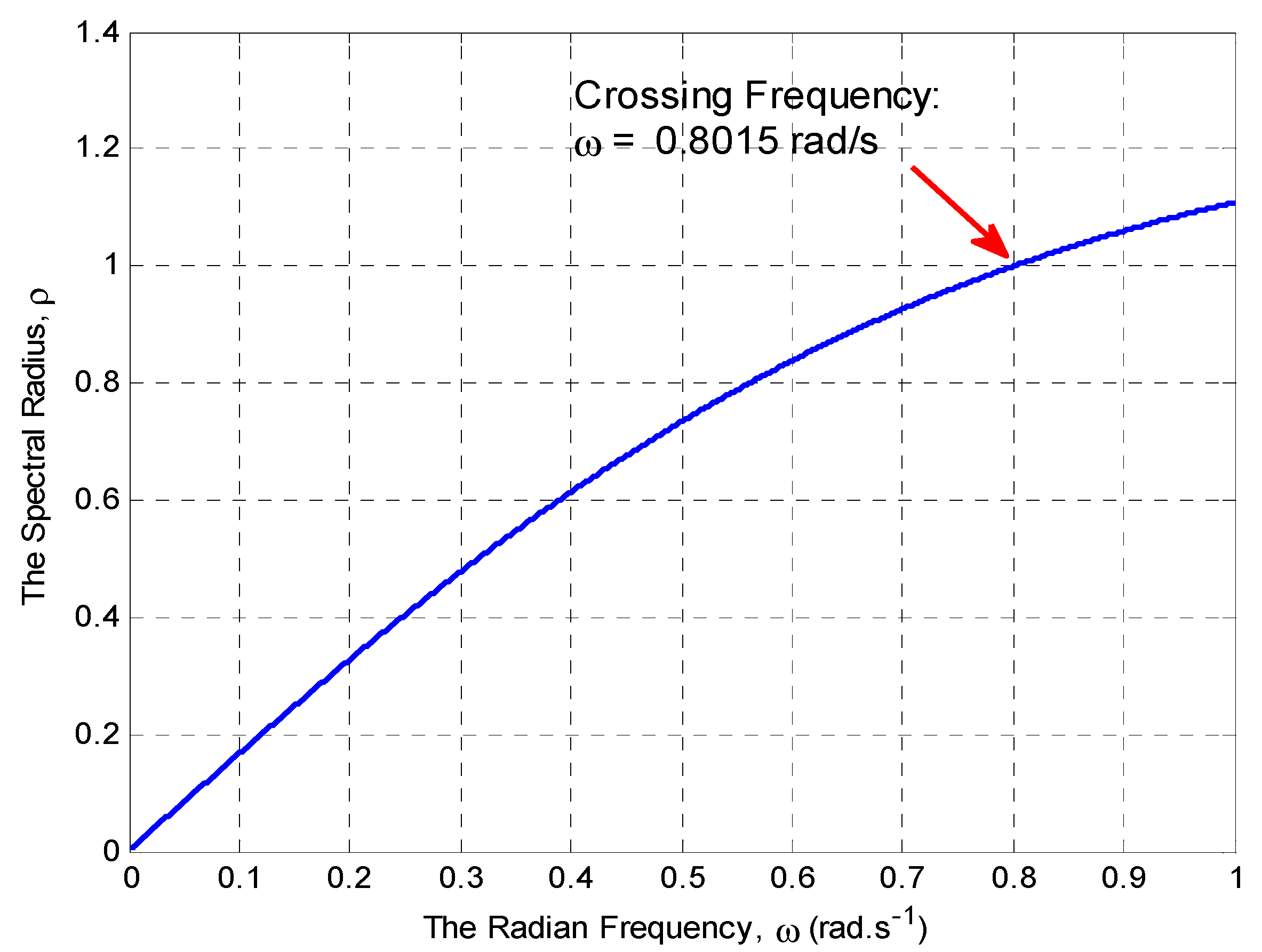
| 0.6 | 0.0626 | 0.1252 | 0.1882 | 0.2518 | 0.5143 | 0.8015 | 1.4981 |
| 1.0 | 2.4102 | 2.4120 | 2.4151 | 2.4193 | 2.4462 | 2.4861 | 2.5867 |
| KI | θ | ω | τd |
|---|---|---|---|
| 0.05 | 1.5460 | 0.0500 | 30.9283 |
| 0.1 | 1.5212 | 0.1000 | 15.2066 |
| 0.15 | 1.4963 | 0.1502 | 9.9614 |
| 0.2 | 1.4712 | 0.2005 | 7.3375 |
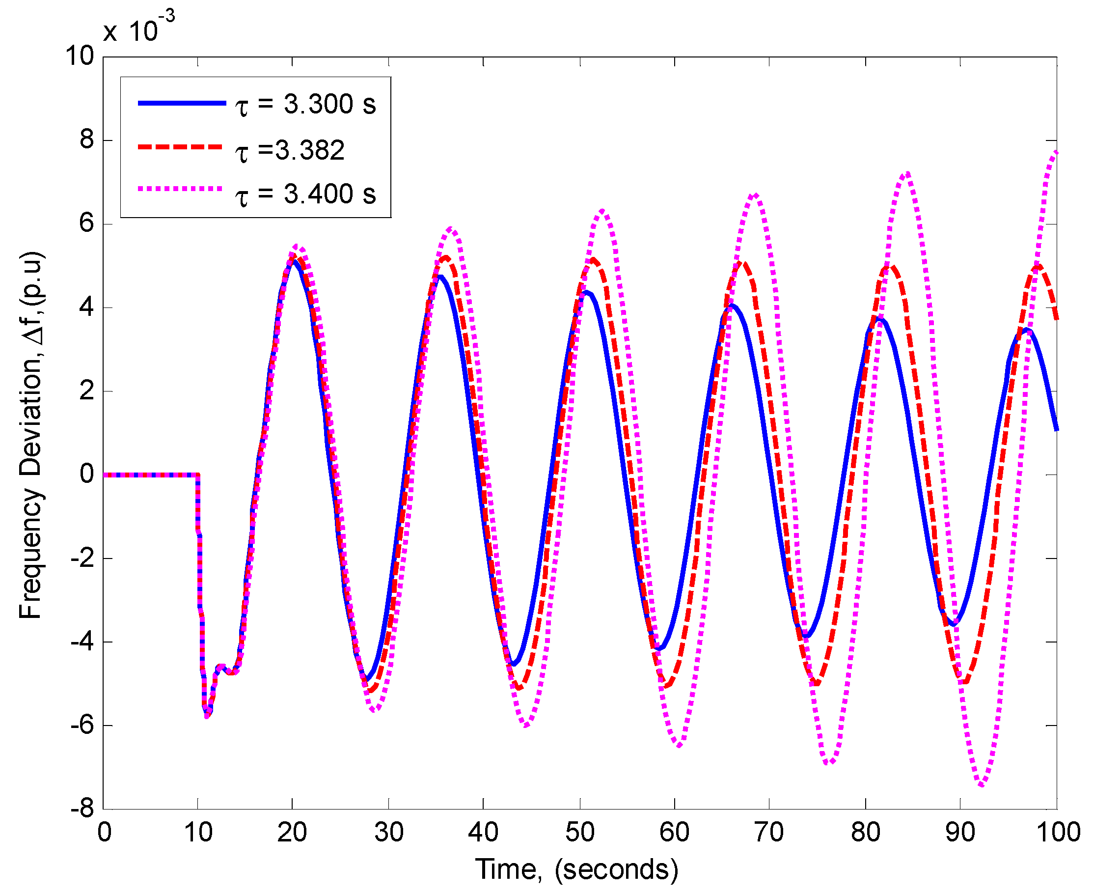
| 0.4 | 1.3678 | 0.4045 | 3.3816 |
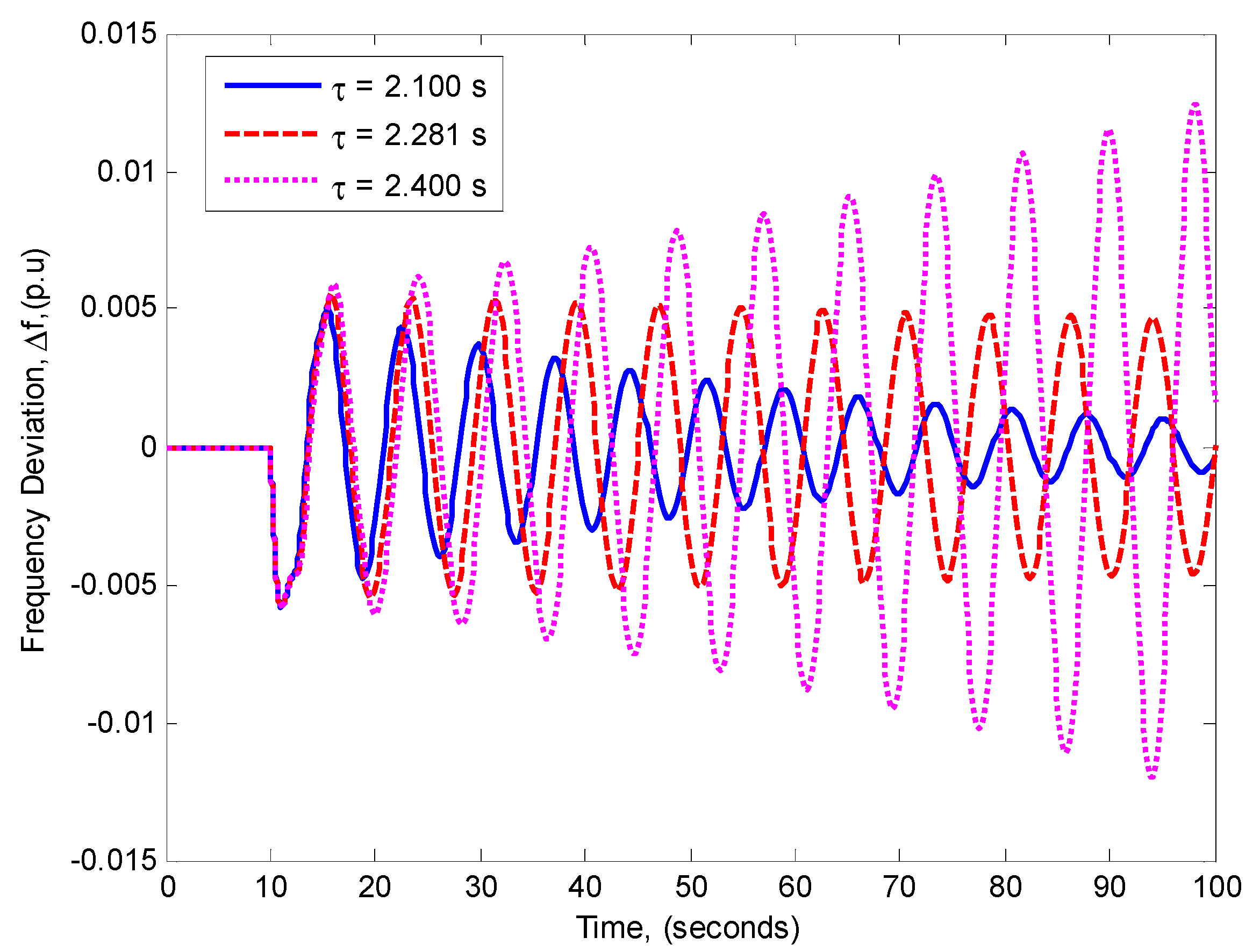
| 0.6 | 1.2566 | 0.6153 | 2.0422 |
| 1.0 | 0.9889 | 1.0714 | 0.9230 |
© 2018 by the authors. Licensee MDPI, Basel, Switzerland. This article is an open access article distributed under the terms and conditions of the Creative Commons Attribution (CC BY) license (http://creativecommons.org/licenses/by/4.0/).
Share and Cite
Khalil, A.; Swee Peng, A. A New Method for Computing the Delay Margin for the Stability of Load Frequency Control Systems. Energies 2018, 11, 3460. https://doi.org/10.3390/en11123460
Khalil A, Swee Peng A. A New Method for Computing the Delay Margin for the Stability of Load Frequency Control Systems. Energies. 2018; 11(12):3460. https://doi.org/10.3390/en11123460
Chicago/Turabian StyleKhalil, Ashraf, and Ang Swee Peng. 2018. "A New Method for Computing the Delay Margin for the Stability of Load Frequency Control Systems" Energies 11, no. 12: 3460. https://doi.org/10.3390/en11123460
APA StyleKhalil, A., & Swee Peng, A. (2018). A New Method for Computing the Delay Margin for the Stability of Load Frequency Control Systems. Energies, 11(12), 3460. https://doi.org/10.3390/en11123460