Article

Transient Modelling of Rotating and Stationary Cylindrical Heat Pipes: An Engineering Model

1
Process & Energy Department, Faculty of Mechanical, Maritime and Materials Engineering, Delft University of Technology, 2628 CB Delft, The Netherlands
2
Research & Development, Tata Steel, 1951 JZ Velsen-Noord, The Netherlands
*
Author to whom correspondence should be addressed.
Energies 2018, 11(12), 3458; https://doi.org/10.3390/en11123458
Submission received: 14 November 2018 / Revised: 28 November 2018 / Accepted: 6 December 2018 / Published: 10 December 2018
(This article belongs to the Section J: Thermal Management)

Abstract

:
Rotating wickless and stationary capillary cylindrical heat pipes are widely used heat transfer devices. Transient behavior of such heat pipes has been investigated numerically with computational fluid dynamics and lumped parameter models. In this paper, the advantages of both methods are combined into a novel engineering model that is low in computational cost but still accurate and rich in the details it provides. The model describes the interior dynamics of the heat pipe with a 2D representation of a cylindrical heat pipe. Liquid and vapor volumes are coarsely meshed in the axial direction. The cells are allowed to change in size in the radial direction during simulation. This allows for tracking the liquid/vapor interface without having to implement fine meshing. The model includes the equations for mass, momentum and energy and is applicable to both rotating and stationary heat pipes. The predictions of the model are validated with other experimental, numerical, and analytical works having an average deviation of less than 4%. The effects of various parameters on the system are explored. The presented model is suitable for the simulation of heat pipe systems in which both the level of detail and the computational cost are crucial factors.

1. Introduction

Heat pipes are efficient heat transfer devices that make use of a working fluid acting as an energy carrier. Typical heat pipes are composed of three sections: evaporator, adiabatic section, and condenser. The heat received at the evaporator of the heat pipe causes the liquid to evaporate. The vapor then flows to the condenser end of the heat pipe. The heat extraction causes the vapor to condense at the condenser of the heat pipe providing a pressure decrease that further promotes the transport of vapor. Finally, the liquid is transported from the condenser back to the evaporator [1,2,3]. Various types of heat pipes deal with the transport of the liquid back to the evaporator in different ways. Stationary capillary heat pipes (SCHP) with a wick structure make use of the capillary force to drive the liquid [4], whereas rotating heat pipes (RHP) employ centrifugal force [5].
Heat pipes are widely used in thermal management systems due to their reliability and effectiveness. SCHPs are used in the cooling of electronics, in space applications as well as in thermal energy storage systems [1]. Various studies have been carried out to investigate their performance in such applications [6,7,8,9,10,11,12]. On the other hand, RHPs are mainly used in applications such as the cooling of drill tips [13], cooling of rotating electrical machines [14,15,16] and heating/cooling of metal strips [17].
In order to predict the transient behavior of heat pipes and to improve their designs, various numerical methods have been developed. For the dynamic modelling of SCHPs, these methods range from thermal network analysis to detailed computational fluid dynamics (CFD). Zuo et al. [3] described the heat pipe as a collection of lumped masses with specific thermal resistances. This model allows for the simplification of the governing equations to first-order linear ordinary differential equations (ODEs). The dynamic behavior of a flat plate heat pipe has been described by Xuan et al. [18], who solved the transient conduction equation for the wall and the wick region, whereas a lumped model is used for the vapor phase. Another lumped parameter approach has been adapted by Ferrandi et al. [19], which also accounts for liquid and vapor flow and storage. In their work, the governing equations for fluids are solved by assuming that each phase is held in two tanks (evaporator and condenser) with a communication path connecting them. Wits et al. [20] used a control volume element approach to model the transient behavior of a flat miniature heat pipe. In this control volume method, the liquid and the vapor at the evaporator and the condenser are separately lumped into two control volumes and the governing equations are solved. Tournier et al. [21] developed a two-dimensional transient model in which the energy and momentum discontinuities at the liquid/vapor interface are incorporated. In this work, special attention is paid to the prediction of liquid pooling and the curvature of the liquid meniscus. Solomon et al. [22] presented a transient CFD model where Navier–Stokes equations are solved for a very fine mesh with the assumption of a laminar and incompressible two-dimensional flow.
For RHPs, steady-state modelling has been extensively addressed [23,24,25], with recent studies focusing on the use of nanofluids [26,27]. On the other hand, transient modelling studies are scarce. A detailed dynamic model is presented by Harley et al. [28], which solved the continuity, momentum, and energy equations for an axisymmetric geometry on a fixed grid. In this model, the set of highly non-linear equations are solved using the SIMPLE algorithm. Baker et al. [29] have solved the Navier–Stokes equations and the energy equation using the volume of fluid (VOF) model to predict the liquid-vapor interface. A more recent study by Lian et al. [30] also describes the transient behavior of the heat pipe with Navier–Stokes equations and VOF using a novel phase-change model. For all these studies, the modelled RHPs have a conical shape at the condenser or throughout. This conical shape inside an RHP is commonly referred to as a taper and it increases the efficiency of the heat pipe by promoting lower liquid thickness at the condenser. The presented work, on the other hand, focuses on a cylindrical geometry because many applications necessitate the use of cylindrical RHPs due to cost of manufacturing or functional requirements.
In the presented work, a transient heat pipe model that is applicable to cylindrical SCHPs and RHPs is introduced. The main objective of the model is to provide sufficient details about the interior dynamics of the heat pipes without experiencing long computational times. It is important to avoid the loss of details of lumped parameter models, in particular for the modelling of SCHPs, where it is a common practice. Avoiding long computational times, on the other hand, is especially crucial for the modelling attempts towards RHPs, which were solely based on CFD so far.
In order to achieve these objectives, the 2D axisymmetric geometry of the heat pipe is coarsely meshed in the axial direction for the wall, the liquid and the vapor. The liquid and the vapor cells are allowed to change size in the radial direction during the simulation. In this way, there is no need for fine meshing especially near the liquid/vapor interface. Transient mass, momentum and energy equations are solved for each cell.
With this approach, heat pipes can be simulated with relatively low computational cost and still describe dynamics in detail. This is especially advantageous for design calculations and for the dynamic modelling of large systems involving one or multiple heat pipes.

2. Model Description
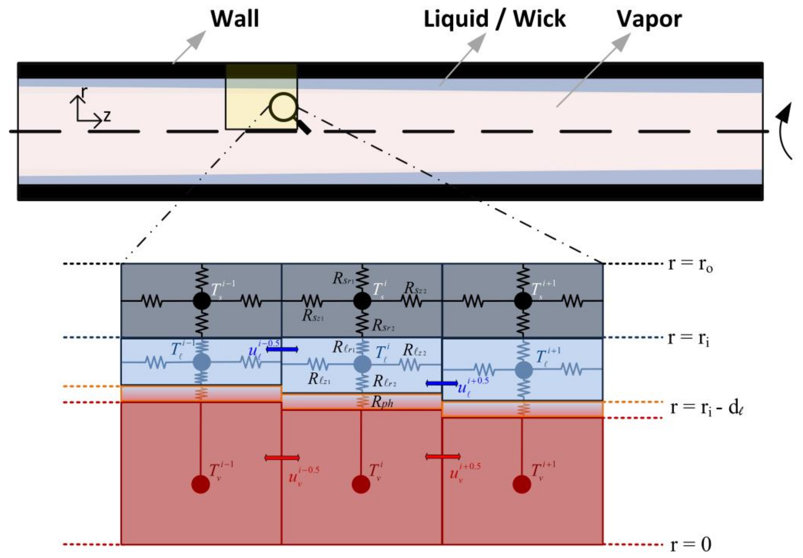
2.1. Model Geometry

The model geometry is a 2D representation of a cylindrical heat pipe, making use of its symmetry along the angular direction. The three main components of the model are the heat pipe wall, the liquid, and the vapor, each modelled as a single lumped mass in the radial direction. They are all axially meshed to a desired number of cells, irrespective of the heat pipe section they belong to. All of the wall cells are governed by the same set of equations. The same is valid for all liquid cells and all vapor cells. The connection of a group of cells is shown in Figure 1.
Each node in Figure 1 is a lump mass characterized by a unique thermodynamic state. The resistances are associated with thermal conduction through the material and the phase change. As can be seen in the figure, the mesh is staggered such that the temperatures and pressures are located at cell centers, whereas velocities are located at cell faces. The liquid and the vapor mesh can grow and shrink in the radial direction. In this way, the location of the interface for an axial location can change in time and liquid head can be incorporated in the model. The architecture of the nodes and their connections allow the same equations to be used throughout the whole heat pipe.

2.2. Model Assumptions

In order to create a practical, applicable and yet sufficiently detailed model of the heat pipe functioning, several simplifications and assumptions are made. These simplifications and assumptions follow out of the selected model geometry. They are itemized below with the relevant references from similar studies when applicable:
  • An axisymmetric geometry is chosen, requiring the omission of gravity, which is unidirectional in reality.
  • A one-dimensional approach is taken for the flow of liquid and vapor.
  • The heat input and output to the lumped masses through the resistances are linearly approximated [3,28].
  • The vapor is treated as an ideal gas [22,28].
  • The liquid and the vapor are incompressible [28,31].
  • Thermal expansion of the heat pipe container and the wick is neglected.
  • The liquid layer thickness is much smaller than the radius of the heat pipe [24,28].
  • The dynamics of the vapor is much faster than the dynamics of the other components [3]. Therefore, the vapor is assumed to be always saturated, taking into account the mass flows of the phase change and its associated latent heat.
  • The pressure drop of the vapor is much smaller than the pressure drop of the liquid along the heat pipe [21,24,32].
  • For rotating heat pipes without a wick structure, the thermal conduction through the liquid in the axial direction is neglected [23,24,25].
  • For the liquid component of the rotating heat pipes without a wick structure, the heat transfer in the radial direction is taken to be dominant over the heat transfer in the axial direction [24,25,28].

2.3. Governing Physics

Following the model geometry (Figure 1) and the simplifications (Section 2.2), the governing equations for the different components are formulated.
Firstly, the thermal resistances in the radial and axial directions shown in Figure 1 are defined according to Equations (1) and (2):
R r a d i a l = ln ( 𝓇 o / 𝓇 i ) 2 π   k   Δ z
R a x i a l = Δ z k   A
where R r a d i a l and R a x i a l are the thermal resistances at the radial and axial directions respectively, 𝓇 o and 𝓇 i are the outer and inner radii of the given resistance respectively, k is the thermal conductivity of the component, Δ z is the length of the resistance in the axial direction and A is the cross-sectional area of the cell in the axial direction. In case of SCHP, the effective thermal conductivity of the liquid/wick is calculated using Equation (3) [22].
k e f f = k [ ( k + k w ) ( 1 ε ) ( k k w ) ( k + k w ) + ( 1 ε ) ( k k w ) ]
where ε is the porosity of the wick and the subscripts and w represent liquid and wick, respectively.

2.3.1. Wall Component

Following the definition of the thermal resistances, the transient energy equation for a wall component is defined as in Equation (4) in its discretized form in space.
m s i d ( c p s i T s i ) d t = Q ˙ + T i T s i R s r 2 i + R r 1 i + T s i 1 T s i R s z 2 i 1 + R s z 1 i + T s i + 1 T s i R s z 1 i + 1 + R s z 2 i
where c p is the specific heat, m is the mass of the node, T is the temperature, t is the time, Q ˙ is the external heat flow to/from the node, the subscript s represents the solid wall and the superscript i points to the index of the node. The relevant thermal resistances are shown in Figure 1. This equation shows that the change in the energy content of a wall component depends on the external heat flow to/from the node as well as the heat conduction through it.

2.3.2. Liquid Component

For the liquid component, the governing equations for mass, momentum and energy are simultaneously solved. All these equations are presented in their discretized forms in space. The continuity equation for a given liquid node is described in Equation (5).
ε   d ( ρ i V l i ) d t = ε   ρ i 0.5 A i 0.5 u i 0.5 ε   ρ i + 0.5 A i + 0.5 u i + 0.5 m ˙ p h i
where ρ is the density, V is the volume, u is the velocity and m ˙ p h is the phase change rate. Porosity for a wickless RHP is taken as 1 ( ε = 1 ). Upwind scheme can be used for the computation of properties at the cell interfaces.
The phase change rate m ˙ p h and the cross-sectional area of the liquid node A l are defined with Equations (6) and (7).
m ˙ p h = T i T v i ( R r 2 i + R p h i )   H f g
A l i = π ( r i 2 ( r i d i ) 2 )
where H f g is the latent heat, r i is the inner radius of the heat pipe, d is the thickness of the liquid layer and the subscript v represents vapor. The thermal resistances are illustrated in Figure 1. The thermal resistance associated with phase change, R p h , is often neglected as it is orders of magnitude lower than the other thermal resistances shown in Figure 1 [2]. However, it should be accounted for in the simulation of heat pipes filled with alkali metal [33].
The liquid momentum equation is defined with Equation (8).
d ( ρ i + 0.5 u i + 0.5 ) d t = Δ p Δ z ρ i + 1 ( u i + 1 ) 2 Δ z + ρ i ( u i ) 2 Δ z + γ
where Δ z is the distance between the adjacent node centers, Δ p is the pressure difference between adjacent nodes and γ is the viscous term of the momentum equation. The second and the third terms on the right-hand side are the convective terms. In order to calculate the liquid velocities at the cell centers (see the convective terms), Equation (9) is used.
u i = u i 0.5 + u i + 0.5 2
The pressure term and the viscous term are evaluated differently for SCHPs and RHPs. For an SCHP, the pressure term is calculated using Equation (10).
Δ p S C H P = f 2   σ r c  
where 2   σ / r c is the maximum capillary pressure [34] with σ being the surface tension and r c being the capillary radius. f is a correction coefficient accounting for the change in contact angle fluid-wick between adjacent nodes. This change is commonly approximated as the difference in the liquid fill ratio of the wick between adjacent nodes [19,20].
The viscous term for an SCHP is calculated with the well-established equation for laminar flows [2].
γ SCHP = μ K ε   u
where μ is the viscosity and K is the wick permeability.
For the rotating heat pipe, on the other hand, the pressure term is calculated using Equation (12).
Δ p R H P = ( d i + 1 ρ i + 1 d i ρ i )   ω 2   r i
where ω is the rotational speed. It should be noted that in the studies concerning RHPs with a taper, the slope of the liquid film is often assumed to be much lower than the taper angle [23,28]. Therefore, the hydrostatic pressure gradient is neglected. In a cylindrical RHP however, it is crucial to account for the slope of the liquid film as it is the main driving force for the liquid flow from the condenser to the evaporator.
The calculation of the viscous term is not as straightforward as it is for the SCHP. In order to calculate the viscous term for the liquid flow, the axial velocity profile throughout the liquid film should be known. However, in the model only the average velocity for the liquid is calculated. Since the liquid velocity at an axial location can be defined as a second order polynomial in the radial coordinate [28,35], the velocity profile is approximated using a quadratic equation.
u ( r ) = C 1 r 2 + C 2 r + C 3
With three unknowns ( C 1 , C 2 and C 3 ), one needs three equations and/or boundary conditions to solve the velocity profile. The velocity profile is solved using the following equations.
r = r i     u = 0
r = r i d     u r = 0
u = 0 2 π r i d r i u l . r . d Φ . d r π ( r i 2 ( r i d ) 2 )
where the first equation is the no-slip boundary condition at the inner wall [23,24,25], the second equation is the negligible shear stress boundary condition at the liquid/vapor interface [24,36] and the third equation describes the average velocity as the velocity profile integrated over the liquid film divided by the cross-sectional area.
Once the velocity profile is known, the viscous term is calculated by integrating the expression in Equation (15) over the control volume of the relevant node and then dividing it by the node volume.
γ = C V μ ( 1 r r ( r u r ) ) V
The resulting expression for the viscous term is found as shown in Equation (16).
γ RHP = μ ( 4   C 1 r i 2 + 2   C 2 r i 4   C 1 ( r i d ) 2 2   C 2 ( r i d ) ) ( r i 2 ( r i d ) 2 )
Finally, the energy equation for the liquid is described with Equation (17).
ρ i V i ε   d ( c p i   T i ) d t + [ m w i   d ( c p w i   T i ) d t ] = T s i T i R s r 2 i + R r 1 i + T v i T i R p h i + R r 2 i + [ T i 1 T i R z 2 i 1 + R z 1 i + T i + 1 T i R z 1 i + 1 + R z 2 i ]
where the terms in brackets are only applicable to the SCHP with a wick structure. Porosity for the wickless RHP is taken as 1. The relevant resistances are shown in Figure 1.
For the evaporator section of an RHP, the liquid thermal resistance needs to be calculated by taking natural convection into consideration alongside thermal conduction wherever applicable. This can be done with the mixed convection evaporator model described by Song et al. [37,38] and Bertossi et al. [24] when the corresponding Rayleigh number exceeds a value of 400.

2.3.3. Vapor Component

Similar to the liquid component, the governing equations for the vapor component are the continuity, momentum, and energy equations. The continuity equation for a vapor node is presented in Equation (18). Together with Equation (5) where the continuity equation for a liquid node is defined, the total mass inside the heat pipe is conserved.
d ( ρ v i V v i ) d t = ρ v i 0.5 A v i 0.5 u v i 0.5 ρ v i + 0.5 A v i + 0.5 u v i + 0.5 + m ˙ p h i
The vapor momentum equation is described with Equation (19).
d ( ρ v i + 0.5 u v i + 0.5 ) d t = Δ p v Δ z ρ v i + 1 ( u v i + 1 ) 2 Δ z + ρ v i ( u v i ) 2 Δ z + γ v
where Δ p v is the vapor pressure difference between adjacent nodes. It is computed with Equation (20) through the use of Antoine equation for the calculation of vapor pressures.
Δ p v = 10 A B T v i + 1 + C 10 A B T i v + C
where A , B and C are Antoine equation constants.
Similar to the momentum equation of a liquid node, the second and the third terms on the right-hand side describe the convective terms. The viscous term is calculated in a way similar to the one in liquid without a wick structure. The velocity profile throughout the vapor core is represented with a second order polynomial as shown in Equation (21).
u v ( r ) = C 4 r 2 + C 5 r + C 6
For three unknowns ( C 4 , C 5 and C 6 ), three equations/boundary conditions are described.
r = 0     u v r = 0
r = r i d     u v = u
u v = 0 2 π 0 r i d l u v · r · d Φ · d r π ( r i d ) 2
where the first equation is the symmetry condition at the heat pipe center, the second equation is the no-slip boundary condition at the liquid/vapor interface [21,28] and the third equation describes the average velocity of the vapor. As in the viscous term calculation for liquid, the viscous term for vapor can be found by integrating the expression in Equation (15) over the control volume of the relevant node and then dividing it by the node volume. In this way, the viscous term for vapor flow is found as shown in Equation (23).
γ v = μ v ( 4   C 4 ( r i d ) 2 + 2   C 5   ( r i d ) ) ( r i d ) 2
Following the assumption of much faster vapor dynamics compared to other components, the vapor energy equation is calculated with the ideal gas law as shown in Equation (24).
p v i T v i = ρ v i g M
where g is the universal gas constant and M is the molecular weight of the fluid.

2.4. Boundary Conditions

The boundary conditions at the outer wall surface can be either of Type-II or Type-III.
r = r o     k d T d r = Q ˙       | |       k d T d r = 0       | |       k d T d r = ( h c o n v + h r a d ) [ T T w r o ]  
where r o is the outer radius of the heat pipe, Q ˙ is the heat flux, h c o n v is the convective heat transfer coefficient, h r a d is the linearized radiative heat transfer coefficient and finally T is the ambient temperature.
The boundary conditions applied to the end caps of the heat pipe are:
  z = 0     z = L     u = u v = 0             d T d z = 0
where L is the heat pipe length. The boundary condition at the symmetry line is:
r = 0     d T d r = 0
Additionally, the boundary conditions described in Equations (14) and (22) for the calculation of the viscous terms apply.

2.5. Numerical Solution

The governing equations are comprised of first-order ODEs and algebraic equations. This is a stiff problem, especially due the fast dynamics of the vapor compared to other components. Therefore, the system of equations is solved implicitly with the “MATLAB ode15i” function.
The mesh size in the axial direction can be changed according to the level of detail requested from the model. The accuracy deteriorates at a low number of computational cells especially when the liquid height is non-linear along the heat pipe length. This is usually the case when the fill ratio is very low, the heat flux is high and the heat pipe is long.

3. Results and Discussion

The model presented in the previous section is validated for SCHP and RHP. For SCHP, the validation is made for a transient case where the predictions are compared to the results from an experimental and a numerical work. For RHP, the predictions at steady-state are compared to the outcomes of an experimental work as well as to the steady-state analytical and numerical simulations. In this way, the validity of the developed model is tested for different types of heat pipes at different conditions. After the validations, the computational efficiency of the model is investigated. Finally, the effect of operating temperature on vapor dynamics and the effect of rotational speed on liquid height distribution are studied.

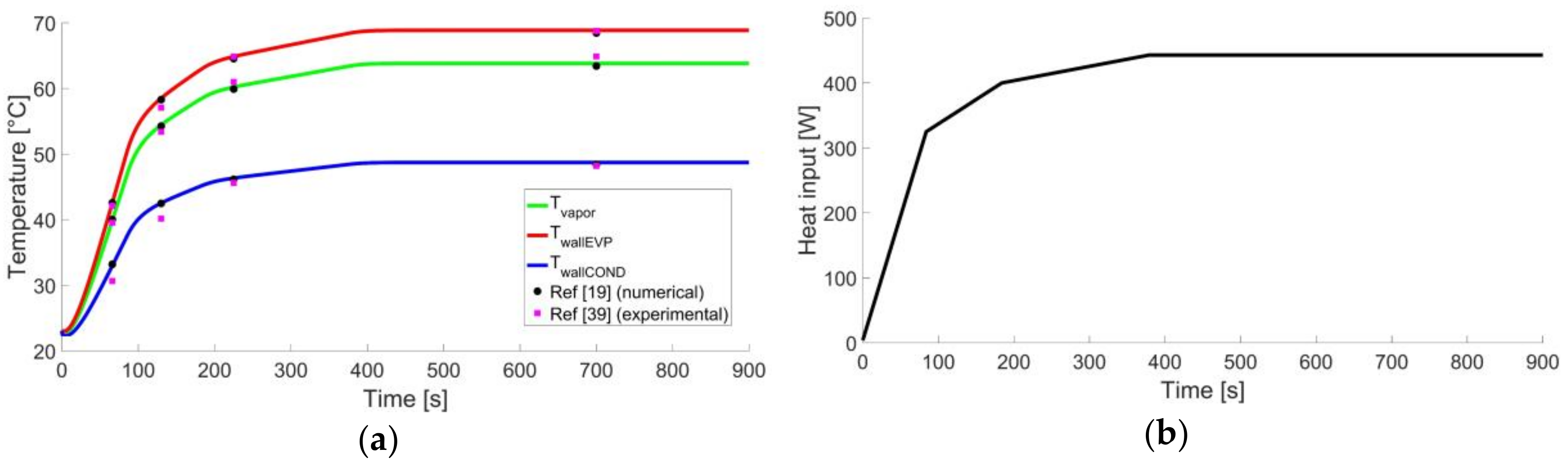
3.1. Transient Behaviour Validations

To validate the dynamic predictions of the presented model, the experimental results of Huang et al. [39] and the numerical results of Ferrandi et al. [19] for a cylindrical copper-water heat pipe with a copper screen-wick is used. The copper heat pipe has an outer diameter of 1.91 cm and an inner diameter of 1.73 cm. The length of the heat pipe is 89 cm, with a long evaporator section of 60 cm and shorter condenser section of 20 cm. A water jacket is used to achieve convective cooling at the condenser. All the other parameters used in the experiment or derived from the experiment (e.g., effective power throughput, convective heat transfer coefficient in the cooling jacket, etc.) are given in detail in [19].
The temperature evolution predictions of the presented model, its comparison with the experimental and numerical results of previous works and boundary condition at the evaporator are shown in Figure 2. For both the presented model and the experimental results from [39], displayed temperatures are the average of the sections. In this case, the modelled heat pipe is divided into only nine cells in the axial direction.
As seen in Figure 2, the presented model shows excellent agreement with the numerical results of [19] and the experimental results of [39]. The reason for the small difference of 2.0% between the current model and the experimental results is attributed to the measurement uncertainty as well as the derived parameters. Since these derived parameters are extracted from [19], the deviation between the results of [19] and the current model is limited to 0.5% only.

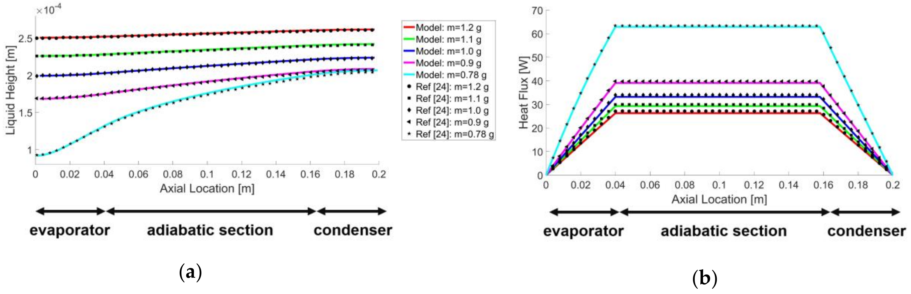
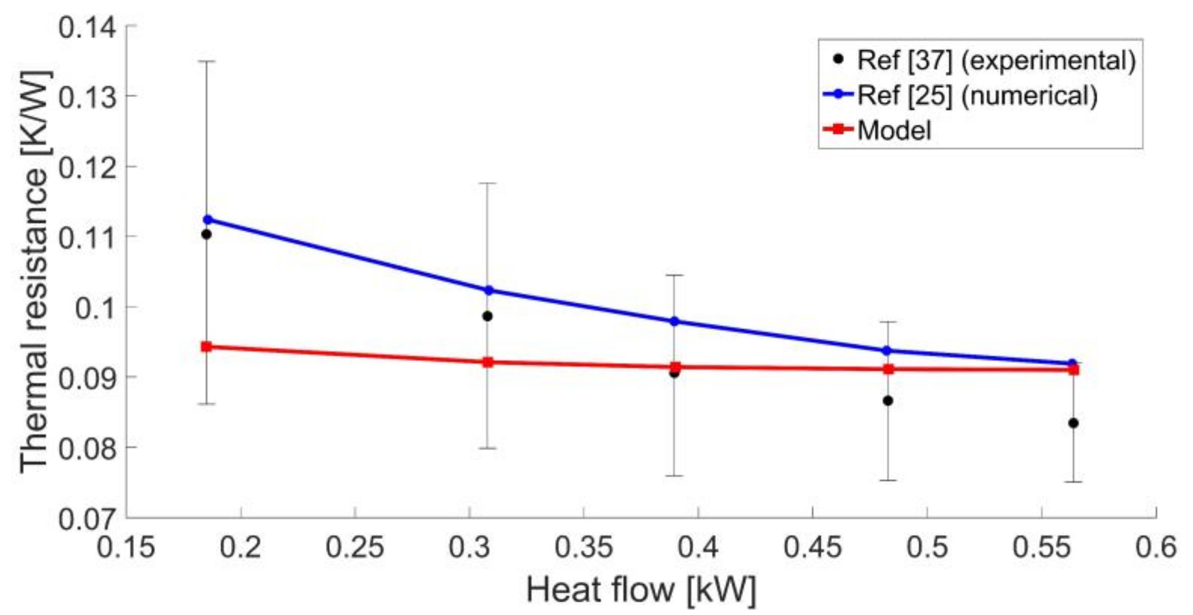
3.2. Steady-State Behaviour Validations

To validate the results of the current model at steady-state, first, the results of the analytical work by Bertossi et al. [24] for a rotating heat pipe are used. Following this validation, the results of the experimental work and the numerical work by Song et al. [25,37] are compared to the current model.
In [24], the simulated RHP has an inner diameter of 0.4 cm and a length of 20 cm. The model results are investigated for different fill ratios and heat inputs, keeping the rotational speed fixed at 3000 RPM and the temperature difference between the evaporator and adiabatic section wall temperatures at 10 °C. Since model parameters such as the fluid properties are explicitly documented in [24], differences between the model predictions would be caused by the underlying assumptions and model limitations (e.g., mesh size) only.
The results of the liquid height distribution and the heat flow along the heat pipe are compared in Figure 3. As stated in Section 2.5, a finer mesh in the axial direction is required for very low fill ratios. Therefore, the axial mesh number is 108 for the lowest fill ratio case and 36 for all other cases.
Again, the agreement between the presented model and the reference steady-state model [24] is excellent. The average deviation in the heat flow along the heat pipe between the two models is calculated as 2.1%. This deviation is attributed to the fact that the conduction in the liquid layer is approximated as a conduction through a plane layer in Bertossi et al [24]. In the presented model, thermal resistance through the liquid layer is calculated with the radial resistance as given in Equation (1). In the results, it is seen that a heat flow of 63 W is required to obtain 10 °C difference between the evaporator and the adiabatic section for the lowest fill ratio case, whereas this value is only 26 W for the highest fill ratio. This is caused by the higher thermal resistance of the liquid component when the liquid film is thicker as it is observed in Figure 3a.
Another validation is performed for a copper-water cylindrical RHP with an outer diameter of 25.4 mm and a total length of 400 mm [37]. The heat pipe is filled with 6.3 g of distilled water and the rotational speed is 4000 RPM. During the experiments, heat is applied with an inductor coil, whereas a water jacket is used for cooling. For both the experiments and the numerical model, overall thermal resistance of the heat pipe is plotted against varying heat input. During the validation, natural convection at the evaporator is accounted for [25].
The results of the current model, the experiments from [37] and the numerical model from [25] are shown in Figure 4. The uncertainties of the thermal resistances caused by measurement errors are computed for a 95% confidence interval.
It is seen that the agreement of the current model with the experimental results is good. All of the calculated thermal resistances are within the uncertainty limits of the experimental results. The predictions of the current model are also in line with the results of the numerical model by Song et al. [25], having an average deviation of 6.2%. Some of this deviation can be attributed to the fact that axial conduction through the copper wall is not accounted for in [25]. This results in estimating a higher overall thermal resistance compared to the prediction of the current model.

3.3. Computational Efficiency

In order to quantify the computational efficiency of the model, two cases presented in 3.2 are executed using different mesh sizes until they reached steady-state. The comparison between different mesh sizes is made in terms of computational time and relative error in the computed heat transferred through the heat pipe. The results are presented in Table 1, in reference to the execution with the finest mesh (80 cells in the axial direction).
It is observed that a doubling in the mesh size approximately triples the computational time. On the other hand, the relative error does not change significantly for the tested cases when the mesh size is halved. As noted in Section 2.5, the accuracy is compromised more when the fill ratio is lower. However, the relative error is kept at an acceptable level even with the lowest mesh size.

3.4. Parametric Study

The results of the presented model are explored in more detail at various boundary conditions for both SCHP and RHP.
A heat pipe with container material SAE 304 using water as a medium was examined. The heat pipe has a length of 0.2 m, inner diameter of 0.045 m and a wall thickness of 1 mm. In the case of the SCHP, the wick is also made of SAE 304 and it has a thickness of 1 mm. The wick porosity is 0.9, the wick permeability is 0.0015 mm2 and the effective pore radius is 54 μm, similar to the wick properties reported in [21]. The fill ratio is 4.4%. The lengths of the evaporator and the condenser are 0.05 m each. The heat input and output are fixed at 200 W.

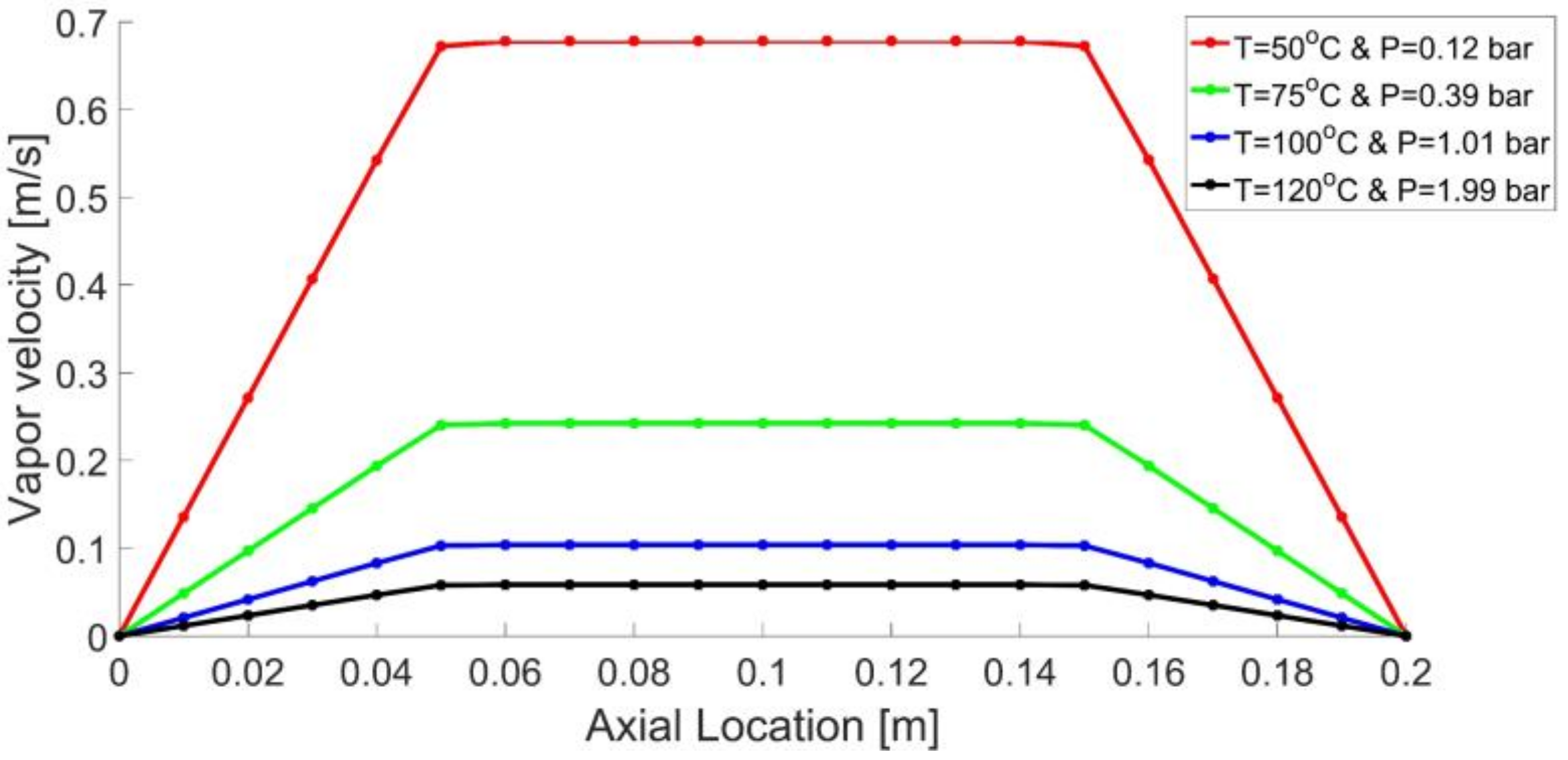
3.4.1. Effect of Operating Temperature on Vapor Dynamics

For a heat pipe operating at steady-state, the operating temperature and the heat flow have a direct influence on the vapor velocity. Using the presented model, the effect of the operating temperature on vapor dynamics is investigated for four cases. The operating temperatures for these four cases are 50 °C, 75 °C, 100 °C and 120 °C, respectively. For all cases, same amount of heat is transferred. The simulation results for the vapor velocity along the heat pipe are shown in Figure 5.
It is observed that the vapor velocity shows an increasing trend when the operating temperature becomes lower. The maximum vapor velocity was obtained with the vapor temperature of 50 °C where the vapor velocity was 0.7 m/s. This is caused by a low vapor density because of the low vapor pressure at low temperature. To be able to calculate the vapor velocity is especially important in order to avoid the sonic limit. At or near the sonic limit, the temperature distribution along the vapor channel becomes significantly non-isothermal. The results also show that the vapor velocity profile at the evaporator and the condenser is nearly linear, which together with the boundary conditions of a uniform heat flux at the evaporator and condenser implies that the evaporator and condenser temperatures are uniform.

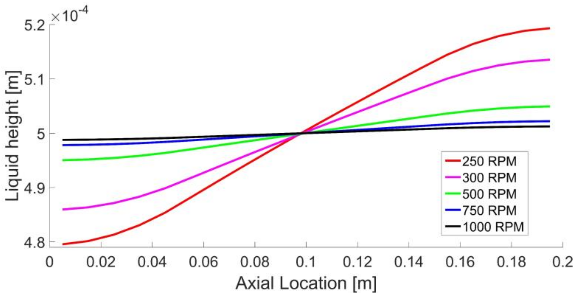
3.4.2. Effect of Rotational Speed on Liquid Height Distribution

The rotational acceleration, along with the liquid head, is the driving force of liquid transport from the condenser to the evaporator for a rotating heat pipe. An increase in the rotational speed allows for the same amount of liquid transported with a lower liquid head. Five cases with rotational speeds of 250, 300, 500, 750, and 1000 RPM are compared in Figure 6.
The comparison between the cases clearly shows that the head required to replace the same amount of liquid is much lower when the rotational speed is increased. With a rotational speed of 250 RPM, the required head is 40 μm, whereas it is only 2.5 μm for a rotational speed of 1000 RPM. Therefore, while determining the minimum fill ratio for a rotating heat pipe application, the effect of the centrifugal force on the liquid height distribution needs to be taken into account. For heat pipes operating at lower rotational speed, more liquid is needed to prevent dry-out.

4. Conclusions

In the presented work, a new engineering model applicable to both cylindrical SCHPs and RHPs is developed. The numerical model describes the transient behavior of the heat pipe with a 2D axisymmetric geometry.
The model offers sufficient accuracy and level of detail concerning the interior dynamics of the heat pipe in combination with fast execution. At each axial location, the heat pipe is divided into three components, namely the wall, the liquid and the vapor. The liquid and the vapor cells in each axial location are allowed to change size radially so that the total volume is conserved. This gives the unique advantage to track the liquid/vapor interface without the need for fine meshing or re-meshing. In order to achieve this, the equations for mass, momentum and energy are adapted to the meshing method.
The developed model shows excellent agreement with experimental, numerical and analytical studies found in the literature for SCHPs and RHPs. The model can be used to efficiently explore load cases, for example changing operating temperature and rotational speed.
With this model, the interior dynamics of cylindrical heat pipes can be simulated with a low computational cost and high accuracy. This is instrumental in engineering and design applications where the information that is supplied by thermal network models is not detailed enough, yet the computational cost of CFD cannot be afforded.

Author Contributions

Conceptualization, M.C., G.P. and W.d.J.; Methodology, M.C., G.P. and B.J.B; Software, M.C.; Validation, M.C.; Writing, M.C.; Review & Editing, G.P., D.v.E., W.d.J.; Supervision, G.P., D.v.E., W.d.J.; Project Administration, G.P., D.v.E., W.d.J. and B.J.B.

Funding

This research received no external funding.

Acknowledgments

This work is part of a collaboration project named “Heat Pipe Assisted Annealing” between Tata Steel, TU Delft and Drever International. The assistance of the collaborating project members is gratefully acknowledged.

Conflicts of Interest

The authors declare no conflict of interest.

Nomenclature

A Cross-sectional area of the node in the axial direction, m
C 1 C 6 Coefficients of polynomial velocity profile
c p Specific heat, J/(kg·K)
d Thickness, m
f Correction coefficient for capillary pressure
h Heat transfer coefficient, W/(m2·K)
H f g Latent heat, J/kg
K Wick permeability, m2
k Thermal conductivity, W/(m·K)
L Heat pipe total length, m
M Molecular weight, kg/mol
m Mass, kg
m ˙ Mass flow rate, kg/s
Q ˙ Heat flow, W
Q ˙ Heat flux, W/m2
p Pressure, Pa
R Thermal resistance, K/W
g Universal gas constant, J/(mol·K)
r Radial coordinate, radius, m
𝓇 Radii of the resistance, m
T Temperature, K
t Time, s
u Velocity, m/s
V Volume, m3
z Axial coordinate
Greek symbols
γ Viscous term in momentum equation, kg/(m2·s2)
Δ Difference
Δ z Length of the node in the axial direction, m
Δ z Distance between the adjacent node centers, m
ε Porosity
μ Viscosity, Pa·s
ρ Density, kg/m3
σ Surface tension, N/m
Φ Angular coordinate
ω Rotational speed, rad/s
Subscripts
c Capillary
c o n v Convection
e f f Effective
i Inner
Liquid
o Outer
p h Phase change
r a d Radiation
s Solid
v Vapor
w Wick
Ambient

References

  1. Faghri, A. Review and advances in heat pipe science and technology. J. Heat Trans. 2012, 134, 123001. [Google Scholar] [CrossRef]
  2. Reay, D.; McGlen, R.; Kew, P. Heat pipes: Theory, design and applications, 6th ed.; Butterworth-Heinemann: Oxford, UK, 2014; pp. 15–43. ISBN 978-0-08-098266-3. [Google Scholar]
  3. Zuo, Z.J.; Faghri, A. A network thermodynamic analysis of the heat pipe. Int. J. Heat Mass Transf. 1998, 41, 1473–1484. [Google Scholar] [CrossRef]
  4. Grover, G.M.; Cotter, T.P.; Erickson, G.F. Structures of very high thermal conductance. J. Appl. Phys. 1964, 35, 1990–1991. [Google Scholar] [CrossRef]
  5. Ballback, L.J. The operation of a rotating wickless heat pipe. Ph.D. Thesis, US Naval Postgraduate School, Monterey, CA, USA, 1969. [Google Scholar]
  6. Kim, K.S.; Won, M.H.; Kim, J.W.; Back, B.J. Heat pipe cooling technology for desktop PC CPU. Appl. Therm. Eng. 2003, 23, 1137–1144. [Google Scholar] [CrossRef]
  7. Lin, L.; Ponnappan, R.; Leland, J. High performance miniature heat pipe. Int. J. Heat Mass Transf. 2002, 45, 3131–3142. [Google Scholar] [CrossRef]
  8. Ivanova, M.; Avenas, Y.; Schaeffer, C.; Dezord, J.B.; Schulz-Harder, J. Heat pipe integrated in direct bonded copper (DBC) technology for cooling of power electronics packaging. IEEE Trans. Power Electron. 2006, 21, 1541–1547. [Google Scholar] [CrossRef]
  9. Vasiliev, L.L. Micro and miniature heat pipes—Electronic component coolers. Appl. Therm. Eng. 2008, 28, 266–273. [Google Scholar] [CrossRef]
  10. Turner, R. The “constant temperature” heat pipe—A unique device for the thermal control of spacecraft components. In Proceedings of the AIAA 4th Thermophysics Conference, San Francisco, CA, USA, 16–18 June 1969; pp. 69–632. [Google Scholar] [CrossRef]
  11. Liang, J.; Gan, Y.; Li, Y. Investigation on the thermal performance of a battery thermal management system using heat pipe under different ambient temperatures. Energy Convers. Manag. 2018, 155, 1–9. [Google Scholar] [CrossRef]
  12. Kuboth, S.; König-Haagen, A.; Brüggemann, D. Numerical Analysis of Shell-and-Tube Type Latent Thermal Energy Storage Performance with Different Arrangements of Circular Fins. Energies 2017, 10, 274. [Google Scholar] [CrossRef]
  13. Jen, T.C.; Gutierrez, G.; Eapen, S.; Barber, G.; Zhao, H.; Szuba, P.S.; Labataille, J.; Manjunathaiah, J. Investigation of heat pipe cooling in drilling applications.: Part I: Preliminary numerical analysis and verification. Int. J. Mach. Tool Manu. 2002, 42, 643–652. [Google Scholar] [CrossRef]
  14. Ponnappan, R.; He, Q.; Leland, J. Test results of a high-speed rotating heat pipe. In Proceedings of the AIAA 32nd Thermophysics Conference, Atlanta, GA, USA, 23–25 June 1997; p. 2543. [Google Scholar] [CrossRef]
  15. Kukharskii, M.P. Closed evaporative cooling of rotating electrical machines. J. Eng. Phys. 1974, 27, 1090–1096. [Google Scholar] [CrossRef]
  16. Groll, M.; Krahling, H.; Munzel, W.D. Heat pipes for cooling of an electric motor. J. Energy 1978, 2, 363–367. [Google Scholar] [CrossRef]
  17. Celik, M.; Devendran, K.; Paulussen, G.; Pronk, P.; Frinking, F.; de Jong, W.; Boersma, B.J. Experimental and numerical investigation of contact heat transfer between a rotating heat pipe and a steel strip. Int. J. Heat Mass Transf. 2018, 122, 529–538. [Google Scholar] [CrossRef]
  18. Xuan, Y.; Hong, Y.; Li, Q. Investigation on transient behaviors of flat plate heat pipes. Exp. Therm. Fluid Sci. 2004, 28, 249–255. [Google Scholar] [CrossRef]
  19. Ferrandi, C.; Iorizzo, F.; Mameli, M.; Zinna, S.; Mameli, M. Lumped parameter model of sintered heat pipe: Transient numerical analysis and validation. Appl. Therm. Eng. 2013, 50, 1280–1290. [Google Scholar] [CrossRef]
  20. Wits, W.W.; Kok, J.B. Modeling and validating the transient behavior of flat miniature heat pipes manufactured in multilayer printed circuit board technology. J. Heat Trans. 2011, 133, 081401. [Google Scholar] [CrossRef]
  21. Tournier, J.M.; El-Genk, M.S. A heat pipe transient analysis model. Int. J. Heat Mass Transf. 1994, 37, 753–762. [Google Scholar] [CrossRef]
  22. Solomon, A.B.; Ramachandran, K.; Asirvatham, L.G.; Pillai, B.C. Numerical analysis of a screen mesh wick heat pipe with Cu/water nanofluid. Int. J. Heat Mass Transf. 2014, 75, 523–533. [Google Scholar] [CrossRef]
  23. Daniels, T.C.; Al-Jumaily, F.K. Investigations of the factors affecting the performance of a rotating heat pipe. Int. J. Heat Mass Transf. 1975, 18, 961–973. [Google Scholar] [CrossRef]
  24. Bertossi, R.; Guilhem, N.; Ayel, V.; Romestant, C.; Bertin, Y. Modeling of heat and mass transfer in the liquid film of rotating heat pipes. Int. J. Therm. Sci. 2012, 52, 40–49. [Google Scholar] [CrossRef]
  25. Song, F.; Ewing, D.; Ching, C.Y. Fluid flow and heat transfer model for high-speed rotating heat pipes. Int. J. Heat Mass Transf. 2003, 46, 4393–4401. [Google Scholar] [CrossRef]
  26. Uddin, Z.; Harmand, S.; Ahmed, S. Computational modeling of heat transfer in rotating heat pipes using nanofluids: A numerical study using PSO. Int. J. Therm. Sci. 2017, 112, 44–54. [Google Scholar] [CrossRef]
  27. Hassan, H.; Harmand, S. Effect of using nanofluids on the performance of rotating heat pipe. Appl. Math. Model. 2015, 39, 4445–4462. [Google Scholar] [CrossRef]
  28. Harley, C.; Faghri, A. Two-dimensional rotating heat pipe analysis. J. Heat Trans. 1995, 117, 202–208. [Google Scholar] [CrossRef]
  29. Baker, J.; Ponnappan, R.; Leland, J. A computational model of transport within a rotating heat pipe—Part 1—Formulation. In Proceedings of the AIAA 37th Aerospace Sciences Meeting and Exhibit, Reno, NV, USA, 11–14 January 1999. [Google Scholar] [CrossRef]
  30. Lian, W.; Chang, W.; Xuan, Y. Numerical investigation on flow and thermal features of a rotating heat pipe. Appl. Therm. Eng. 2016, 101, 92–100. [Google Scholar] [CrossRef]
  31. Zhu, N.; Vafai, K. Analysis of cylindrical heat pipes incorporating the effects of liquid–vapor coupling and non-Darcian transport—A closed form solution. Int. J. Heat Mass Transf. 1999, 42, 3405–3418. [Google Scholar] [CrossRef]
  32. Aghvami, M.; Faghri, A. Analysis of flat heat pipes with various heating and cooling configurations. Appl. Therm. Eng. 2011, 31, 2645–2655. [Google Scholar] [CrossRef]
  33. Hansen, G.; Næss, E.; Kristjansson, K. Analysis of a vertical flat heat pipe using potassium working fluid and a wick of compressed nickel foam. Energies 2016, 9, 170. [Google Scholar] [CrossRef]
  34. Nemec, P.; Čaja, A.; Malcho, M. Mathematical model for heat transfer limitations of heat pipe. Math. Comput. Model. 2013, 57, 126–136. [Google Scholar] [CrossRef]
  35. Chan, S.H.; Kanai, Z.; Yang, W.T. Theory of a rotating heat pipe. J. Nucl. Energy 1971, 25, 479–487. [Google Scholar] [CrossRef]
  36. Lin, L.; Faghri, A. Heat transfer in micro region of a rotating miniature heat pipe. Int. J. Heat Mass Transf. 1999, 42, 1363–1369. [Google Scholar] [CrossRef]
  37. Song, F.; Ewing, D.; Ching, C.Y. Heat transfer in the evaporator section of moderate-speed rotating heat pipes. Int. J. Heat Mass Transf. 2008, 51, 1542–1550. [Google Scholar] [CrossRef]
  38. Song, F.; Ewing, D.; Ching, C.Y. Experimental investigation on the heat transfer characteristics of axial rotating heat pipes. Int. J. Heat Mass Transf. 2004, 47, 4721–4731. [Google Scholar] [CrossRef]
  39. Huang, L.; El-Genk, M.S.; Tournier, J.M. Transient performance of an inclined water heat pipe with a screen wick. In Proceedings of the ASME 29th National Heat Transfer Conference, Atlanta, GA, USA, 8–11 August 1993. [Google Scholar]
Figure 1. Model geometry and cells.
Energies 11 03458 g001
Figure 2. Transient modelling results: (a) Comparison with Ferrandi et al. [19] and Huang et al. [39]; (b) Heat input at the evaporator.
Energies 11 03458 g002
Figure 3. Steady-state modelling results and comparison with Bertossi et al. [24]: (a) Liquid height distribution; (b) Heat flow along the heat pipe.
Energies 11 03458 g003
Figure 4. Overall thermal resistance results and comparison with the experiments by Song et al. [37] and the numerical model by Song et al. [25].
Energies 11 03458 g004
Figure 5. Vapor velocity along the heat pipe at different operating temperatures.
Energies 11 03458 g005
Figure 6. Liquid height distribution along the heat pipe.
Energies 11 03458 g006
Table 1. Computational efficiency.
CaseMesh SizeComputational TimeRelative Error
m = 1.2 g80100% (Ref)0% (Ref)
4028.7% <0.01%
209.0%0.01%
103.2%0.06%
m = 0.9 g80100% (Ref)0% (Ref)
4029.4%0.04%
209.6%0.16%
103.4%0.55%

