Article

Deep Highway Networks and Tree-Based Ensemble for Predicting Short-Term Building Energy Consumption

1
BRE Trust Centre for Sustainable Engineering, School of Engineering, Cardiff University, Cardiff CF24 3AA, UK
2
Commissariat á l’énergie atomique et aux énergies alternatives (CEA), CEA Tech en Région (CTREG), Département Grand Ouest (DGDO), 44340 Bouguenais, France
*
Author to whom correspondence should be addressed.
Energies 2018, 11(12), 3408; https://doi.org/10.3390/en11123408
Submission received: 1 October 2018 / Revised: 19 November 2018 / Accepted: 27 November 2018 / Published: 5 December 2018

Abstract

:
Predictive analytics play a significant role in ensuring optimal and secure operation of power systems, reducing energy consumption, detecting fault and diagnosis, and improving grid resilience. However, due to system nonlinearities, delay, and complexity of the problem because of many influencing factors (e.g., climate, occupants’ behaviour, occupancy pattern, building type), it is a challenging task to get accurate energy consumption prediction. This paper investigates the accuracy and generalisation capabilities of deep highway networks (DHN) and extremely randomized trees (ET) for predicting hourly heating, ventilation and air conditioning (HVAC) energy consumption of a hotel building. Their performance was compared with support vector regression (SVR), a most widely used supervised machine learning algorithm. Results showed that both ET and DHN models marginally outperform the SVR algorithm. The paper also details the impact of increasing the deep highway network’s complexity on its performance. The paper concludes that all developed models are equally applicable for predicting hourly HVAC energy consumption. Possible reasons for the minimum impact of DHN complexity and future research work are also highlighted in the paper.

1. Introduction

Globally, there are growing concerns regarding the total energy consumption from the building sector, which is one of the main substantial users of energy. Buildings account for 40% of the world’s total energy consumption and contribute towards 30% of the total CO2 emissions [1]. According to the current European Union (EU) roadmap, the EU is committed to reducing greenhouse gas emission by 20%, reaching a share of renewable energy in gross final energy by 20%, and reducing total primary energy consumption by 20%—by 2020 as compared to the 1990 levels [2]. In the non-domestic sector, hotels and restaurants are the third largest consumers of energy, accounting for 30%, 18%, 16% and 14% in Spain, France, the UK and the USA, respectively [3,4]. In Greece and Spain, hotels are responsible for about 1/3 of the total energy demand [5]. In hotels, nearly half of the electricity is used for space conditioning purposes [6]. Because of a significant amount of energy consumption, there have been increasing concerns on hotels’ energy use and efforts to effectively manage energy consumption. Predicting energy consumption over a wide range of time horizons is one of the key features of smart girds. It allows for building managers/owners to make informed decisions; e.g., increasing share of renewable energy sources and shifting energy use to off-peak times.

1.1. Context and Objectives

The gap between actual measured performance and predicted energy performance of buildings, typically addressed as ’the performance gap’, is an increasing concern for the building industry [7]. The gap can be explained by a wide range of factors that get amplified during the lifecycle of the building [8,9,10]. The energy performance gap negatively impacts occupants’ comfort and energy consumption. Therefore, it is critical for energy managers/building owners to identify causes of operational energy performance gap and to take countermeasures as quickly as possible. Different researchers have tackled this problem by identifying performance gap and fault detection and diagnosis using time-dependent and steady-state analytical modelling, data-driven modelling or knowledge-based methods. The objective of this paper is to detail the performance of the developed machine learning models, which could be used to identify an energy performance gap, make informed decisions by energy managers/building owners, and detect and diagnose faults in a hotel building.
Accurate prediction of energy consumption is an exigent task due to system nonlinearities, delays, and complexity of the studied problem. Recently, a number of different techniques has been developed and applied to predict energy consumption at a building level. These techniques can be divided into data-driven and first principle methods.
First principle-based methods (e.g., TRNSYS, EnergyPlus, DOE-2) require detailed information about building features, and installed energy systems. These methods, because of their multi-domain modelling capabilities, often enable users to assess different design strategies with lower uncertainties [11]. However, because of the complex nature of human behaviour inside buildings, these methods do not perform well for occupied buildings [12]. Physical models can be computationally intensive and therefore an exhaustive exploration of parameter space for optimal control strategies could be infeasible. Because of these factors, a physical model of a building/energy system is mostly avoided, and a simpler, efficient and accurate data driven model is created. Data-driven techniques do not require detailed information about building characteristics or heating, ventilation and air conditioning (HVAC) systems. However, the computational cost of learning and hyper-parameters could be high for data-driven models. The prediction accuracy is also influenced by the quantity and quality of the available training dataset. The authors acknowledge the fact that, for both data-driven and detailed models, there is a trade-off between computational cost and prediction accuracy. Mostly, data-driven techniques are better suited for near real-time optimisation applications as they need significantly less prediction time and require less prior information about the buildings of interest.
Accurate energy prediction models are used by facility managers and utilities to effectively schedule and control continuously fluctuating energy supply and demand, and avoid penalties that could occur due to the difference between predicted and consumed energy. Machine learning models are often the preferred choice for real-time control applications because of their fast response time as compared to detailed simulation models [3]. Due to instability issues, most of the widely used machine leaning techniques are likely to be unreliable. As the developed models in this paper could be used for optimal control, the stability of developed models is critical. In recent years, more advanced prediction methods (ensemble and deep learning) were developed to overcome the limitations of traditional methods.

1.2. Related Work

Deep-learning methods are one of the most efficient methods for classification problems and have been tested for numerous applications [13,14,15,16]. Among these methods, the recurrent neural network is capable of instantiating almost arbitrary dynamics and allowing the information flow to be “memorized” during the computation to enrich further processing. Recently, the performance of “Long Short-Term Memory” (LSTM)—a type of recurrent neural network method—has been tested in different research studies [17,18]. However, these techniques have been extensively applied in the vision domain; various other research works have also applied deep-learning methods for other research areas, e.g., cancer (diagnosis and detection) [19], chatbots and NLP (Natural Language Processing) [20], games (scoring and human-level playing) [21], and heart diseases [22]. One of the limitations of deep-learning methods was that their performance did not improve with the increase in network’s depth. Recently, a number of improvements have been performed to tackle this issue, e.g., by using recurrent like behaviour in feed-forward models (ResNets [23], Inception/Xception [24], Highways [25]), introducing reinforcement learning, previous input auto-encoding and incremental layer learning, and evolution of learning rules (e.g., dropout, Adam, Nesterov, batches, blurring inputs). These improvements have significantly enhanced the performance of deep-learning methods.
With the growth in performance of deep learning methods and despite the fact that historical prediction models are less complex, numerous studies in the past few months proposed diverse deep learning approaches for estimating building energy consumption [26] and forecast/prediction [27,28,29] with both feed-forward and recurrent neural network models. Optimization of energy consumption through reinforcement learning has also recently been studied with deep learning models [30]. Deep learning is being used either as a predictive modeling tool or a feature extractor as in [31]. The study also showed that the feature extraction property is of more interest than the predictive property itself, which does not perform better than eXtreme Gradient Boosting in this case. In most cases, deep learning models’ hyperparameters are empirically chosen and in only a few cases do these parameters span a large part of the possible space. In particular, studies often show comparison with simplest networks’ models.
Support vector machines (SVMs) are used in different applications of the building energy sector, e.g., Liang and Du [32] applied the SVM method for fault detection and diagnoses (FDD) by combining SVM, and model-based FDD. Mohandes et al. [33] predicted wind speed and Esen et al. [34] modeled a ground-coupled heat pump system by using SVM. Support vector machines have recently attracted researchers’ focus in the field of building energy prediction. To the authors’ knowledge, the first work was reported by Dong et al. [35]. The authors applied SVM to predict monthly building energy consumption in a tropical region (Singapore). Outside dry-bulb temperature, solar radiation, and relative humidity were considered as input parameters. The weather data were collected from a weather station which was approximately 12 miles away from the buildings under investigation. Although the percent error was small, the inaccuracies in the results due to weather data were not discussed in the paper. Li et al. [36] and Li et al. [37] predicted hourly cooling load in an office building in China. The author also compared SVM with different artificial neural networks. The SVM method performed slightly better than neural network methods. This was because of the structural risk minimization principle of SVM, which is used to minimize the upper bound of the generalization error. On the other hand, artificial neural networks minimized the training error. The performance of SVM can be enhanced through combination with other computational intelligence techniques. To enhance the SVM by reducing the effect of noise and outliers in the data set, Li et al. [38] proposed fuzzy SVM. As in load prediction, the old data are less important as compared to the new data. SVM does not have the ability to distinguish a new pattern and therefore the authors proposed the fuzzy SVM method.
Decision trees (DT) are used to classify a dataset into various predefined target values or classes. A DT based model can be represented by logical statements/rules. Decision tree, tree-based ensemble algorithms, in particular, are less popular in building energy research domains. Decision tree based methods were used by Yu et al. [39] to predict energy consumption. The authors concluded that decision tree based algorithms could be used to develop reliable models. A decision support model to reduce a school building’s electricity was developed by Hong et al. [40]. The authors used decision trees to form a group of educational buildings based on electricity consumption. Hong et al. [41] used decision trees for clustering a type of multifamily housing complex based on gas consumption. Tso and Yau [42] compared regression analysis, DT and artificial neural networks (ANN) for predicting electricity consumption. The authors concluded that the DT algorithm could be a viable option for predicting energy consumption. In a recent study by Ahmad et al. [3], the authors compared the performance of ANN and random forest (RF)—a tree-based ensemble algorithm. However, ANN performed marginally better in this study, and the authors concluded that both developed models have similar prediction accuracy and are equally applicable for predicting building energy consumption.
The paper compares the performance in prediction of hourly HVAC energy consumption of a hotel building by using three different machine learning (ML) approaches: deep highway networks, extremely randomised trees, and support vector regression. The research presented in this paper mainly addresses the following aspects:
  • The use of tree-based ensemble techniques and deep highway networks for predicting HVAC energy consumption from contextual data;
  • Studying the impact of networks’ depth on prediction performance of DHN models;
  • Demonstrate a prediction error of nearly 6% (normalised root mean square error)on hourly data for two of the best currently known machine learning algorithms (tree-based ensembles and deep learning).
The paper addresses the problem of predicting energy consumption of a hotel building. Predicting energy consumption of hotels and restaurants is a challenging task as it does not exhibit clear patterns. From the literature review, it was found that none of the previous studies compared the performance of recently developed deep learning and tree-based ensemble methods. The presented research work also discusses whether there is a need to develop deep learning models for high-resolution prediction of energy consumption or the current state-of-the-art methods are equally comparable.
The rest of the paper is organised as follows: the methodology of the developed models is presented in Section 2. In Section 2.1, principles of deep highway networks, support vector regression, and extremely randomised trees are described. Prediction results are described in Section 3, whereas Section 4 presents comparison between three developed machine learning models along with discussions. Concluding remarks are drawn at the end of the paper.

2. Materials and Methods

This section introduces the three proposed data-driven techniques for predicting HVAC energy consumption. The section also details training and testing datasets along with the evaluation metrics used for comparing the studied techniques. In this paper, SVR is used for comparison purposes, as it is one of the most widely machine learning techniques in a built environment research domain. Figure 1 illustrates the schematic overview of the proposed research. Historical weather, energy consumption and occupancy data were retrieved from a database for developing prediction models. The data was pre-processed for model development by removing outliers and treating missing values. The data was also normalised for SVR algorithms. Important features were selected by using random forest and extra trees algorithms. The models’ hyper-parameters were tuned by using either a genetic algorithm (GA) (for deep highway network) or a step-wise search method (support vector regression and extra trees).

2.1. Machine Learning Algorithms

Three data-driven algorithms for predicting energy consumption are introduced in this section. These algorithms include deep highway networks (DHN), extremely randomised trees (ET) and support vector regression (SVR).

2.1.1. Support Vector Regression

Support vector machines are one of the most widely used machine learning approaches to predict energy consumption. They are divided into two main categories: support vector classification (SVC) and support vector regression (SVR) [43]. As the name suggests, SVR is used for regression problems and the main objective is to find a relationship between input and output features while assuming that the joint distribution of the features is unknown. The SVR algorithms map the input data into a high-dimensional feature space through a nonlinear mapping and performing a linear regression in this feature space [43].
For modelling a process, suppose that the normalized inputs vector is X i (represents vector of input parameters) and Y i represents the outputs; then, the set of samples is defined as X i , Y i i = 1 N , where N is the length of training data set. The algorithm approximates the relationship between the outputs and inputs, while projecting input space in a higher dimensional space. In the present work, we make use of the framework defined in [44,45]:
Y = f X = W · ϕ X + b ,
where ϕ X represents the high-dimensional space, which is nonlinearly mapped from the input data. The coefficients W and b are estimated by using Equation (2) i.e., by minimising a regularised risk function [44,45].
M i n i m i z e : 1 2 W 2 + C 1 N N i = 1 L ε Y i , f X i ,
L ε Y i , f X i = 0 , i f Y i f X i ε , Y i f X i ε , o t h e r s .
Minimizing W 2 ensures as small W as possible. In the above equations, C is a penalty parameter (also known as regularisation parameter) that determines the balance between model flatness and tolerance with regard to errors that are larger than ε . The empirical error is denoted by the second term of Equation (2), which is measured by the ε -intensity loss function (Equation (3)). The loss is zero, if the predicted value is within the ε -tube. On the other hand, the loss is the difference between the radius ε of the tube and predicted error, if the predicted value is outside the tube [36]. In order to relax constraints in the estimation of W and b, slack variables ζ 1 and ζ 1 are introduced leading the above equation to become the primal objective function given by Equation (4) [44,45]:
M i n i m i z e ζ 1 , ζ 1 , W , b : 1 2 W 2 + C 1 N N i = 1 ( ζ 1 + ζ 1 ) ,
S u b j e c t t o : Y i W · ϕ x i b ε + ζ 1 , W · ϕ x i + b ε + ζ 1 , i = 1 , 2 , , N , ζ 1 0 ζ 1 0 .
This primal form of the optimization problem can be solved expressing the Lagrangian and then the dual form of the optimization problem [44,45].
Finally, the Mercer kernel K is defined as:
K X i , X j = e x p X i X j 2 δ 2 ,
which allows for expressing the inner products in the infinite dimensional features space ϕ so that Equation (1) becomes [44,45]:
Y = f X = N i = 1 α i α i K X i , X + b ,
where α i , α i are the Lagrange multipliers (constrained to be 0 ) and N the number of support vectors.
The normalized predicted output Y, which is obtained from an SVR model, should be transformed into the actual prediction value by using the following equation:
q ^ = q m i n + Y · q m a x q m i n .

2.1.2. Deep Highway Networks

Deep highway network (DHN) is a concept introduced in [25] by taking advantage of some of the properties of LSTM models in a purely feedforward fashion. In this work, the model proposed proved to be more stable in learning with an increase in the number of hidden layers than previous fully connected feedforward deep neural network models. This ability is obtained by introducing the following concepts. Generally, a feedforward Neural Network transformation of the input is given in Equation (8) [29]:
y = H ( x , W H ) .
In the above equation, y is the output of the network, and H is the nonlinear transformation applied to the input x and weighted by a parameters matrix W H . H can consist of multiple layers of nonlinear transformation and their corresponding weights. Each of these layers receives inputs from the preceding layer’s outputs and outputs to the next layer. In a simplified form, a highway network can be defined by Equation (9) [29]:
y = H ( x , W H ) · T ( x , W T ) + x · C ( x , W C ) .
The transform gate, T ( x , W T ) , transforms the input, whereas the carry gate ( x , W C ) allows for carrying input in a possibly unchanged form through different layers of the network, depending on the weights applied. This property resembles the residual behavior of ResNets, where unchanged input is propagated in the deep structure of the network, helping the network to keep learning even with a high number of hidden layers (efficient ResNets can have up to 1000 layers in recent works [46]). Similarly to the work of Srivastava et al. [25], we used a carry gate defined by C = 1 T . The resulting transformations achieved by the network are summarized in Equation (10) [29]:
y = H ( x , W H ) · T ( x , W T ) + x · ( 1 T ( x , W T ) ) .
Rectifier Linear Units (ReLu) [47] are used to populate the regular hidden layers and transform gate layers use a sigmoidal activation function. ReLu units are defined by Equation (11) [29]:
y = m a x ( 0 , x ) ,
with
x = K i = 1 w i x i .
In the above equation, w i x i is the weighted output value of the connected input neurons.

2.1.3. Extremely Randomized Trees

Extremely randomized trees or Extra-Trees (ET) [48] introduce stochasticity during the induction production of classical decision trees [49]. ET was developed as an extension of another tree-based ensemble method (random forest) to be a more computationally efficient algorithm. From several experiments, it was found that Extra-Trees (ET) outperform other tree-based methods, including random forests (RF) [50]. The key difference between RF and ET are highlighted in [51]: (1) ET uses the entire data set for training a model (i.e., it does use tree bagging), whereas a random forest algorithm uses a bootstrap replica for training a machine learning model, and (2) ET randomly picks the best feature along with the corresponding value to split the node. Due to these main differences, ET is less likely to overfit a dataset and has reported better performance [48]. The ET splitting procedure for numerical attributes is detailed in [48]. ET relies on three main hyper-parameters that will be further optimized as detailed in Section 3.3. It consists of three factors: K is the number of randomly selected variables for splitting a node, n m i n represents the minimum number of samples required for splitting an internal node, and M, the number of trees formed in the ensemble model [45].

2.2. Data Description

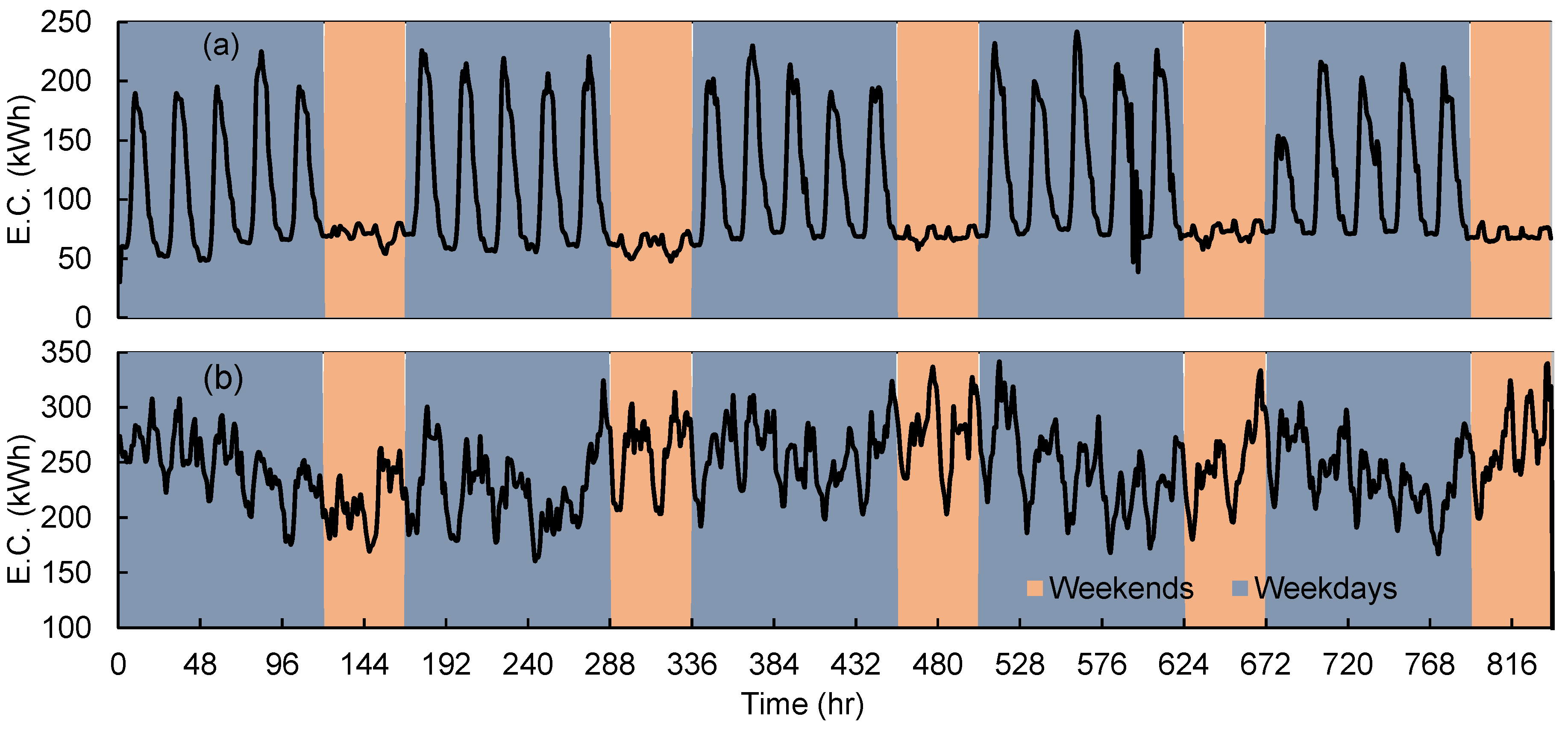
The historical dataset of HVAC energy consumption was gathered from a hotel building in Madrid, Spain. Social parameters (e.g., number of rooms booked, the total number of guests on a particular day) were also retrieved from the hotel’s reservation system. Weather parameters were also collected from a nearby weather station.As hotels and restaurants do not exhibit clear energy consumption patterns as compared to other building types e.g., school buildings, which makes prediction a challenging task. Figure 2 shows electricity consumption of a school in Wales, UK and a hotel building in Madrid, Spain. It can be seen that there is a clear energy consumption pattern for the school building as the energy consumption is lower during the night and weekends. On the other hand, this is not the case for the hotel building.
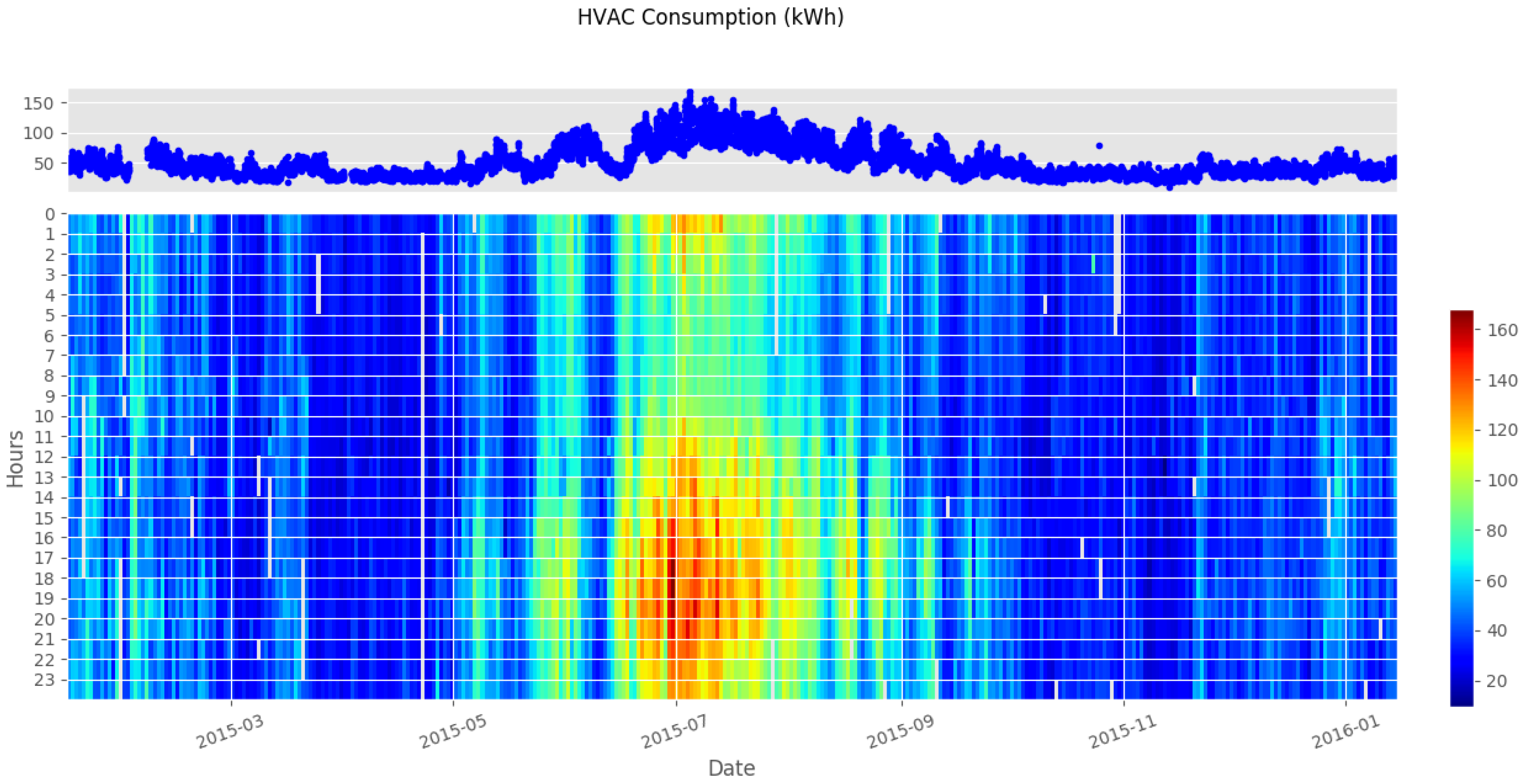
For this study, one and a half year data was collected from the hotel’s building management system (BMS) with a collection interval of 5 min. The collected dataset contained air temperature, relative humidity, wind speed, dew point air temperature, hour of the day, day of the week, month of the year, total rooms booked, total number of guests and value of HVAC energy consumption. Table 1 summarizes the variables used in the development of prediction models. Figure 3 shows the hourly HVAC consumption values of the studied building from 15 January 2015 to 15 January 2016. Training data is taken as 80% of the dataset such that the first 7680 samples were used in training and validation phases and the remaining 3290 samples composed the test dataset. For each algorithm training, the dataset was shuffled with identical random seeds to ensure that the exact same training set was used.

2.3. Model Evaluation Metrics

To evaluate the predictive performance of the developed models, four different metrics, i.e., root mean squared error (RMSE), mean absolute error (MAE), coefficient of determination (R2) and normalised root mean squared error (NRMSE) were used. Determination coefficient is used to measure the correlation between the actual and predicted HVAC energy consumption values. The remaining three metrics are described as below:
R M S E = i = 1 N ( y i y ^ i ) 2 N
M A E = 1 N i = 1 N | y ^ i y i |
N R M S E = R M S E y m a x y m i n
where y ^ i is the predicted value, y i is the actual value, N is the total number of samples, and y max and y min are the maximum and minimum values of actual HVAC energy consumption, respectively.
For this work, the implementation of extra trees and support vector regression included in the scikit-learn (a machine learning library for Python programming language) [52]. DHN was implemented in Python programming language. All developed models are encapsulated in a Python library to allow online data acquisition and predictions updates. It is worth mentioning that the model presented by Dieleman [53] was adapted for this paper. The models were trained and tested on personal computers (Intel Core i7 3.20 GHz with 32 GB of installed memory (for SVR and ET) and Intel Xeon 32 CPU 1.30 GHz with 64 GB of installed memory (for DHN models)).

3. Results

This section details the impact of different algorithms associated with hyper-parameters on a model’s performance. A stepwise searching method was used to find optimal hyper-parameters values for SVR and ET models. For deep highway network models, a genetic algorithm based method was used for hyper-parameter tuning.

3.1. DHN Hyper-Parametric Tuning

A two stage hyper-parameter estimation was performed to find the best parameters for deep highway network models. At the first stage, a grid search was performed to highlight the best range of hyper-parameters. DHN models were trained by using a 5-fold cross-validation process, and setting a batch size inside epochs to 64 samples. Mean squared error was used as a criterion to evaluate training process. A Nesterov accelerated SGD (Stochastic Gradient Descent) update [54] was applied during the training phase. During the second stage, hyper-parameters of DHN were optimized using a genetic algorithm. The optimization problem and objective function of DHN hyper-parametric tuning can be represented by Equation (16):
min x ϵ X f ( x )
where: x is the decision variables vector [ x 1 , x 2 , , x n ] , n being the number of decision variables; and f ( x ) is the objective function. In this case, eight decision variables were used i.e., number of neurons in each hidden layer, number of hidden layers, number of training epochs, learning rate, momentum, output layer activation function, bias value of gate layers neurons, and model inputs. Among the input variables of the dataset, preliminary studies showed that the most impacting variables were: outside temperature, relative humidity, number of guests and HVAC consumption values. The model inputs’ decision variable states how many preceding values of each of these four input variables are used as input to the DHN model. Equation (16) is subject to ranges of values for each decision variable listed in Table 2.
The objective function of the problem is to minimize the normalized root mean squared error (NRMSE) on a testing dataset. The genetic algorithm optimisation was performed by considering 300 generations with a population size, mutation rate and crossover rate of 30, 0.1 and 0.5, respectively. The tournament selection method was used for selecting the five best individuals from a population. It is also worth mentioning that various previous values for input variables were also tried to improve the predictive performance of a DHN model.
Table 3 shows the 10 best performances of DHN models in terms of NRMSE. For each model, different performance metrics are applied. The results showed that, for the top 10 best models, the prediction accuracy was always greater than R2 value of 0.84. It was found that several combinations of networks can achieve best performance, and generally no hyper-parameter drives the predictive performance of the models. Experimental results showed that best performance was obtained with an input dimension of 73 i.e., taking as input the previous 24 h of outdoor dry-bulb air temperature, air relative humidity and HVAC energy consumption and only the past value of the number of guests. However, it is worth mentioning that the increase in performance is small as compared to the increase in the complexity of the model. Results depict that a higher number of layers does marginally improve the performance; however, the best five performances were obtained by using one-layered networks. In order to further investigate the influence of model complexity, Table 4 shows the best performances achieved by the least complex models. The results clearly show that a model with only five input units and one layer, taking as input only one or two past values of input variables can achieve an NRMSE value of nearly 6%, with an error increase of 0.1% as compared to the best performing models.

3.2. SVR Hyper-Parametric Tuning

For support vector regression, penalty parameter (C) and radius ( ϵ ) are two important tunable hyper-parameters to achieve better predictive performance. A small value of C results in a small weight on the training dataset, which could result in larger prediction errors on the testing dataset. This means that the trained model will under-fit the training data [36]. However, a larger value of C would result in over-fitting the training dataset. Larger values of penalty parameter (C) will also reset the objective back to minimising the empirical risk only. On the contrary, larger values of C means a larger range of the value of support vectors, which means more data points can be selected [35]. ϵ is indirectly related to the number of support vectors, and a larger value of ϵ can result into fewer number of support vectors machines. In addition, it should be noted that a too large value of ϵ can reduce the predictive accuracy of the model [36]. In order to maximize the performance of SVR model, we tuned these two hyper-parameters.
In this paper, the stepwise searching method was used to study the performance of developed SVR models by varying parameter settings for C and ϵ . The stepwise searching method has been previously used by many researchers e.g., [35,36,37]. In literature, there are many methods for tuning the hyper-parameters of machine learning models, grid search being the most frequently used. However, it is computationally extensive technique. As grid search computes performance at all pairs of ϵ and C to get the performance surface, it has lower efficiency [35]. In stepwise search, we first conducted the search by fixing the value of ϵ to find C. In the next step, the first result of C was fixed to find ϵ . It is worth mentioning that stepwise search may result into sub-optimal hyper-parameters as it is assumed that all hyper-parameters are independent from each other. As a first step, the value of ϵ was fixed to 0.1 and varied C over the range between 2 7 and 2 7 to train an SVR model over the training dataset. The resulting models were then used to predict on a testing dataset to calculate performance metrics. From results, it was found that a model’s performance increases with an increase of C. Initially, the performance of the SVR model increased with an increase of C. However, with higher values of C, the performance of the SVR model was slightly increased. The performance started to decline for values of C higher than 2 6 . The higher values of C were also over-fitting the training dataset. A value of C = 2 15 was also tried and it was concluded that higher values reduced the performance by over-fitting the training dataset. In addition, it was found that models trained with higher values of C are computationally expensive to train. Therefore, from results, a value of 2 5 was selected for C.
After setting the value of C to 25, various values of ϵ were tried to find its optimal value. From the results, it was found that smaller values of ϵ did not have a significant influence on the performance on SVR model. The performance significantly reduced for values larger than 4. From results, a value of 2 was chosen for ϵ . Table 5 and Table 6 show the results of different experiments for select C and ϵ .

3.3. ET Hyper-Parametric Tuning

For Extra trees algorithm, number of trees (M), number of samples required for splitting a node ( n min ) and attribute selection strength parameter (K) are the three important hyper-parameters. The parameter K represents the size of the random subsets of features to consider when splitting a node, and can be selected in the range [ 1 , , n ] , where n is the total number of features. The total number of trees in the forest is represented by M; for our case, we fixed M to 1000 trees. Larger values of smoothing parameter ( n min ) would result in smaller trees, higher bias and smaller variance [48]. For hyper-parameter tuning, this parameter was varied in the range [ 2 , , 10 ] to investigate its influence on model’s accuracy. From results, it was found that changing n min did not yield a significant accuracy improvement on the hotel’s HVAC energy consumption dataset. For this problem, a value of 3 was chosen for n min as it resulted in slightly better performance than the default value used in the literature (i.e., 2). We also studied the influence of parameter K on model’s accuracy and varied the parameter in the interval [ 1 , , n ] . For a value of K = 1, the splits are chosen in totally independent way of the output variable. On the other hand, a value of K = n (total number of features), the attributes’ choice is not explicitly randomized and the effect of randomization will only act through the choice of cut-points [48]. We varied K over its range and found that a value of K = 4 slightly improved the model’s accuracy. Results demonstrated that a value of K = 1 resulted in an under-fitted model with an R2 value of 0.7485. The influence of tree depth on predictive accuracy shows that deeper trees resulted in better performance. The performance started to deteriorate for d max greater than 10. The trees with d max = 1 resulted in higher values of RMSE, MAE and MSE, and lower value of R2. From these results, it is clear that, on the studied dataset, extremely randomized trees’ performance was more influenced by parameter d max instead of n min and K. This may vary from dataset to dataset; however, for most of the cases, default values of the parameters may result in acceptable performance. Table 7, Table 8 and Table 9 show the results of various experiments for selecting ET hyper-parameters.

4. Comparison and Discussion

Predictive performance of SVR, ET and DHN models are nearly comparable. Figure 4 illustrates the plot of actual hourly HVAC energy consumption vs. predicted energy consumption by the ET model. Models’ ability to accurately predict energy consumption is clearly illustrated by the level of linear relationship between predicted and measured values in Figure 4b. The figure shows the strong nonlinear mapping generalisation capabilities of the model, and it can be effectively used as prediction models for decision-making processes. Table 10 shows a comparison of models’ performance for both training and testing datasets. According to the results, DHN performed marginally better as compared to the other two developed models. For all three models, the R2 value is higher than 0.84 and RMSE values were in the range of 3.08 and 4.28 for both training and testing datasets. From these results, it can be concluded that the developed models have the capabilities to accurately predict the hourly HVAC energy consumption.
From Table 10, it is demonstrated that all developed models have nearly comparable performances and could be equally used to accurately predict the hourly HVAC energy consumption. It was expected that the prediction accuracy will be significantly enhanced by using a deep learning algorithm due to the ‘deep’ property of the network. However, this was not the case, as DHN performed marginally better than the other two ML algorithms. From tuning the hyper-parameters of DHN, it was found that the network complexity (i.e., increasing network’s number of layers, neurons and previous hours values of input variables) did not significantly improve the performance of the model. The possible reasons could be fourfold:
  • The obtained performance is optimal and no further improvement could be achieved;
  • The complexity may not have been increased enough to show significant changes in the performance of the model;
  • Some variables of interest may not have been taken into account;
  • The historical data used in this study is not sufficient to ensure the reliable training of a deep learning models’ deep highway network in our case.
Table 11 presents a comparison of predicted energy consumption by all developed models and actual HVAC energy consumption data. The mean values, which shows the central tendency within a data sample, of all models’ output closely resemble the mean value of actual data. Standard deviation values, which are used to quantify the amount of variations, of all models are slightly lower than the actual data. Median values of all models closely match with the actual data. The “tailedness” and “asymmetry” of the probability distribution of a real-valued random variable is measured by Skewness and Kurtosis. It was found that DHN model has slightly lower Kurtosis value as compared to the other models and actual dataset. Minimum and maximum values are used to identify outliers in the dataset, it was found that ET has comparatively higher minimum value as compared to the actual dataset. The results also show that all models have under predicted some of the higher values of HVAC energy consumption. This might be due to the fact that those values were under-represented in the training dataset.
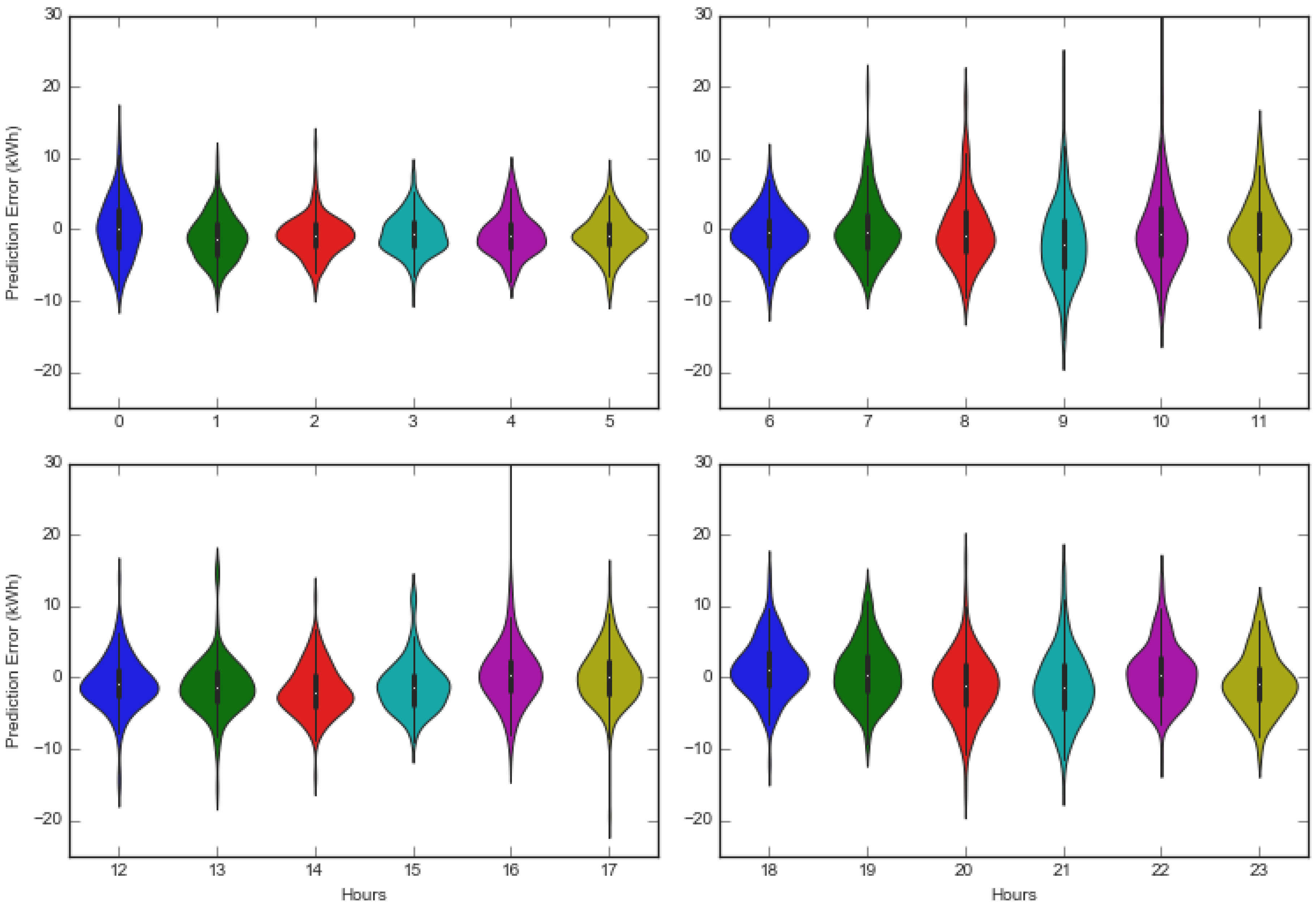
Figure 5 shows the violin plot for probability distribution for extremely randomized model during different hours of the testing dataset. A violin plot is similar to box-and-whisker plot, a box plot indicates variability outside the upper and lower quartiles with a box and whiskers. In a violin plot, the full probability density function in a mirrored form is presented on a vertical axis [55]. The white circle in the middle of the plot indicates median, and the upper and lower ends of the box inside the violin plot indicates the quartiles. In a violin plot, a long slender shape (e.g., such as for hour 9:00 a.m in Figure 5) indicates a large variation and therefore uncertainty in prediction. Short, wide shapes (e.g., hour 2:00 a.m in Figure 5) indicates low variance and concentrated probability mass. The violin charts in Figure 5 show that there is large variation for prediction error during the early morning and late afternoon (4:00 p.m.–5:00 p.m.).

5. Conclusions

Deep learning has shown promising learning and prediction capabilities for different applications. On the other hand, ensemble-based methods were recently developed to overcome problems in traditional methods (e.g., decision trees). This study proposed three machine learning methods to predict hourly HVAC energy consumption of a hotel. Notably, it presented the use of deep highway network—a deep learning method, extra trees—a tree-based ensemble method and a most widely used support vector regression. The paper compared their performance in terms of accuracy and computational efficiency. The analysis performed showed that all three methods have nearly comparable performances. Therefore, the proposed models can achieve accurate and reliable hourly prediction of HVAC energy consumption. The developed models can be used for demand-side management, optimal control and scheduling of HVAC systems, fault detection and diagnosis and predicting behaviour of energy system to mitigate potential uncertainties in smart grids. One of the aspects of this research was to find an answer as to whether deep learning is suitable for predicting high-resolution energy consumption or not. As DHN performed marginally better than the other two studied algorithms; for this problem, it may not be a favourable solution (considering the effort and time required number of different hyperparameters). As from DHN results, it was found that the network complexity did not significantly improve the model’s performance. Therefore, some remaining aspects to reflect on are to investigate the possible reasons in more details i.e., whether (1) the obtained performance is optimal and no further improvements could be achieved; (2) the network complexity has been increased enough to show significant changes in the performance; (3) some variables of interest are missing; and (4) enough historical data is used to ensure the reliable training of a deep learning model. These aspects will be further investigated in the future.

Author Contributions

M.A. and A.M. conceived and designed the experiments; M.Ah. and A.M. performed the experiments; M.A., A.M., Y.R. and M.M. anlysed and interpreted the results; and M.A., A.M., Y.R. and M.M. authors contributed towards writing the paper.

Funding

The work was carried out in the framework of the FP7 project (Grant No. 609154) PERFORMER “Portable, Exhaustive, Reliable, Flexible and Optimized approach to Monitoring and Evaluation of building energy performance” and Horizon 2020 project (Grant No. 731125) PENTAGON “Unlocking European grid local flexibility through augmented energy conversion capabilities at district-level”. The authors acknowledge the financial support from the European Commission.

Conflicts of Interest

The authors declare no conflict of interest. The funding sponsors had no role in the design of the study; in the collection, analyses, or interpretation of data; in the writing of the manuscript, and in the decision to publish the results.

References

  1. Ahmad, M.W.; Mourshed, M.; Mundow, D.; Sisinni, M.; Rezgui, Y. Building energy metering and environmental monitoring— A state-of-the-art review and directions for future research. Energy Build. 2016, 120, 85–102. [Google Scholar] [CrossRef]
  2. Ponta, L.; Raberto, M.; Teglio, A.; Cincotti, S. An Agent-based Stock-flow Consistent Model of the Sustainable Transition in the Energy Sector. Ecol. Econ. 2018, 145, 274–300. [Google Scholar] [CrossRef] [Green Version]
  3. Ahmad, M.W.; Mourshed, M.; Rezgui, Y. Trees vs Neurons: Comparison between random forest and ANN for high-resolution prediction of building energy consumption. Energy Build. 2017, 147, 77–89. [Google Scholar] [CrossRef]
  4. Pérez-Lombard, L.; Ortiz, J.; Pout, C. A review on buildings energy consumption information. Energy Build. 2008, 40, 394–398. [Google Scholar] [CrossRef]
  5. Dascalaki, E.; Balaras, C.A. XENIOS—A methodology for assessing refurbishment scenarios and the potential of application of RES and RUE in hotels. Energy Build. 2004, 36, 1091–1105. [Google Scholar] [CrossRef]
  6. Sloan, P.; Legrand, W.; Chen, J.S. (Eds.) Chapter 2—Energy Efficiency. In Sustainability in the Hospitality Industry; Butterworth-Heinemann: Boston, MA, USA, 2009; pp. 13–26. [Google Scholar]
  7. de Wilde, P. The gap between predicted and measured energy performance of buildings: A framework for investigation. Autom. Constr. 2014, 41, 40–49. [Google Scholar] [CrossRef]
  8. Meyers, R.J.; Williams, E.D.; Matthews, H.S. Scoping the potential of monitoring and control technologies to reduce energy use in homes. Energy Build. 2010, 42, 563–569. [Google Scholar] [CrossRef]
  9. Reddy, T.A. Literature Review on Calibration of Building Energy Simulation Programs: Uses, Problems, Procedures, Uncertainty, and Tools. ASHRAE Trans. 2006, 112, 226. [Google Scholar]
  10. Raftery, P.; Keane, M.; O’Donnell, J. Calibrating whole building energy models: An evidence-based methodology. Energy Build. 2011, 43, 2356–2364. [Google Scholar] [CrossRef]
  11. Ahmad, M.W.; Mourshed, M.; Yuce, B.; Rezgui, Y. Computational intelligence techniques for HVAC systems: A review. Build. Simul. 2016, 9, 359–398. [Google Scholar] [CrossRef] [Green Version]
  12. Manfren, M.; Aste, N.; Moshksar, R. Calibration and uncertainty analysis for computer models—A meta-model based approach for integrated building energy simulation. Appl. Energy 2013, 103, 627–641. [Google Scholar] [CrossRef]
  13. Brea, J.; Senn, W.; Pfister, J.P. Matching Recall and Storage in Sequence Learning with Spiking Neural Networks. J. Neurosci. 2013, 33, 9565–9575. [Google Scholar] [CrossRef] [PubMed] [Green Version]
  14. Diehl, P.U.; Neil, D.; Binas, J.; Cook, M.; Liu, S.C.; Pfeiffer, M. Fast-classifying, high-accuracy spiking deep networks through weight and threshold balancing. In Proceedings of the 2015 IEEE International Joint Conference on Neural Networks (IJCNN), Killarney, UK, 12–16 July 2015; pp. 1–8. [Google Scholar]
  15. He, K.; Zhang, X.; Ren, S.; Sun, J. Delving deep into rectifiers: Surpassing human-level performance on imagenet classification. arXiv, 2015; arXiv:1502.01852. [Google Scholar]
  16. LeCun, Y.; Bengio, Y.; Hinton, G. Deep learning. Nature 2015, 521, 436–444. [Google Scholar] [CrossRef] [PubMed]
  17. Gers, F.A.; Schmidhuber, J.; Cummins, F.A. Learning to forget: Continual prediction with LSTM. In Proceedings of the 9th International Conference on Artificial Neural Networks (ICANN ’99), Edinburgh, UK, 7–10 September 1999. [Google Scholar]
  18. Shi, X.; Chen, Z.; Wang, H.; Yeung, D.; Wong, W.; Woo, W. Convolutional LSTM Network: A Machine Learning Approach for Precipitation Nowcasting. arXiv, 2015; arXiv:1506.04214. [Google Scholar]
  19. Esteva, A.; Kuprel, B.; Novoa, R.A.; Ko, J.; Swetter, S.M.; Blau, H.M.; Thrun, S. Dermatologist-level classification of skin cancer with deep neural networks. Nature 2017, 542, 115. [Google Scholar] [CrossRef] [PubMed]
  20. McCann, B.; Keskar, N.S.; Xiong, C.; Socher, R. The natural language decathlon: Multitask learning as question answering. arXiv, 2018; arXiv:1806.08730. [Google Scholar]
  21. Mnih, V.; Kavukcuoglu, K.; Silver, D.; Rusu, A.A.; Veness, J.; Bellemare, M.G.; Graves, A.; Riedmiller, M.; Fidjeland, A.K.; Ostrovski, G.; et al. Human-level control through deep reinforcement learning. Nature 2015, 518, 529. [Google Scholar] [CrossRef] [PubMed]
  22. Yıldırım, Ö.; Pławiak, P.; Tan, R.S.; Acharya, U.R. Arrhythmia detection using deep convolutional neural network with long duration ECG signals. Comput. Biol. Med. 2018, 102, 411–420. [Google Scholar] [CrossRef] [PubMed]
  23. He, K.; Zhang, X.; Ren, S.; Sun, J. Deep Residual Learning for Image Recognition. arXiv, 2015; arXiv:1512.03385. [Google Scholar]
  24. Chollet, F. Xception: Deep Learning with Depthwise Separable Convolutions. arXiv, 2017; arXiv:1610.02357. [Google Scholar]
  25. Srivastava, R.K.; Greff, K.; Schmidhuber, J. Highway Networks. arXiv, 2015; arXiv:1505.00387. [Google Scholar]
  26. Mocanu, E.; Nguyen, P.H.; Gibescu, M.; Kling, W.L. Deep learning for estimating building energy consumption. Sustain. Energy Grids Netw. 2016. [Google Scholar] [CrossRef]
  27. Marino, D.L.; Amarasinghe, K.; Manic, M. Building Energy Load Forecasting using Deep Neural Networks. In Proceedings of the 42nd IEEE Annual Conference of the IEEE Industrial Electronics Society (IECON), Florence, Italy, 24–27 October 2016. [Google Scholar]
  28. Li, C.; Ding, Z.; Zhao, D.; Zhang, J.Y.G. Building Energy Consumption Prediction: An Extreme Deep Learning Approach. Erngies 2017, 10, 1525. [Google Scholar] [CrossRef]
  29. Mouraud, A. Innovative time series forecasting: auto regressive moving average vs deep networks. Entrep. Sustain. Issues 2017, 4, 282–293. [Google Scholar] [CrossRef] [Green Version]
  30. Mocanu, E.; Mocanu, D.C.; Nguyen, P.H.; Liotta, A.; Webber, M.E.; Gibescu, M.; Slootweg, J. On-Line Building Energy Optimization using Deep Reinforcement Learning. arXiv, 2017; arXiv:1707.05878. [Google Scholar]
  31. Fan, C.; Xiao, F.; Zha, Y. A short-term building cooling load prediction method using deep learning algorithms. Appl. Energy 2017, 195, 222–233. [Google Scholar] [CrossRef]
  32. Liang, J.; Du, R. Model-based Fault Detection and Diagnosis of HVAC systems using Support Vector Machine method. Int. J. Refrig. 2007, 30, 1104–1114. [Google Scholar] [CrossRef]
  33. Mohandes, M.A.; Halawani, T.O.; Rehman, S.; Hussain, A.A. Support vector machines for wind speed prediction. Renew. Energy 2004, 29, 939–947. [Google Scholar] [CrossRef]
  34. Esen, H.; Inalli, M.; Sengur, A.; Esen, M. Modeling a ground-coupled heat pump system by a support vector machine. Renew. Energy 2008, 33, 1814–1823. [Google Scholar] [CrossRef]
  35. Dong, B.; Cao, C.; Lee, S.E. Applying support vector machines to predict building energy consumption in tropical region. Energy Build. 2005, 37, 545–553. [Google Scholar] [CrossRef]
  36. Li, Q.; Meng, Q.; Cai, J.; Yoshino, H.; Mochida, A. Applying support vector machine to predict hourly cooling load in the building. Appl. Energy 2009, 86, 2249–2256. [Google Scholar] [CrossRef]
  37. Li, Q.; Meng, Q.; Cai, J.; Yoshino, H.; Mochida, A. Predicting hourly cooling load in the building: A comparison of support vector machine and different artificial neural networks. Energy Convers. Manag. 2009, 50, 90–96. [Google Scholar] [CrossRef]
  38. Li, X.; Deng, Y.; Ding, L.; Jiang, L. Building cooling load forecasting using fuzzy support vector machine and fuzzy C-mean clustering. In Proceedings of the 2010 International Conference On Computer and Communication Technologies in Agriculture Engineering (CCTAE), Chengdu, China, 12–13 June 2010; Volume 1, pp. 438–441. [Google Scholar]
  39. Yu, Z.; Haghighat, F.; Fung, B.C.; Yoshino, H. A decision tree method for building energy demand modeling. Energy Build. 2010, 42, 1637–1646. [Google Scholar] [CrossRef] [Green Version]
  40. Hong, T.; Koo, C.; Jeong, K. A decision support model for reducing electric energy consumption in elementary school facilities. Appl. Energy 2012, 95, 253–266. [Google Scholar] [CrossRef]
  41. Hong, T.; Koo, C.; Park, S. A decision support model for improving a multi-family housing complex based on CO2 emission from gas energy consumption. Build. Environ. 2012, 52, 142–151. [Google Scholar] [CrossRef]
  42. Tso, G.K.; Yau, K.K. Predicting electricity energy consumption: A comparison of regression analysis, decision tree and neural networks. Energy 2007, 32, 1761–1768. [Google Scholar] [CrossRef]
  43. Vapnik, V. The Nature of Statistical Learning Theory; Springer: New York, NY, USA, 1995. [Google Scholar]
  44. Ahmad, M.W.; Reynolds, J.; Rezgui, Y. Predictive modelling for solar thermal energy systems: A comparison of support vector regression, random forest, extra trees and regression trees. J. Clean. Prod. 2018, 203, 810–821. [Google Scholar] [CrossRef]
  45. Ahmad, M.W.; Mourshed, M.; Rezgui, Y. Tree-based ensemble methods for predicting PV power generation and their comparison with support vector regression. Energy 2018, 164, 465–474. [Google Scholar] [CrossRef]
  46. He, K.; Zhang, X.; Ren, S.; Sun, J. Identity Mappings in Deep Residual Networks. In Computer Vision—ECCV 2016; Leibe, B., Matas, J., Sebe, N., Welling, M., Eds.; Springer: Cham, Switzerland, 2016; pp. 630–645. [Google Scholar]
  47. Glorot, X.; Bordes, A.; Bengio, Y. Deep sparse rectifier neural networks. In Proceedings of the Fourteenth International Conference on Artificial Intelligence and Statistics, Ft. Lauderdale, FL, USA, 11–13 April 2011; pp. 315–323. [Google Scholar]
  48. Geurts, P.; Ernst, D.; Wehenkel, L. Extremely randomized trees. Mach. Learn. 2006, 63, 3–42. [Google Scholar] [CrossRef] [Green Version]
  49. Scalzo, F.; Xu, P.; Asgari, S.; Bergsneider, M.; Hu, X. Regression analysis for peak designation in pulsatile pressure signals. Med. Biol. Eng. Comput. 2009, 47, 967–977. [Google Scholar] [CrossRef] [PubMed] [Green Version]
  50. Nattee, C.; Khamsemanan, N.; Lawtrakul, L.; Toochinda, P.; Hannongbua, S. A novel prediction approach for antimalarial activities of Trimethoprim, Pyrimethamine, and Cycloguanil analogues using extremely randomized trees. J. Mol. Gr. Model. 2017, 71, 13–27. [Google Scholar] [CrossRef] [PubMed]
  51. John, V.; Liu, Z.; Guo, C.; Mita, S.; Kidono, K. Real-Time Lane Estimation Using Deep Features and Extra Trees Regression. In Image and Video Technology: 7th Pacific-Rim Symposium, PSIVT 2015, Auckland, New Zealand, November 25–27 2015, Revised Selected Papers; Bräunl, T., McCane, B., Rivera, M., Yu, X., Eds.; Springer: Cham, Switzerland, 2016; pp. 721–733. [Google Scholar] [CrossRef]
  52. Pedregosa, F.; Varoquaux, G.; Gramfort, A.; Michel, V.; Thirion, B.; Grisel, O.; Blondel, M.; Prettenhofer, P.; Weiss, R.; Dubourg, V.; et al. Scikit-learn: Machine learning in Python. J. Mach. Learn. Res. 2011, 12, 2825–2830. [Google Scholar]
  53. Dieleman, S. Highway Networks. Available online: https://github.com/Lasagne/Lasagne/blob/highway_example/examples/Highway%20Networks.ipynb (accessed on 5 November 2018).
  54. Sutskever, I.; Martens, J.; Dahl, G.; Hinton, G. On the importance of initialization and momentum in deep learning. In Proceedings of the 30th International Conference on Machine Learning, Atlanta, GA, USA, 16–21 June 2013; Volume 28, pp. 1139–1147. [Google Scholar]
  55. Carstens, H.; Xia, X.; Yadavalli, S. Low-cost energy meter calibration method for measurement and verification. Appl. Energy 2017, 188, 563–575. [Google Scholar] [CrossRef] [Green Version]
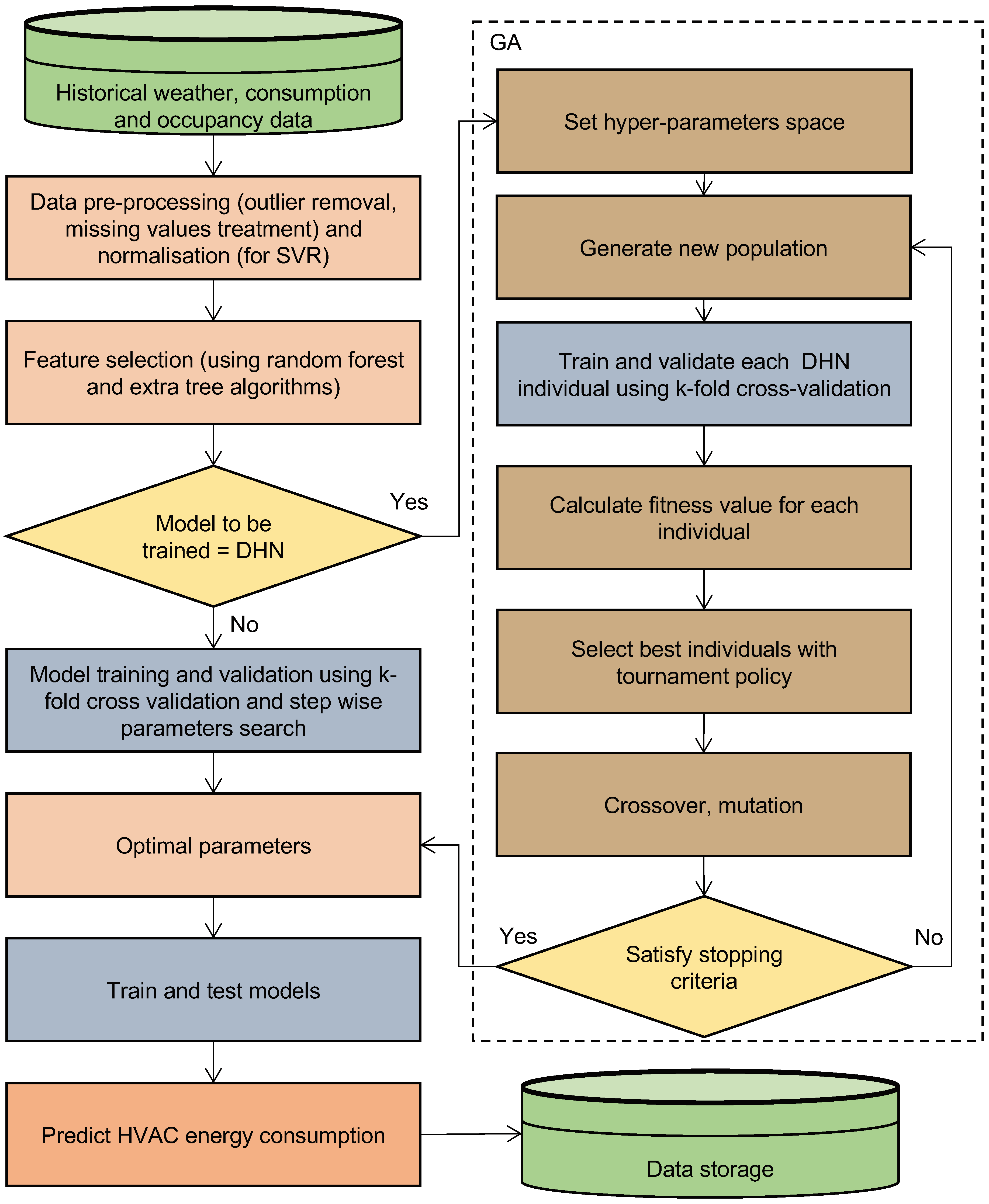
Figure 1. The schematic overview of the proposed research methodology.
Energies 11 03408 g001
Figure 2. Building electricity consumption of (a) a school; (b) a hotel. Reproduced from Ahmad et al. [3], 2017.
Energies 11 03408 g002
Figure 3. Actual hourly HVAC energy consumption. The data shown in the figure is from 15 January 2015 to 15 January 2016.
Energies 11 03408 g003
Figure 4. Results from extremely randomized trees model. (a) comparison between actual and predicted energy consumption from the extremely randomized trees (ET) model; (b) scatter chart illustrating the relationship between predicted and actual energy consumption.
Energies 11 03408 g004
Figure 5. Violin plot showing probability distribution shapes for ET model during different testing hours, with quartiles and median indicated.
Energies 11 03408 g005
Table 1. Summary of the variables used for training and testing.
Input/Output VariablesMinMaxMeanMedian
Outdoor air temperature (°C)−5.540.514.6513
Dew point air temperature (°C)−12204.845
Outdoor air Relative Humidity (%)7.9510058.6958.53
Wind speed (mph)033.656.354.6
No. of rooms booked (-)2311179.5083
No of guests (-)40201124.71127
HVAC hourly energy consumption (kWh)9.3167.847.7840.2
Table 2. Possible values of hyper-parameters defining the space explored by the genetic algorithm.
Decision VariablePossible Values
Number of hidden layer neurons[5, 10, 20, 30]
Number of hidden layers[1, 5, 10, 20, 50]
Epochs[150, 200, 500, 1000, 2000]
Learning Rate[0.005, 0.05, 0.01]
Momentum[0.95, 0.99, 0.995]
Activation function[’VlReLu’, ’Sigmoid’, ’Linear’, ’ReLu’]
Bias[−4.0, −3.0, −2.0, −1.0, 0.0, 1.0]
Model Inputs[[ 1, 1, 1, 2], [1, 1, 1, 24], [24, 24, 1, 24]]
Note: VlReLu: very leaky rectified linear unit; ReLu: Rectified linear units.
Table 3. Top 10 results among the deep highway networks (DHN) models.
Model InputsNumber of NeuronsActivation FunctionNumber of LayersTraining EpochsBiasLearning RateMomentumR2NRMSE (%)
[ 24 , 24 , 1 , 24 ] 30 ReLu1150 3.0 0.01 0.95 0.84 6.007
[ 1 , 1 , 1 , 24 ] 20 VlReLu1500 3.0 0.05 0.95 0.8492 6.008
[ 1 , 1 , 1 , 24 ] 10 Linear1500 3.0 0.05 0.95 0.8490 6.011
[ 1 , 1 , 1 , 24 ] 10 Linear1500 1.0 0.05 0.95 0.8490 6.013
[ 1 , 1 , 1 , 24 ] 5 Linear1500 3.0 0.05 0.95 0.8489 6.014
[ 1 , 1 , 1 , 24 ] 20 VlReLu501000 2.0 0.005 0.95 0.8484 6.024
[ 1 , 1 , 1 , 24 ] 5 VlReLu11000 3.0 0.05 0.95 0.8482 6.028
[ 1 , 1 , 1 , 24 ] 5 Linear501000 2.0 0.005 0.95 0.8482 6.029
[ 1 , 1 , 1 , 24 ] 20 Linear20500 1.0 0.005 0.95 0.8481 6.029
[ 1 , 1 , 1 , 24 ] 10 VlReLu11000 3.0 0.05 0.95 0.8481 6.030
[ 1 , 1 , 1 , 24 ] 5 VlReLu502000 2.0 0.05 0.95 0.8481 6.030
The “Model inputs” array is represented as [Outdoor air temperature, Relative humidity, No. of guests, previous hours HVAC energy consumption].
Table 4. Best results among the DHN models with minimal complexity.
Model InputsNumber of NeuronsActivation FunctionNumber of LayersTraining EpochsBiasLearning RateMomentumR2NRMSE (%)
[ 1 , 1 , 1 , 2 ] 10VlReLu11000 0.0 0.05 0.95 0.8444 6.10
[ 1 , 1 , 1 , 2 ] 10ReLu1150 2.0 0.05 0.99 0.8416 6.16
[ 1 , 1 , 1 , 2 ] 30VlReLu1200 4.0 0.05 0.95 0.8431 6.13
[ 1 , 1 , 1 , 24 ] 5Linear1500 3.0 0.05 0.95 0.8489 6.014
[ 1 , 1 , 1 , 24 ] 5Linear1200 2.0 0.005 0.95 0.8445 6.10
[ 1 , 1 , 1 , 24 ] 5ReLu11000 1.0 0.01 0.95 0.8425 6.14
Table 5. Results of different C, where ϵ = 0.1.
CR2 (–)RMSE (kWh)MAE (kWh)
2 7 −0.33612.50110.601
2 6 −0.30712.36210.448
2 5 −0.25912.13210.188
2 4 −0.17611.7269.752
2 3 0.02110.7008.795
2 2 0.3808.5186.912
2 1 0.6705.9264.658
2 0 0.8014.8213.644
2 1 0.8294.4723.316
2 2 0.8394.3433.188
2 3 0.8434.2883.123
2 4 0.8444.2743.102
2 5 0.8444.2693.091
2 6 0.8444.2683.088
2 7 0.8444.2693.087
Table 6. Results of different ϵ , where C = 2 5 .
ϵ R2 (–)RMSE (kWh)MAE (kWh)
2 10 0.844274.26753.0924
2 9 0.844284.26733.0922
2 8 0.844294.26713.0920
2 7 0.844274.26743.0922
2 6 0.844214.26823.0928
2 5 0.844164.26903.0927
2 4 0.844184.26863.0916
2 3 0.844264.26753.0903
2 2 0.844534.26393.0881
2 1 0.844674.26193.0849
2 0 0.844774.26063.0877
2 1 0.845364.25253.0896
2 2 0.840274.32193.2041
2 3 0.798784.85083.8013
2 4 0.553417.22676.1642
2 5 −0.4495713.020011.2723
Table 7. Results of different n min , where K = n and M = 1000.
n min R2 (–)RMSE (kWh)MAE (kWh)
20.8194.6013.405
30.8224.5643.377
50.8284.4853.312
70.8324.4273.266
100.8374.3723.223
Table 8. Results of different K, where n min = 3 and M = 1000.
KR2 (–)RMSE (kWh)MAE (kWh)
10.74855.4234.200
20.80914.7243.555
30.82264.5553.385
40.82464.5293.353
50.82194.5643.377
Table 9. Results of different d max , where n min = 3, K = 4 and M = 1000.
d max R2 (–)RMSE (kWh)MAE (kWh)
1−0.324212.44510.578
30.53237.3966.128
50.76295.2654.199
70.82814.4843.413
90.84244.2923.184
100.84274.2883.167
150.83534.3893.227
200.82624.5083.331
Table 10. Comparison of extremely randomized trees (ET), support vector regression (SVR) and deep highway network (DHN) models.
ModelTraining DatasetTesting Dataset
RMSE (kWh)R2 (–)RMSE (kWh)MAE (kWh)
ET4.2840.84274.2883.167
SVR4.2520.84534.2533.090
DHN3.0870.84914.2003.027
Table 11. Statistical measures on testing dataset for DHN, ET and SVR.
Factor/VariableActual E.C. DataDHNETSVR
Mean37.0837.1637.4837.09
Median35.235.4635.8835.68
Standard Deviation10.829.889.519.82
Sample Variance116.9897.6890.5196.51
Kurtosis1.140.621.100.97
Skewness0.960.820.930.88
Range69.9064.3058.2563.88
Minimum17.216.8422.8718.31
Maximum87.181.1481.1282.19
Sum121,981.7122,245.60123,308.75122,015.85