Investigating the Predictive Performance of Gaussian Process Regression in Evaluating Reservoir Porosity and Permeability


 ,
,
Abstract
1. Introduction
2. Data and Methods
2.1. Data Description
2.2. Gaussian Process Regression
- Matern 3/2:
- Matern 5/2:
- Exponential:
- Rational quadratic:
3. Results
3.1. Developing GPR Models
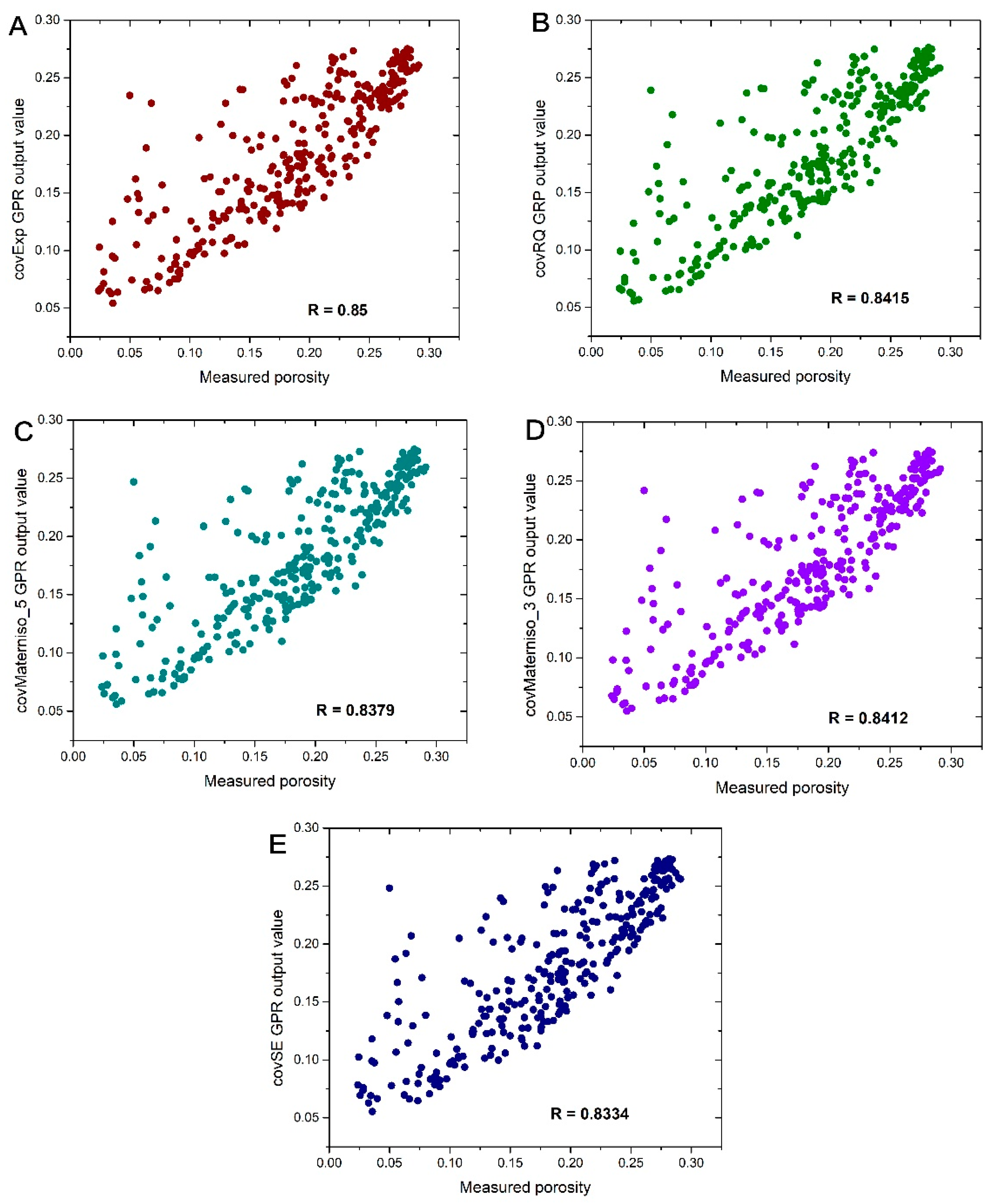
3.2. Performance of Porosity Models
3.3. Performance of Permeability Models
3.4. Comparative Analysis with Artificial Neural Network (ANN)
3.5. Comparing CovExp-GPR Porosity Results with ANN
3.6. Comparing Permeability Results with ANN
4. Conclusions
Author Contributions
Funding
Conflicts of Interest
References
- Ehsan, M.; Gu, H.; Akhtar, M.M.; Abbasi, S.S.; Ullah, Z. Identification of Hydrocarbon Potential of Talhar Shale: Member of Lower Goru Formation by Using Well Logs Derived Parameters, Southern Lower Indus Basin, Pakistan. J. Earth Sci. 2018, 29, 587–593. [Google Scholar] [CrossRef]
- Gao, D.; Cheng, R.; Shen, Y.; Wang, L.; Hu, X. Weathered and Volcanic Provenance-Sedimentary System and Its Influence on Reservoir Quality in the East of the Eastern Depression, the North Yellow Sea Basin. J. Earth Sci. 2018, 29, 353–368. [Google Scholar] [CrossRef]
- Mohaghegh, S.; Arefi, R.; Ameri, S.; Aminiand, K.; Nutter, R. Petroleum reservoir characterization with the aid of artificial neural networks. J. Pet. Sci. Eng. 1996, 16, 263–274. [Google Scholar] [CrossRef]
- Anifowose, F.A.; Labadin, J.; Abdulraheem, A. Hybrid intelligent systems in petroleum reservoir characterization and modeling: The journey so far and the challenges ahead. J. Pet. Explor. Prod. Technol. 2017, 7, 251–263. [Google Scholar] [CrossRef]
- Karimpouli, S.; Fathianpour, N.; Roohi, J. A new approach to improve neural networks’ algorithm in permeability prediction of petroleum reservoirs using supervised committee machine neural network (SCMNN). J. Pet. Sci. Eng. 2010, 73, 227–232. [Google Scholar] [CrossRef]
- Iturrarán-Viveros, U.; Parra, J.O. Artificial Neural Networks applied to estimate permeability, porosity and intrinsic attenuation using seismic attributes and well-log data. J. Appl. Geophys. 2014, 107, 45–54. [Google Scholar] [CrossRef]
- Bagheripour, P. Committee Neural Network Model for Rock Permeability Prediction. J. Appl. Geophys. 2014, 104, 142–148. [Google Scholar] [CrossRef]
- Na’imi, S.R.; Shadizadeh, S.R.; Riahi, M.A.; Mirzakhanian, M. Estimation of Reservoir Porosity and Water Saturation Based on Seismic Attributes Using Support Vector Regression Approach. J. Appl. Geophys. 2014, 107, 93–101. [Google Scholar] [CrossRef]
- Plastino, A.; Gonçalves, E.C.; da Silva, P.N.; Carneiro, G.; Azeredo, R.B. Combining Classification and Regression for Improving Permeability Estimations from 1H-NMR Relaxation Data. J. Appl. Geophys. 2017, 146, 95–102. [Google Scholar] [CrossRef]
- Anifowose, F.; Abdulraheem, A. Fuzzy logic-driven and SVM-driven hybrid computational intelligence models applied to oil and gas reservoir characterization. J. Nat. Gas Sci. Eng. 2011, 3, 505–517. [Google Scholar] [CrossRef]
- Helmy, T.; Fatai, A.; Faisal, K. Hybrid computational models for the characterization of oil and gas reservoirs. Expert Syst. Appl. 2010, 37, 5353–5363. [Google Scholar] [CrossRef]
- Anifowose, F.; Labadin, J.; Abdulraheem, A. Improving the prediction of petroleum reservoir characterization with a stacked generalization ensemble model of support vector machines. Appl. Soft Comput. 2015, 26, 483–496. [Google Scholar] [CrossRef]
- Ali, D.; Ebrahim, S. Physical properties modeling of reservoirs in Mansuri oil field, Zagros region, Iran. Pet. Explor. Dev. 2016, 43, 611–615. [Google Scholar] [CrossRef]
- Baziar, S.; Tadayoni, M.; Nabi-Bidhendi, M.; Khalili, M. Prediction of permeability in a tight gas reservoir by using three soft computing approaches: A comparative study. J. Nat. Gas Sci. Eng. 2014, 21, 718–724. [Google Scholar] [CrossRef]
- Yu, H.; Wang, Z.; Rezaee, R.; Zhang, Y.; Xiao, L.; Luo, X.; Wang, X.; Zhang, L. The Gaussian Process Regression for TOC Estimation Using Wireline Logs in Shale Gas Reservoirs. In Proceedings of the International Petroleum Technology Conference, Bangkok, Thailand, 14–16 November 2016. [Google Scholar] [CrossRef]
- Aye, S.A.; Heyns, P.S. An integrated Gaussian process regression for prediction of remaining useful life of slow speed bearings based on acoustic emission. Mech. Syst. Signal Process. 2017, 84, 485–498. [Google Scholar] [CrossRef]
- Bishop, C.M. Pattern Recognition and Machine Learning; Springer: New York, NY, USA, 2006. [Google Scholar]
- Richardson, R.R.; Osborne, M.A.; Howey, D.A. Gaussian process regression for forecasting battery state of health. J. Power Sources 2017, 357, 209–219. [Google Scholar] [CrossRef]
- Heyns, T.; de Villiers, J.P.; Heyns, P.S. Consistent haul road condition monitoring by means of vehicle response normalisation with Gaussian processes. Eng. Appl. Artif. Intell. 2012, 25, 1752–1760. [Google Scholar] [CrossRef]
- Rawlinson, A.A.; Vasudevan, S. Gaussian Process Modeling of Well Logs. In Proceedings of the IEEE European Modelling Symposium, Madrid, Spain, 6–8 October 2015. [Google Scholar] [CrossRef]
- Yi, S.; Yi, S.; Batten, D.J.; Yun, H.; Park, S.J. Cretaceous and Cenozoic non-marine deposits of the Northern South Yellow Sea Basin, offshore western Korea: Palynostratigraphy and palaeoenvironments. Palaeogeogr. Palaeoclimatol. Palaeoecol. 2003, 191, 15–44. [Google Scholar] [CrossRef]
- Wu, S.; Ni, X.; Cai, F. Petroleum geological framework and hydrocarbon potential in the Yellow Sea. Chin. J. Oceanol. Limnol. 2008, 26, 23–34. [Google Scholar] [CrossRef]
- Pang, Y.; Zhang, X.; Xiao, G.; Wen, Z.; Guo, X.; Hou, F.; Zhu, X. Structural and geological characteristics of the South Yellow Sea Basin in Lower Yangtze Block. Geol. Rev. 2016, 62, 604–616. (In Chinese) [Google Scholar]
- Fang, D.; Zhang, X.; Yu, Q.; Jin, T.C.; Tian, L. A novel method for carbon dioxide emission forecasting based on improved Gaussian processes regression. J. Clean. Prod. 2018, 173, 143–150. [Google Scholar] [CrossRef]
- Kong, D.; Chen, Y.; Li, N. Gaussian process regression for tool wear prediction. Mech. Syst. Signal Process. 2018, 104, 556–574. [Google Scholar] [CrossRef]
- Rasmussen, C.E.; Williams, C.K.I. Gaussian Processes for Machine Learning; The MIT Press: Cambridge, MA, USA; London, UK, 2006. [Google Scholar]
- Brantson, E.T.; Ju, B.; Ziggah, Y.Y.; Akwensi, P.H.; Sun, Y.; Wu, D.; Addo, B.J. Forecasting of Horizontal Gas Well Production Decline in Unconventional Reservoirs using Productivity, Soft Computing and Swarm Intelligence Models. Nat. Resour. Res. 2018. [Google Scholar] [CrossRef]


| Well A | GR (api) | DT (μs/m) | RT (Ωm) | SP (mv) | Porosity | Permeability (mD) |
|---|---|---|---|---|---|---|
| Min | 33.845 | 59.979 | 0.73 | 349.496 | 0.02411 | 0.001 |
| Max | 89.872 | 147.332 | 13.721 | 387.145 | 0.29478 | 59.874 |
| Mean | 65.364 | 103.016 | 2.166 | 365.827 | 0.17498 | 9.2888 |
| SD | 15.431 | 11.648 | 0.924 | 10.885 | 0.07152 | 11.1292 |
| Well B | GR (api) | DT (μs/m) | RT (Ωm) | SP (mv) | Porosity | Permeability (mD) |
|---|---|---|---|---|---|---|
| Min | 36.581 | 56.219 | 0.732 | 348.972 | 0.02378 | 0.001 |
| Max | 89.848 | 142.136 | 5.575 | 387.043 | 0.29117 | 54.216 |
| Mean | 64.046 | 102.618 | 2.187 | 367.356 | 0.18569 | 10.9582 |
| SD | 15.650 | 10.1152 | 0.6498 | 10.731 | 0.07081 | 12.1387 |
| Statistical Index | covSE | covRQ | covMarten 5 | covMatern 3 | covExp |
|---|---|---|---|---|---|
| R | 0.8334 | 0.8415 | 0.8379 | 0.8412 | 0.85 |
| RMSE | 0.0387 | 0.0387 | 0.0387 | 0.0387 | 0.0374 |
| Statistical Index | covSE | covRQ | covMarten 5 | covMatern 3 | covExp |
|---|---|---|---|---|---|
| R | 0.8402 | 0.8428 | 0.8429 | 0.8439 | 0.85 |
| RMSE | 6.5780 | 6.5309 | 6.5295 | 6.5101 | 6.4717 |
| Performance Index | CovExp-GPR | BPNN | GRNN | RBFNN |
|---|---|---|---|---|
| R | 0.85 | 0.84 | 0.86 | 0.86 |
| RMSE | 0.036 | 0.038 | 0.037 | 0.036 |
| Computational time (s) | 22.01 | 265.79 | 29.66 | 96.58 |
| Performance Index | CovExp-GPR | BPNN | GRNN | RBFNN |
|---|---|---|---|---|
| R | 0.85 | 0.86 | 0.86 | 0.85 |
| RMSE | 6.47 | 6.27 | 6.14 | 6.47 |
| Computational time (s) | 20.72 | 190.04 | 28.21 | 100.14 |
© 2018 by the authors. Licensee MDPI, Basel, Switzerland. This article is an open access article distributed under the terms and conditions of the Creative Commons Attribution (CC BY) license (http://creativecommons.org/licenses/by/4.0/).
Share and Cite
Asante-Okyere, S.; Shen, C.; Yevenyo Ziggah, Y.; Moses Rulegeya, M.; Zhu, X. Investigating the Predictive Performance of Gaussian Process Regression in Evaluating Reservoir Porosity and Permeability. Energies 2018, 11, 3261. https://doi.org/10.3390/en11123261
Asante-Okyere S, Shen C, Yevenyo Ziggah Y, Moses Rulegeya M, Zhu X. Investigating the Predictive Performance of Gaussian Process Regression in Evaluating Reservoir Porosity and Permeability. Energies. 2018; 11(12):3261. https://doi.org/10.3390/en11123261
Chicago/Turabian StyleAsante-Okyere, Solomon, Chuanbo Shen, Yao Yevenyo Ziggah, Mercy Moses Rulegeya, and Xiangfeng Zhu. 2018. "Investigating the Predictive Performance of Gaussian Process Regression in Evaluating Reservoir Porosity and Permeability" Energies 11, no. 12: 3261. https://doi.org/10.3390/en11123261
APA StyleAsante-Okyere, S., Shen, C., Yevenyo Ziggah, Y., Moses Rulegeya, M., & Zhu, X. (2018). Investigating the Predictive Performance of Gaussian Process Regression in Evaluating Reservoir Porosity and Permeability. Energies, 11(12), 3261. https://doi.org/10.3390/en11123261