Competing Retailers’ Environmental Investment: An Analysis under Different Power Structures

Abstract
:1. Introduction
2. Literature Review
3. Modeling Framework
- Nash Game (N): the two sites of the supply chain, the manufacturer and the retailers, have the same power. They play a Nash game in which they decide on the wholesale price and carbon emission reduction level through investment and retail price, simultaneously. The optimal decisions are Nash equilibrium in which each firm’s decisions are the best response of the others’ decisions.
- Manufacturer-lead Stackelberg Game (M): The manufacturer is more powerful than the two retailers. Accordingly, it is a Stackelberg game where the manufacturer plays as the leader. We call it M-lead game for short. The decision sequence is as follows: the manufacturer first decides the wholesale price; then, the two retailers decide their own retail price and the emission reduction level to respond to the wholesale price simultaneously.
- Retailer-lead Stackelberg Game (R): The two retailers are more powerful than the manufacturer. It is a Stackelberg game where the retailers are leaders in the supply chain. We call it R-lead game for short. In the decision sequence, the two retailers decide their own emission reduction level through investment and retail price simultaneously. Then, the manufacturer responds by setting the wholesale price.
4. Analysis of Different Power Structures
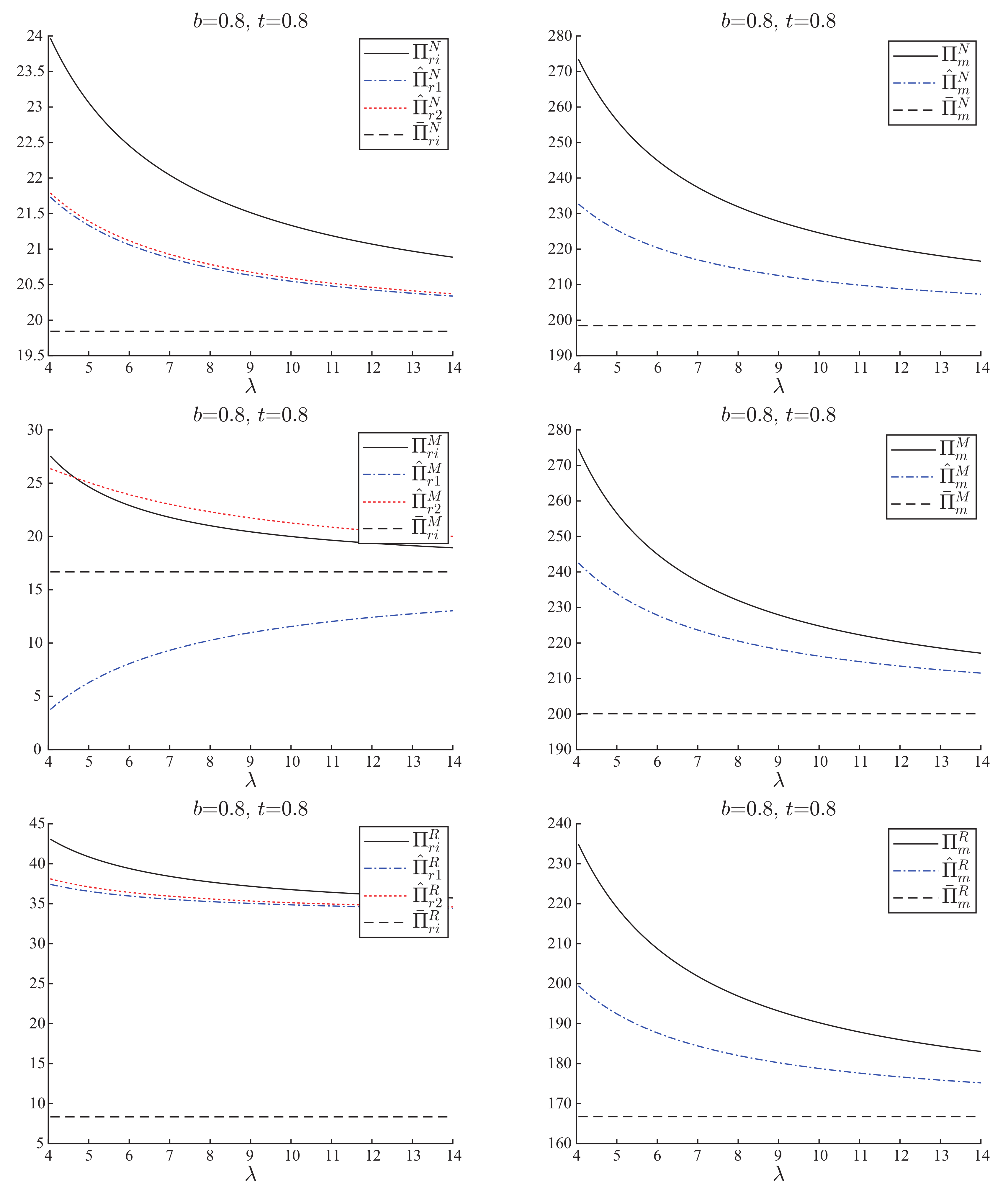
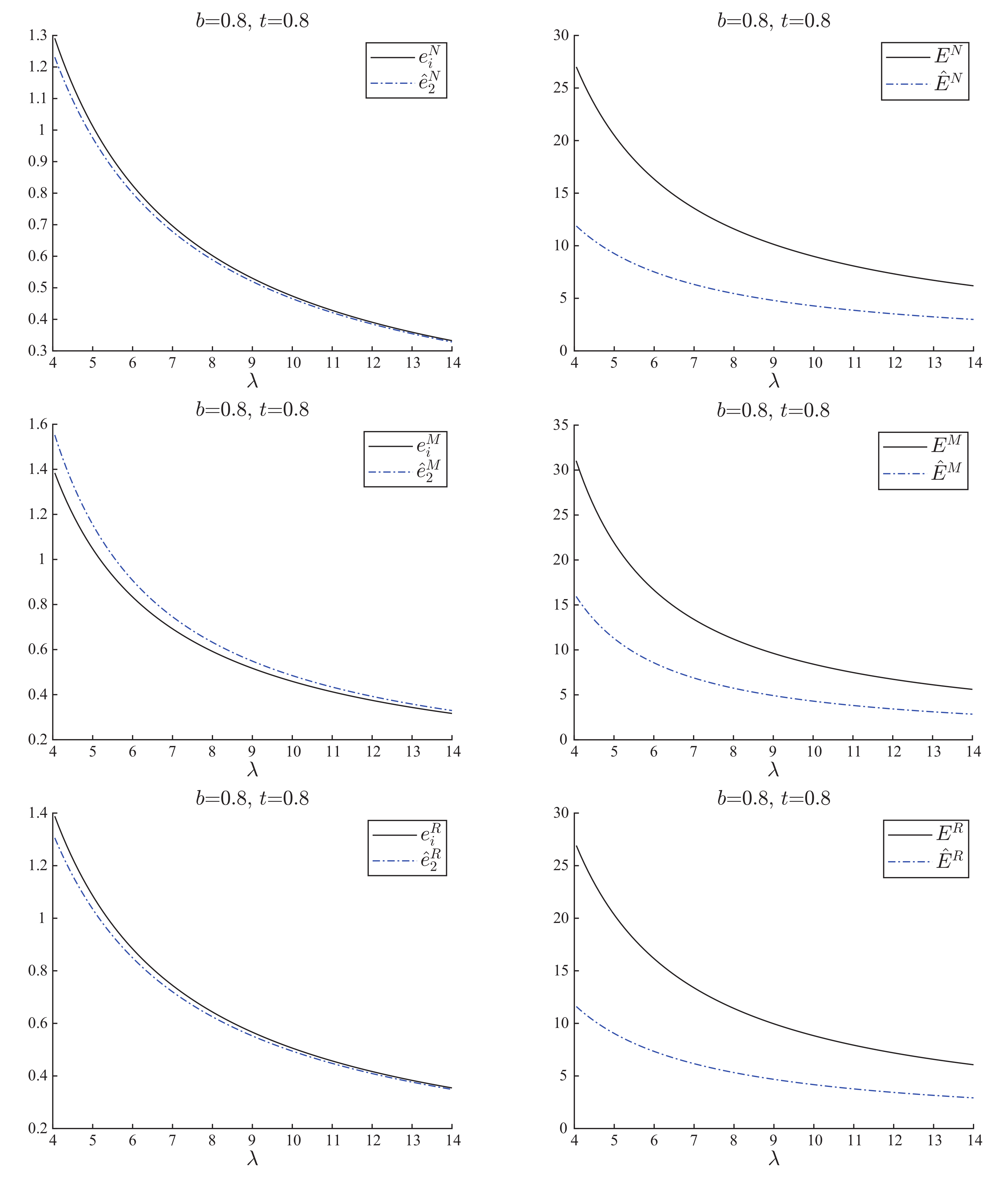
- 1.
- , , are all decreasing in λ.
- 2.
- and are decreasing in λ. is increasing in λ only when .
- 3.
- is increasing in λ only when . is increasing in λ. is increasing in λ only when .
5. Comparison and Insights
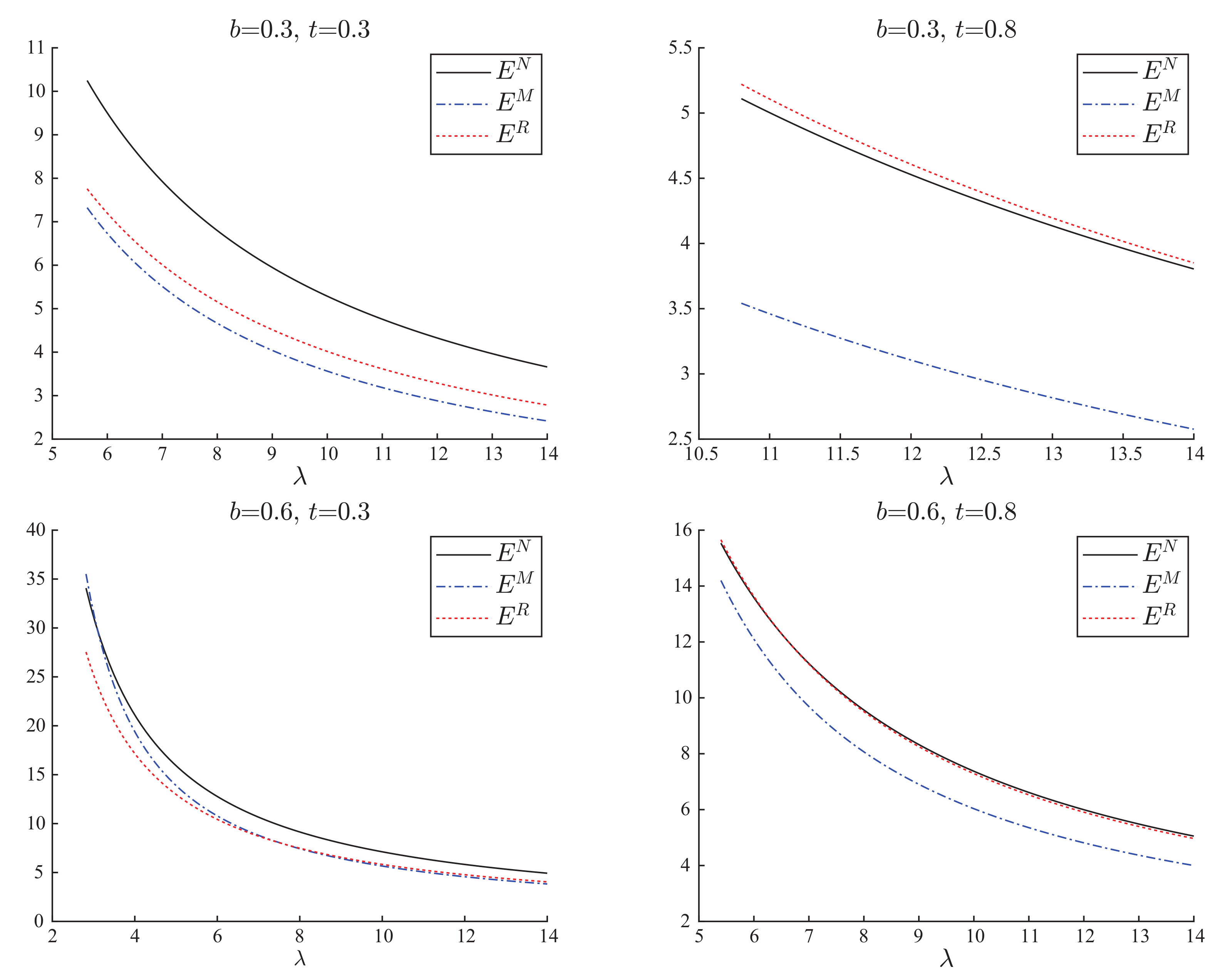
5.1. Incentive of Retailers’ Sustainable Investment in Different Power Structures
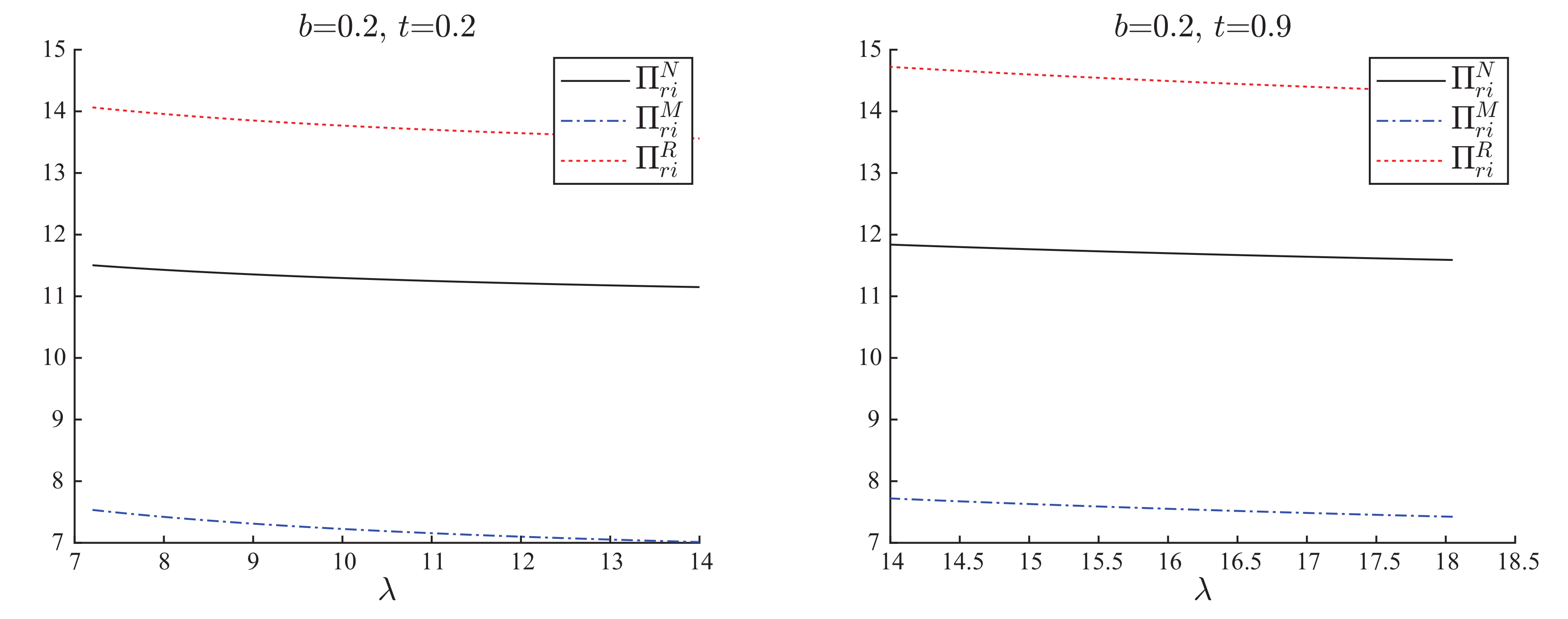
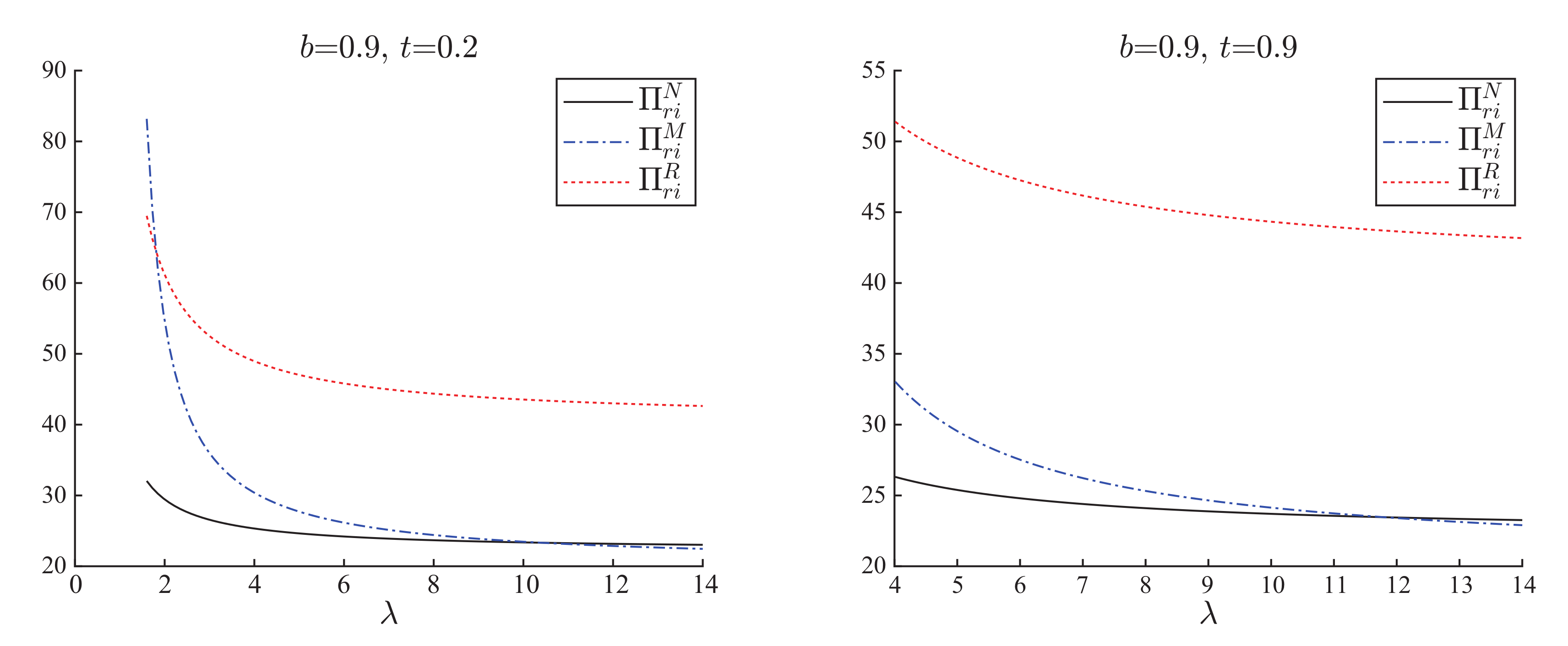
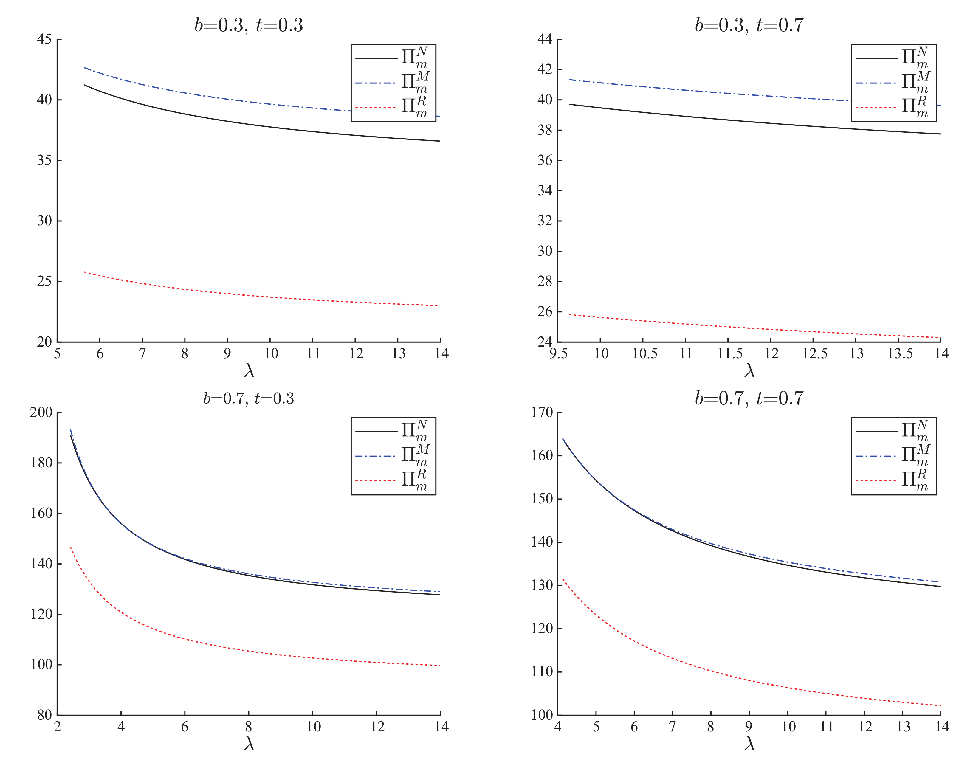
5.2. Impact of Retailers’ Power on Decisions and Performances
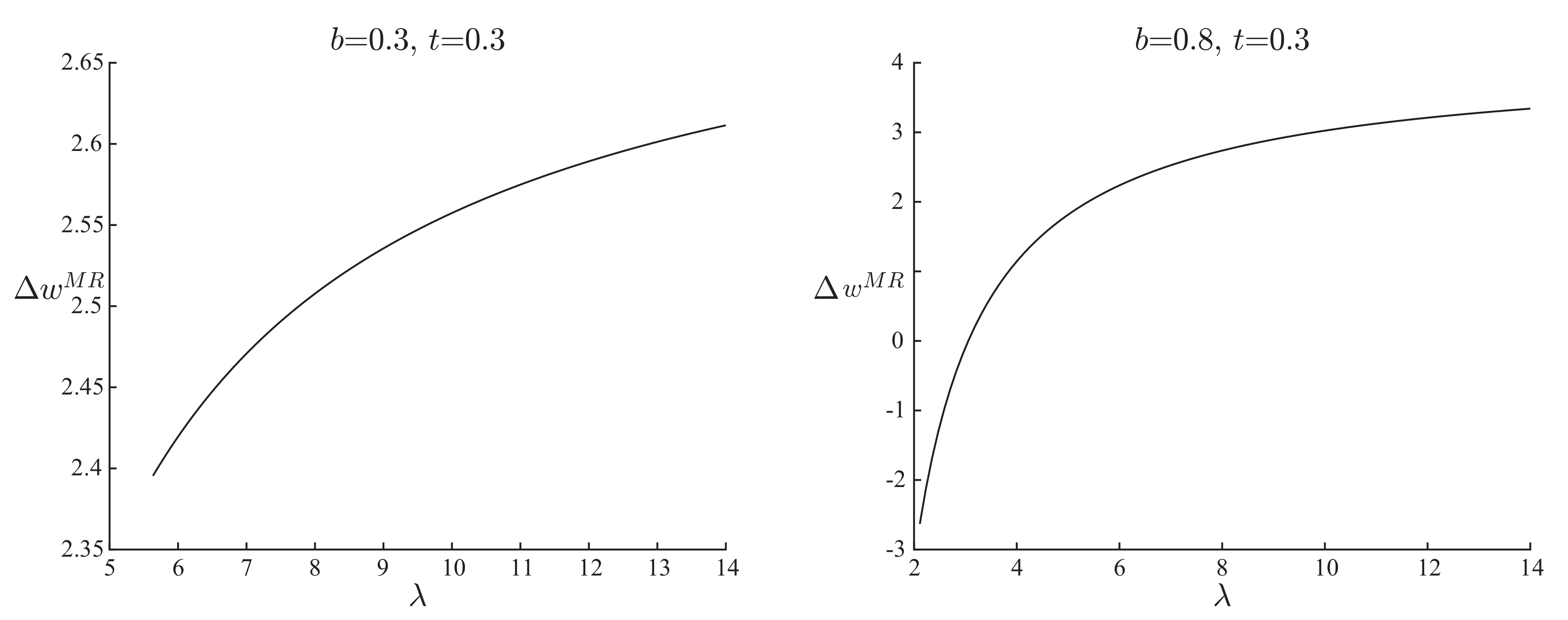
- 1.
- When , ; otherwise, .
- 2.
- When , ; otherwise, .
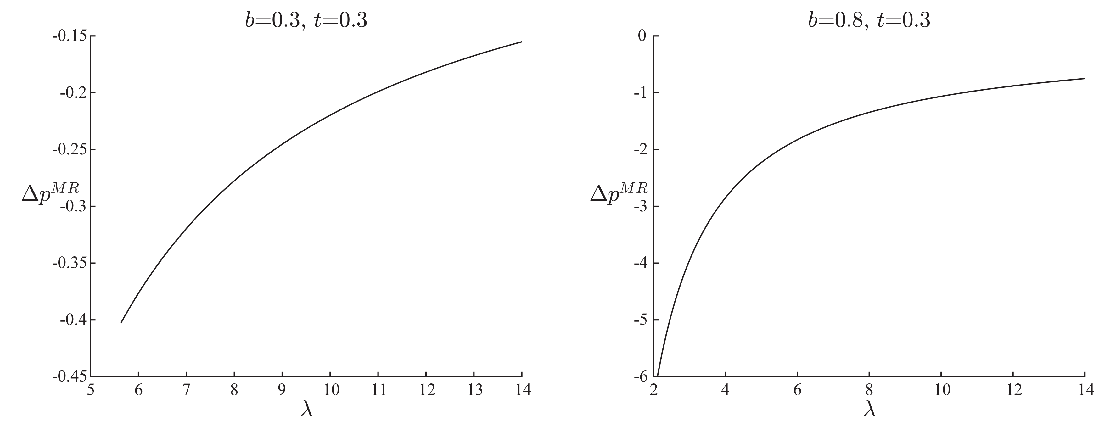
- 3.
- When , ; otherwise, .
5.3. Extension
6. Conclusions
Funding
Conflicts of Interest
Appendix A
- When all the firms have the same power, we solve the three firms’ decisions simultaneously. The first-order derivatives are , , The Hesse matrix of retailer’s profit function isThe Hesse matrix of manufacturer’s profit function isTherefore, we solve the optimal decisions by . Thus, we get , , , , where . Furthermore, it is obvious that and .
- When the manufacturer is more powerful, given the wholesale price, we solve the optimal reduction levels and retail prices of two retailers. The first-order derivatives are , From , we get and . Substituting into the manufacturer’s profit function, we get . We solve the optimal wholesale price by . Thus, we get , , , , where . Furthermore, it is obvious that and .
- When the two retailers are more powerful, given the reduction levels and the retail prices, we first solve the optimal wholesale price. The first-order derivatives are . By solving , we get . Substituting the optimal respond wholesale price into retailers profit functions, we get , . Therefore, we get the optimal decisions by .Thus, we get , , , , where . Furthermore, it is obvious that and .
- Notice that , and are all increasing in . Then, we get , , are all decreasing in .
- The first-order derivative of optimal retail prices in are , , . It is easy to find that and are negative because of . is positive only when .
- The first-order derivative of optimal wholesale prices in are , , . It is easy to find that is positive only when . Because , is positive. By solving the equation in t, we get the solutions are and . Notice that the first solution is negative; therefore, is positive only when .
- The difference between and is . Obviously, the formula is positive only when . The constraint of has been considered in the proof of Proposition 6.
- Notice that . Therefore, it is easy to find that .
- The difference between and is . Obviously, the formula is positive only when . The constraint of has been considered in the proof of Proposition 6.
- The difference between and is . With the assumption , it is obvious that . Therefore, .
- The difference between and is . Obviously, the formula is negative only when . Consider the constraint of ; solving the equation in t, we get only when and .
- The difference between and is . The signal of the formula is independent from . When we get .
- The difference between and is . Obviously, the formula is positive only when .
References
- Krass, D.; Nedorezov, T.; Ovchinnikov, A. Environmental taxes and the choice of green technology. Prod. Oper. Manag.. 2013, 22, 1035–1055. [Google Scholar] [CrossRef]
- Drake, D.F.; Kleindorfer, P.R.; Van Wassenhove, L.N. Technology choice and capacity portfolios under emissions regulation. Prod. Oper. Manag. 2015, 25, 1006–1025. [Google Scholar] [CrossRef]
- Dong, C.; Shen, B.; Chow, P.S.; Yang, L.; Ng, C.T. Sustainability investment under cap-and-trade regulation. Ann. Oper. Res. 2016, 240, 509–531. [Google Scholar] [CrossRef]
- Toptal, A.; Özlü, H.; Konur, D. Joint decisions on inventory replenishment and emission reduction investment under different emission regulations. Int. J. Prod. Res. 2014, 52, 243–269. [Google Scholar] [CrossRef] [Green Version]
- Shi, X.; Qian, Y.; Dong, C. Economic and Environmental Performance of Fashion Supply Chain: The Joint Effect of Power Structure and Sustainable Investment. Sustainability 2017, 9, 961. [Google Scholar] [CrossRef]
- Marks&Spencer Plan A Report 2016. Available online: http://planareport.marksandspencer.com/M&S_PlanA_Report_2016.pdf (accessed on 15 June 2016).
- NIKE Sustainable Business Report 2017. Available online: https://sustainability-nike.s3.amazonaws.com/wp-content/uploads/2018/05/18175102/NIKE-FY1617-Sustainable-Business-Report_FINAL.pdf (accessed on 15 June 2016).
- Du, S.; Zhu, J.; Jiao, H.; Ye, W. Game-theoretical analysis for supply chain with consumer preference to low carbon. Int. J. Prod. Res. 2015, 53, 3753–3768. [Google Scholar] [CrossRef]
- Li, Q.; Shen, B. Sustainable Design Operations in the Supply Chain: Non-Profit Manufacturer vs. For-Profit Manufacturer. Sustainability 2016, 8, 639. [Google Scholar] [CrossRef]
- Yalabik, B.; Fairchild, R.J. Customer, regulatory, and competitive pressure as drivers of environmental innovation. Int. J. Prod. Econ. 2011, 131, 519–527. [Google Scholar] [CrossRef]
- Liu, Z.L.; Anderson, T.D.; Cruz, J.M. Consumer environmental awareness and competition in two-stage supply chains. Eur. J. Oper. Res. 2012, 218, 602–613. [Google Scholar] [CrossRef]
- Zhang, L.; Wang, J.; You, J. Consumer environmental awareness and channel coordination with two substitutable products. Eur. J. Oper. Res. 2015, 241, 63–73. [Google Scholar] [CrossRef]
- Cachon, G.P.; Netessine, S. Game theory in supply chain analysis. In Models, Methods, and Applications for Innovative Decision Making; Johnson, M.P., Norman, B., Secomandi, N., Gray, P., Greenberg, H.J., Eds.; Informs: New York, NY, USA, 2006; pp. 200–233. [Google Scholar]
- Feng, Q.; Lu, X. The strategic perils of low cost out-sourcing. Manage. Sci. 2012, 58, 1196–1210. [Google Scholar] [CrossRef]
- Feng, Q.; Lu, X. The role of contract negotiation and industry structure in production outsourcing. Prod. Oper. Mana. 2013, 22, 1299–1319. [Google Scholar] [CrossRef]
- Anderson, E.J.; Bao, Y. Price competition with integrated and decentralized supply chains. Eur. J. Oper. Res. 2010, 200, 227–234. [Google Scholar] [CrossRef]
- Wang, Z.; Hu, M. Committed versus contingent pricing under competition. Prod. Oper. Manag. 2014, 23, 1919–1936. [Google Scholar] [CrossRef]
- Zhao, X.; Atkins, D.R. Newsvendors under simultaneous price and inventory competition. Manuf. Ser. Oper. Manag. 2008, 10, 539–546. [Google Scholar] [CrossRef]
- Giri, B.C.; Sharma, S. Manufacturer’s pricing strategy in a two-level supply chain with competing retailers and advertising cost dependent demand. Econ. Model. 2014, 38, 102–111. [Google Scholar] [CrossRef]
- Bernstein, F.; Federgruen, A. Pricing and replenishment strategies in a distribution system with competing retailers. Oper. Res. 2003, 51, 409–426. [Google Scholar] [CrossRef]
- Xiao, T.; Qi, X. Price competition, cost and demand disruptions and coordination of a supply chain with one manufacturer and two competing retailers. Omega 2008, 36, 741–753. [Google Scholar] [CrossRef]
- Cao, E.; Wan, C.; Lai, M. Coordination of a supply chain with one manufacturer and multiple competing retailers under simultaneous demand and cost disruptions. Int. J. Prod. Econ. 2013, 141, 425–433. [Google Scholar]
- Ertek, G.; Griffin, P.M. Supplier-and buyer-driven channels in a two-stage supply chain. IIE Trans. 2002, 34, 691–700. [Google Scholar] [CrossRef]
- Majumder, P.; Srinivasan, A. Leader location, cooperation, and coordination in serial supply chains. Prod. Oper. Manag. 2006, 15, 22. [Google Scholar]
- Xue, W.; Demirag, O.C.; Niu, B. Supply chain performance and consumer surplus under alternative structures of channel dominance. Eur. J. Oper. Res. 2014, 239, 130–145. [Google Scholar] [CrossRef]
- Shi, R.; Zhang, J.; Ru, J. Impacts of power structure on supply chains with uncertain demand. Prod. Oper. Manag. 2013, 22, 1232–1249. [Google Scholar] [CrossRef]
- Choi, S.C. Price competition in a channel structure with a common retailer. Market. Sci. 1991, 10, 271–296. [Google Scholar] [CrossRef]
- Chen, X.; Wang, X.; Jiang, X. The impact of power structure on the retail service supply chain with an O2O mixed channel. J. Oper. Res. Soc. 2016, 67, 294–301. [Google Scholar] [CrossRef]
- Zheng, B.; Yang, C.; Yang, J.; Zhang, M. Dual-channel closed loop supply chains: Forward channel competition, power structures and coordination. Int. J. Prod. Res. 2017, 1–18. [Google Scholar] [CrossRef]
- Chen, X.; Wang, X.; Chan, H.K. Manufacturer and retailer coordination for environmental and economic competitiveness: A power perspective. Trans. Res. Part E Logist. Trans. Rev. 2017, 97, 268–281. [Google Scholar] [CrossRef] [Green Version]
- Shi, X.; Zhang, X.; Dong, C.; Wen, S. Economic Performance and Emission Reduction of Supply Chains in Different Power Structures: Perspective of Sustainable Investment. Energies 2018, 11, 983. [Google Scholar] [CrossRef]
- Cai, G.G.; Zhang, Z.G.; Zhang, M. Game theoretical perspectives on dual-channel supply chain competition with price discounts and pricing schemes. Int. J. Prod. Econ. 2009, 117, 80–96. [Google Scholar] [CrossRef]
- Luo, Z.; Chen, X.; Chen, J.; Wang, X. Optimal pricing policies for differentiated brands under different supply chain power structures. Eur. J. Oper. Res. 2017, 259, 437–451. [Google Scholar] [CrossRef]
- Wu, C.H.; Chen, C.W.; Hsieh, C.C. Competitive pricing decisions in a two-echelon supply chain with horizontal and vertical competition. Int. J. Prod. Econ. 2012, 135, 265–274. [Google Scholar] [CrossRef]
- Chen, X.; Wang, X. Free or bundled: channel selection decisions under different power structures. Omega 2015, 53, 11–20. [Google Scholar] [CrossRef]


| Model | |||
|---|---|---|---|
| Nash game () | |||
| M-lead game () | |||
| R-lead game () | , |
| Model | ||
|---|---|---|
| Nash game () | ||
| M-lead game () | ||
| R-lead game () |
| Model | ||||
|---|---|---|---|---|
| Nash game () | ||||
| M-lead game () | ||||
| R-lead game () |
© 2018 by the author. Licensee MDPI, Basel, Switzerland. This article is an open access article distributed under the terms and conditions of the Creative Commons Attribution (CC BY) license (http://creativecommons.org/licenses/by/4.0/).
Share and Cite
Li, X. Competing Retailers’ Environmental Investment: An Analysis under Different Power Structures. Energies 2018, 11, 2719. https://doi.org/10.3390/en11102719
Li X. Competing Retailers’ Environmental Investment: An Analysis under Different Power Structures. Energies. 2018; 11(10):2719. https://doi.org/10.3390/en11102719
Chicago/Turabian StyleLi, Xuyue. 2018. "Competing Retailers’ Environmental Investment: An Analysis under Different Power Structures" Energies 11, no. 10: 2719. https://doi.org/10.3390/en11102719
APA StyleLi, X. (2018). Competing Retailers’ Environmental Investment: An Analysis under Different Power Structures. Energies, 11(10), 2719. https://doi.org/10.3390/en11102719