FPGA Eco Unit Commitment Based Gravitational Search Algorithm Integrating Plug-in Electric Vehicles

 , ,
, , 
Abstract
:1. Introduction
2. Unit Commitment Objective Function
2.1. Operating Constraints of PEVs
2.2. Some Other Constraints
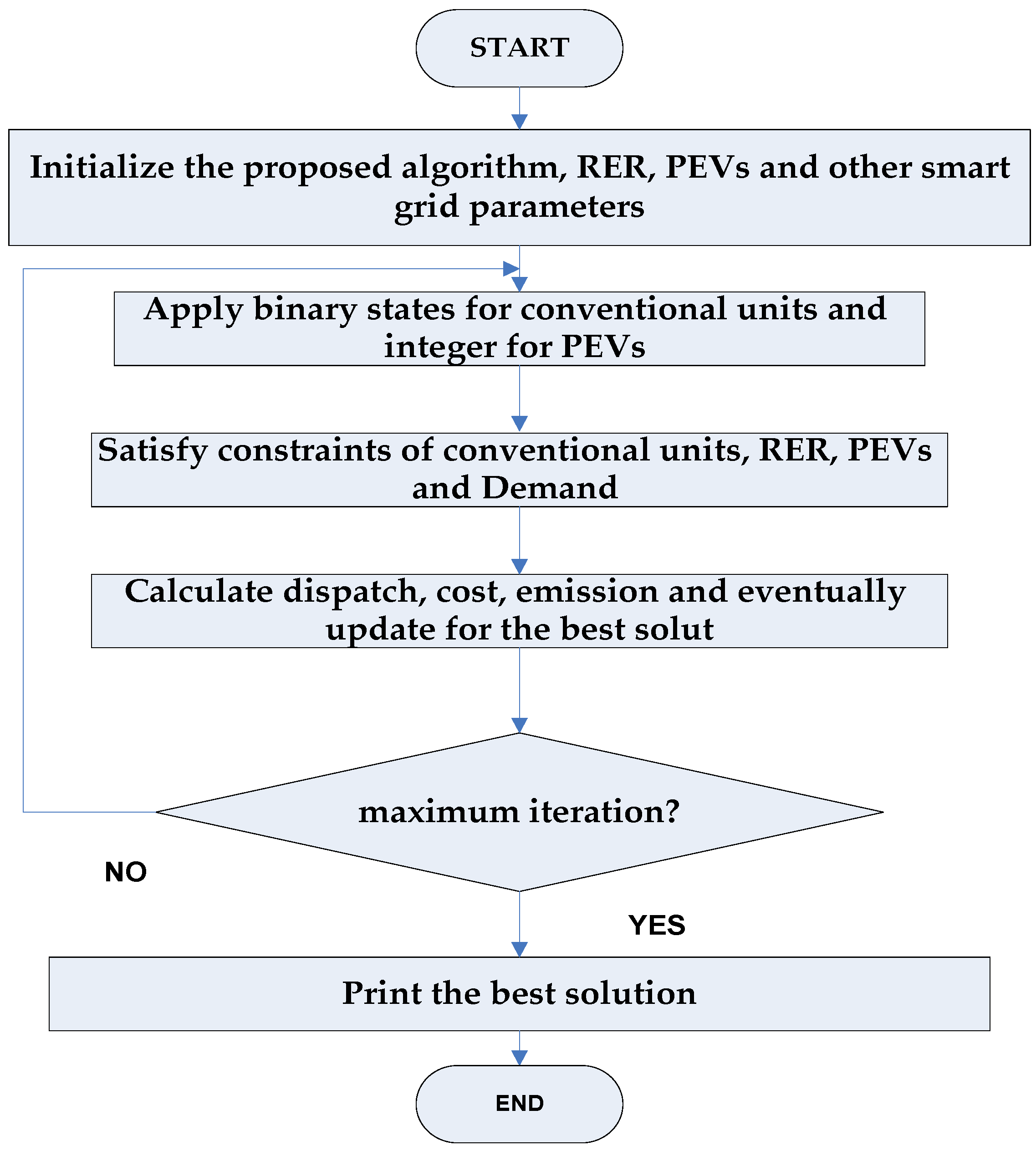
3. Unit Commitment Techniques
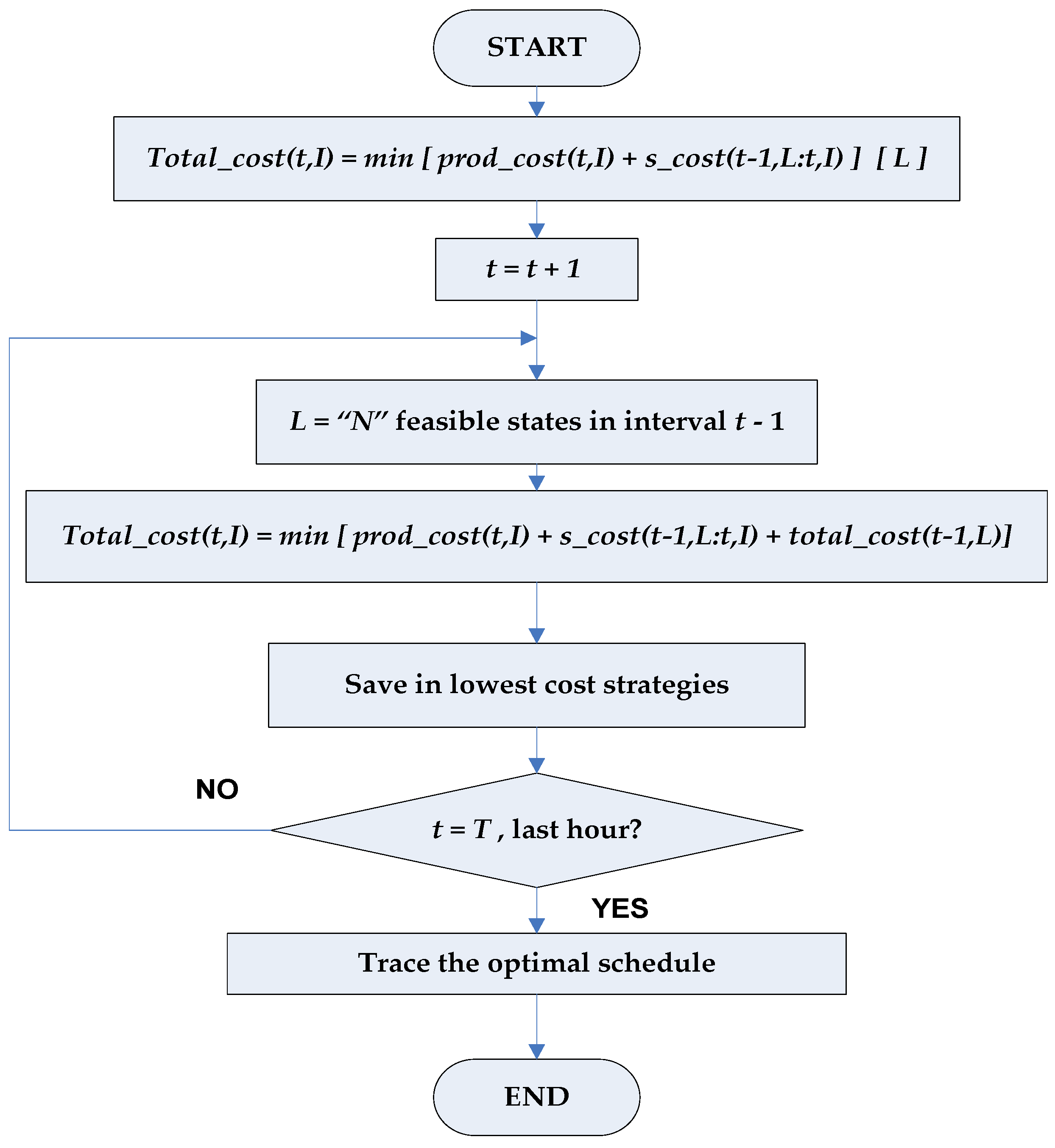
3.1. Unit Commitment Solution Dynamic Programming Technique Based
Step by Step Transition for Forward Dynamic Programming
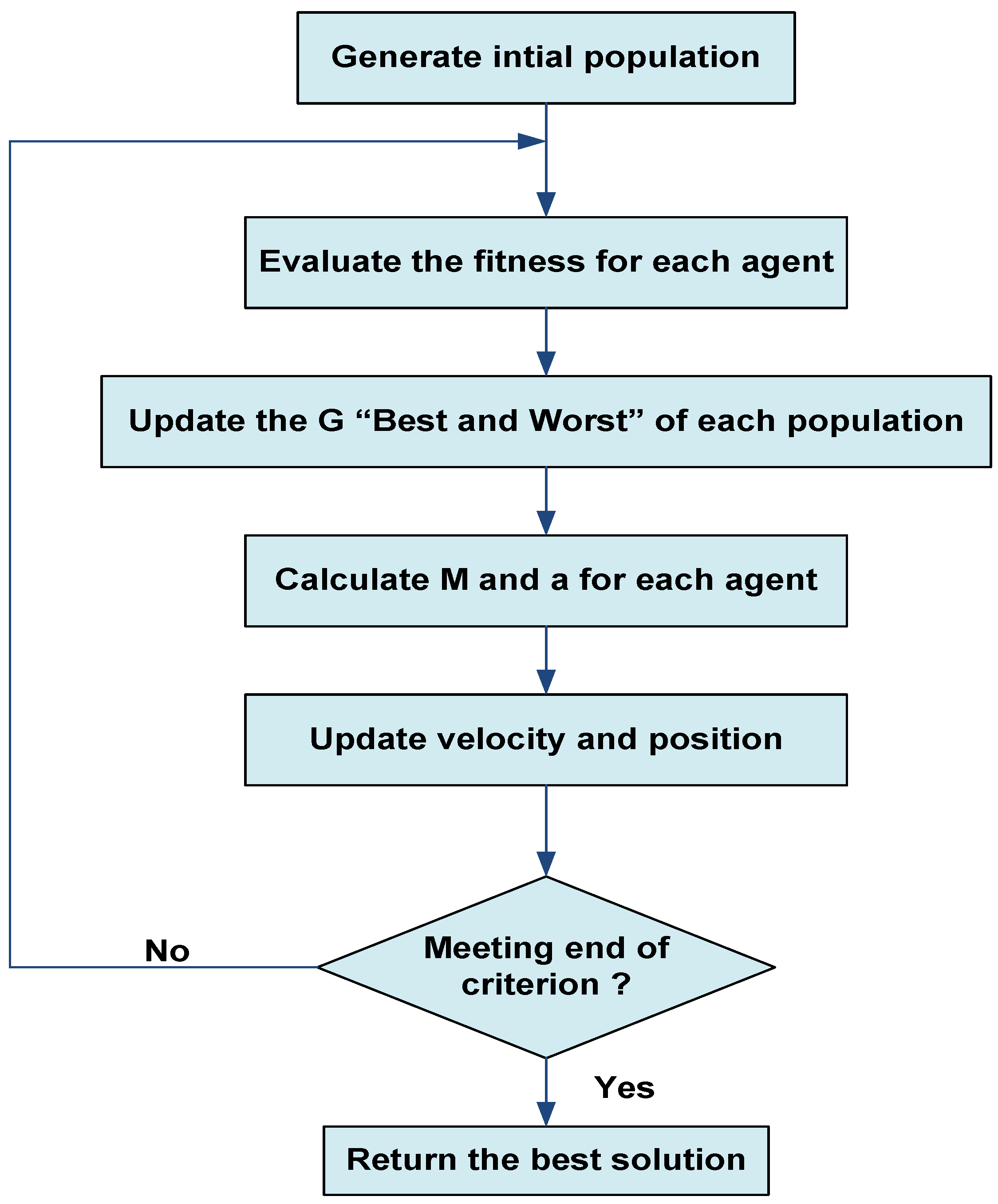
3.2. The Gravitational Search Algorithm (GSA)
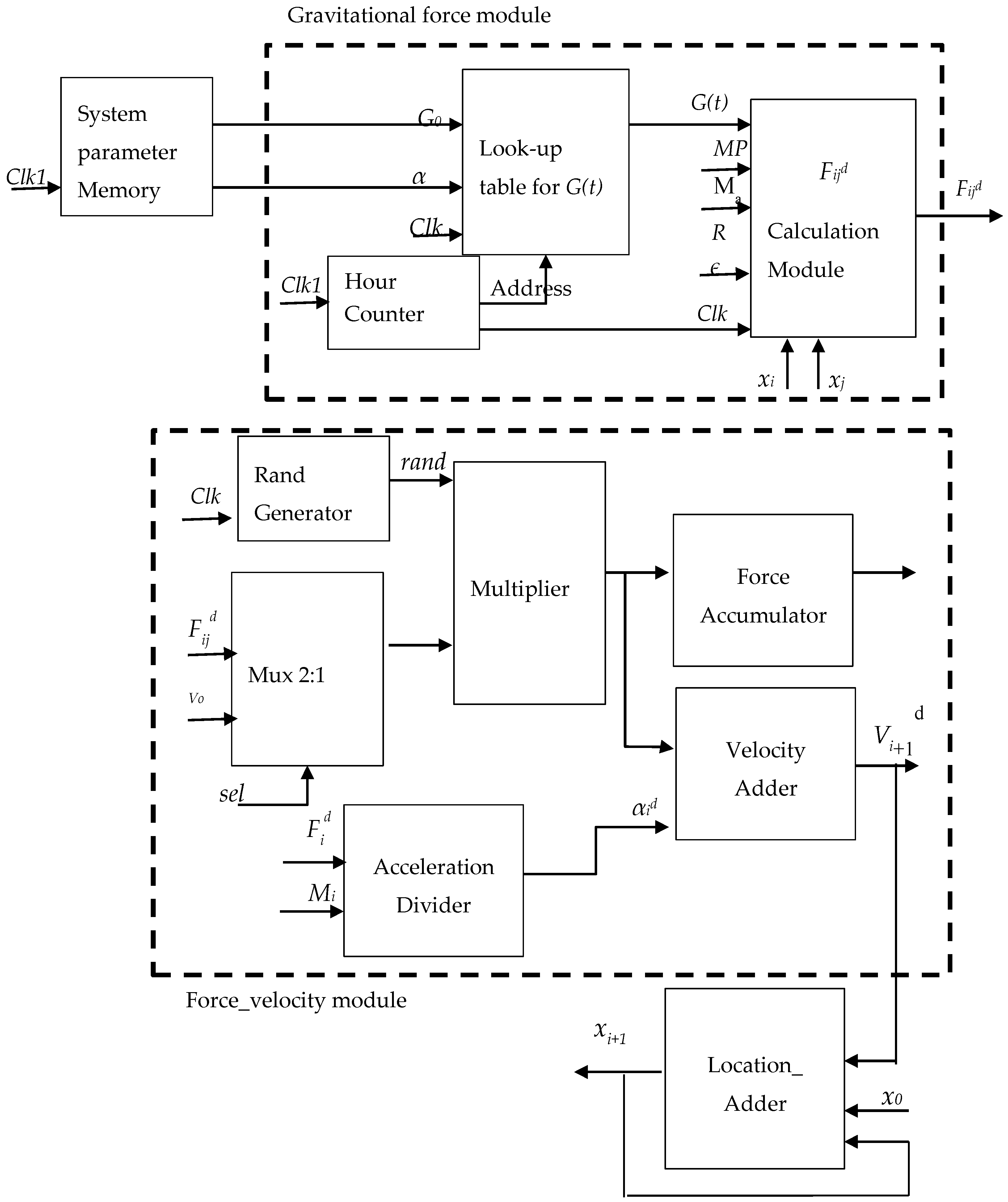
4. Hardware Implementation Based on FPGA
5. System Data
6. Simulation Results
6.1. Scenario 1 (Base Case)
6.2. Scenario 2 (PEVs and the Three Coal-Fired Units)
6.3. Scenario 3 (RERs, and Three Coal-Fired Units)
6.4. Scenario 4 (RERs, PEVs, and the Three Coal-Fired Units)
- In case 1: The start-up cost, and emission is significantly increasing by 800 $/day, 866.869 ton/day.
- In case 2: The start-up cost, and emission is significantly increasing by 3000 $/day, 754.354 ton/day.
- In case 3: The start-up cost, and emission is significantly increasing by 500 $/day, 768.636 ton/day.
- In case 4: A significant reduction in the start-up cost by1800 $/day. However, the emission is significantly increasing by 829.781 ton/day.
7. Conclusions
Author Contributions
Funding
Conflicts of Interest
Nomenclature
| PGi | the output power of each thermal generator “i” at each hour |
| , | the minimum and maximum output limits of the i-th thermal generator respectively |
| the total active transmission line losses of the system at each hour | |
| the current of each feeder i at each hour in the system | |
| the transmission line resistance of each feeder in the system at each hour. | |
| the total number of feeders in the IEEE 30 bus electric system | |
| A, B, C | a quadratic fuel cost function coefficients of each thermal generator |
| NG | the conventional thermal generators’ number |
| the output power from a wind plant at each hour | |
| the output power from a solar plant at each hour | |
| A | CO2 emission factor |
| the emission penalty factor | |
| the power of each vehicle j | |
| , | the operational and maintenance cost coefficients of the batteries of PEVs. |
| the electric network’s efficiency | |
| Vehicles’ number that are linked to the network at this hour. | |
| the total vehicles in the network | |
| NG | number of conventional thermal generating units that operate at each hour in the unit commitment objective function |
| the present state of charge (SOC) | |
| the departure state of charge (SOC) | |
| the storage energy depletion at minimum level | |
| the charging up to maximum level | |
| on/off state of each unit “i” | |
| L | the states’ number to look for each interval in DP algorithm |
| N | the number of strategies to save at each step in DP algorithm |
| 2N − 1 | maximum value of X or N in DP algorithm |
References
- Lopez, C.J.; Ano, O.; Esteybar, D.O. Stochastic unit commitment & optimal allocation of reserves: A hybrid decomposition approach. IEEE Trans. Power Syst. 2018. [Google Scholar] [CrossRef]
- Elsayed, A.M.; Maklad, A.M.; Farrag, S.M. A New Priority List Unit Commitment Method for Large-Scale Power Systems. In Proceedings of the 2017 Nineteenth International Middle East Power Systems Conference (MEPCON), Cairo, Egypt, 19–21 December 2017; pp. 359–367. [Google Scholar]
- Venayagamoorthy, G.K.; Braband, G. Carbon reduction potential with intelligent control of power systems. In Proceedings of the 17th World Congress: International Federation of Automatic Control, Seoul, Korea, 6–11 July 2008. [Google Scholar]
- Nguyen, D.T.; Le, L.B. Risk-constrained profit maximization for microgrid aggregators with demand response. IEEE Trans. Smart Grid 2015, 6, 135–146. [Google Scholar] [CrossRef]
- Center for Climate and Energy Solution. Climate Solution, Technology Solution, Electrical Vehicles. Available online: www.c2es.org/content/electric-vehicles/ (accessed on 3 March 2018).
- Little, A.D.; Browning, L.; Santini, D.; Vyas, A.; Taylor, D.; Markel, T.; Duvall, M.; Graham, R.; Miller, A.; Frank, A.; et al. Comparing the Benefits and Impacts of Hybrid Electric Vehicle Options for Compact Sedan and Sport Utility Vehicles; Final Report 1006892; Electric Power Research Institute (EPRI): Palo Alto, CA, USA, 2002; Available online: http://www.evworld.com/library/EPRI_sedan_options.pdf (accessed on 13 March 2018).
- Corrigan, D.; Masias, A. Batteries for Electric and Hybrid Vehicles. In Linden’s Handbook of Batteries, 4th ed.; Reddy, T.B., Ed.; McGraw Hill: New York, NY, USA, 2011. [Google Scholar]
- Ghasemi, A.; Mortazavi, S.S.; Mashhour, E. Hourly demand response and battery energy storage for imbalance reduction of smart distribution company embedded with electric vehicles and wind farms. Renew. Energy 2016, 85, 124–136. [Google Scholar] [CrossRef]
- Morais, H.; Sousa, T.; Soares, J.; Faria, P.; Vale, Z. Distributed energy resources management using plug-in hybrid electric vehicles as a fuel-shifting demand response resource. Energy Convers. Manag. 2015, 97, 78–93. [Google Scholar] [CrossRef]
- Un-Noor, F.; Padmanaban, S.; Mihet-Popa, L.; Mollah, M.N.; Hossain, E. A Comprehensive Study of Key Electric Vehicle (EV) Components, Technologies, Challenges, Impacts, and Future Direction of Development. Energies 2017, 10, 1217. [Google Scholar] [CrossRef]
- Li, K.; Xue, Y.; Cui, S.; Niu, Q.; Yang, Z.; Luk, P. Advanced computational methods in energy, power, electric vehicles and their integration. In Proceedings of the International Conference on Life System Modeling and Simulation (LSMS2017) and International Conference on Intelligent Computing for Sustainable Energy and Environment (ICSEE 2017), Nanjing, China, 22–24 September 2017; Part III. Springer: Berlin, Germany, 1842. [Google Scholar]
- Rashed, E.; Nezamabadi-Pour, H.; Saryazd, S. GSA: A Gravitational Search Algorithm. Inf. Sci. 2009, 179, 2232–2248. [Google Scholar] [CrossRef]
- Rashedi, E.; Rashedi, E.; Nezamabadi-Pour, H. A comprehensive survey on gravitational search algorithm. Swarm Evolut. Comput. 2018, in press. [Google Scholar] [CrossRef]
- Mahdad, B.; Srairi, K. Interactive gravitational search algorithm and pattern search algorithms for practical dynamic economic dispatch. Int. Trans. Electr. Energy Syst. 2015, 25, 2289–2309. [Google Scholar] [CrossRef]
- Jiang, S.; Wang, Y.; Ji, Z. Convergence analysis and performance of an improved gravitational search algorithm. Appl. Soft Comput. 2014, 24, 363–384. [Google Scholar] [CrossRef]
- Thakur, N.; Titare, L.S. Determination of unit commitment problem using dynamic programming. Int. J. Nov. Res. Electr. Mech. Eng. 2016, 3, 24–28. [Google Scholar]
- Krishnamurthy, S.; Tzoneva, R. Comparative analyses of Min-Max and Max-Max price penalty factor approaches for multi criteria power system dispatch problem with valve point effect loading using Lagrange’s method. In Proceedings of the 2011 IEEE International Conference on Power and Energy Systems (ICPS), Chennai, India, 22–24 December 2011. [Google Scholar]
- World Bank and Ecofys. Carbon Pricing Watch 2017. 2017. Available online: https://openknowledge.worldbank.org/handle/10986/26565 (accessed on 3 March 2018).
- Brigatto, G.A.A.; Carmargo, C.C.B.; Sica, E.T. Multi-Objective Optimization of Distributed Generation Portofolio Insertion Strategies. In Proceedings of the 2010 IEEE/PES Transmission and Distribution Conference and Exposition: Latin America (T&D-LA), Sao Paulo, Brazil, 8–10 November 2010. [Google Scholar]
- Altera Corporation. Overcoming Smart Grid Equipment Design Challenges with FPGAs; Altera Corporation: San Jose, CA, USA, 2013. [Google Scholar]
- Yang, Q.; An, D.; Yu, W.; Tan, Z.; Yang, X. Towards Stochastic Optimization-Based Electric Vehicle Penetration in a Novel Archipelago Microgrid. Sensors 2016, 16, 907. [Google Scholar] [CrossRef] [PubMed]
- Vadana, D.P.; Kottayil, S.K. Autonomous Control of Smart Micro Grid in Islanding Mode. Procedia Technol. 2015, 21, 204–211. [Google Scholar] [CrossRef]
- Wang, Y.; Dinavahi, V. Real-time digital multi-function protection system on reconfigurable hardware. IET Gener. Transm. Distrib. 2016, 10, 2295–2305. [Google Scholar] [CrossRef]
- Zhang, B.; Wu, Y.; Jin, Z.; Wang, Y. A Real-Time Digital Solver for Smart Substation Based on Orders. Energies 2017, 10, 1795. [Google Scholar] [CrossRef]
- Razzaghi, R.; Mitjans, M.; Rachidi, F.; Paolone, M. An automated FPGA real-time simulator for power electronics and power systems electromagnetic transient applications. Electr. Power Syst. Res. 2016, 141, 147–156. [Google Scholar] [CrossRef]
- Dufour, C.; Cense, S.; Jalili-Marandi, V.; Bélanger, J. Review of state-of-the-art solver solutions for HIL simulation of power systems, power electronic and motor drives. In Proceedings of the 15th European Conference on Power Electronics and Applications (EPE), Lille, France, 2–6 September 2013; pp. 1–12. [Google Scholar]
- Zhang, B.; Fu, S.; Jin, Z.; Hu, R. A Novel FPGA-Based Real-Time Simulator for Micro-Grids. Energies 2017, 10, 1239. [Google Scholar] [CrossRef]
- He, D.; Tan, Z.; Harley, R.G. Chance constrained unit commitment with wind generation and superconducting magnetic energy storages. In Proceedings of the IEEE Power and Energy Society General Meeting, San Diego, CA, USA, 22–26 July 2012. [Google Scholar]
- Saber, A.Y.; Venayagamoorthy, G.K. Efficient utilization of renewable energy sources by gridable vehicles in cyber-physical energy systems. IEEE Syst. J. 2010, 4, 285–294. [Google Scholar] [CrossRef]
- International Renewable Energy Agency (IRENA). Renewable Power Generation Costs in 2017; International Renewable Energy Agency: Abu Dhabi, UAE, 2018; Available online: http://www.irena.org/publications/2018/Jan/Renewable-power-generation-costs-in-2017 (accessed on 18 March 2018).
- ElAzab, H.-A.I.; Swief, R.A.; El-Amary, N.H.; Temraz, H.K. Unit Commitment Towards Decarbonized Network Facing Fixed and Stochastic Resources Applying Water Cycle Optimization. Energies 2018, 11, 1140. [Google Scholar] [CrossRef]


| Energy Resource | CO2 Emission Factor (ton/kWh) |
|---|---|
| Wind | 21.0 × 10⁻⁶ |
| Hydro | 15.0 × 10⁻⁶ |
| Solar | 6.00 × 10⁻⁶ |
| Natural Gas | 5.99 × 10⁻⁴ |
| Fuel oil | 8.93 × 10⁻⁴ |
| Coal | 9.55 × 10⁻⁴ |
| Algorithm Parameter | Value |
|---|---|
| Number of agents | 50 |
| Maximum number of iterations (T) | 1000 |
| Go | 100 |
| α | 20 |
| Unit | Pmin (MW) | Pmax (MW) | Ramp up (MW/h) | Ramp down (MW/h) | Intial State at Time |
|---|---|---|---|---|---|
| G1 | 30 | 600 | 200 | 50 | On |
| G2 | 30 | 600 | 200 | 20 | Off |
| G3 | 20 | 400 | 200 | 50 | On |
| Unit | Fuel Consumption Function | Startup Cost ($) | Shutdown Cost ($) | ||
|---|---|---|---|---|---|
| A (MBtu) | B (MBtu/MWh) | C (MBtu/MWh2) | |||
| G1 | 176.9 | 13.5 | 0.04 | 1200 | 800 |
| G2 | 129.9 | 40.6 | 0.001 | 1000 | 500 |
| G3 | 137.4 | 17.6 | 0.005 | 1500 | 800 |
| Hour | Wind (MW) | Solar (MW) | Hour | Wind (MW) | Solar (MW) |
|---|---|---|---|---|---|
| 1 | 8.2 | 0 | 13 | 59.0 | 65.0 |
| 2 | 11.4 | 0 | 14 | 78.1 | 58.27 |
| 3 | 66.9 | 0 | 15 | 44.9 | 53.79 |
| 4 | 69.8 | 0 | 16 | 19.5 | 47.06 |
| 5 | 55.4 | 0 | 17 | 3.7 | 27.11 |
| 6 | 50.9 | 0 | 18 | 16.5 | 11 |
| 7 | 4.6 | 5 | 19 | 72.2 | 0 |
| 8 | 49.3 | 22.04 | 20 | 73.3 | 0 |
| 9 | 45.6 | 53.95 | 21 | 65.3 | 0 |
| 10 | 10.1 | 67.4 | 22 | 24.5 | 0 |
| 11 | 24.8 | 67.32 | 23 | 49.9 | 0 |
| 12 | 37.3 | 69.64 | 24 | 40.3 | 0 |
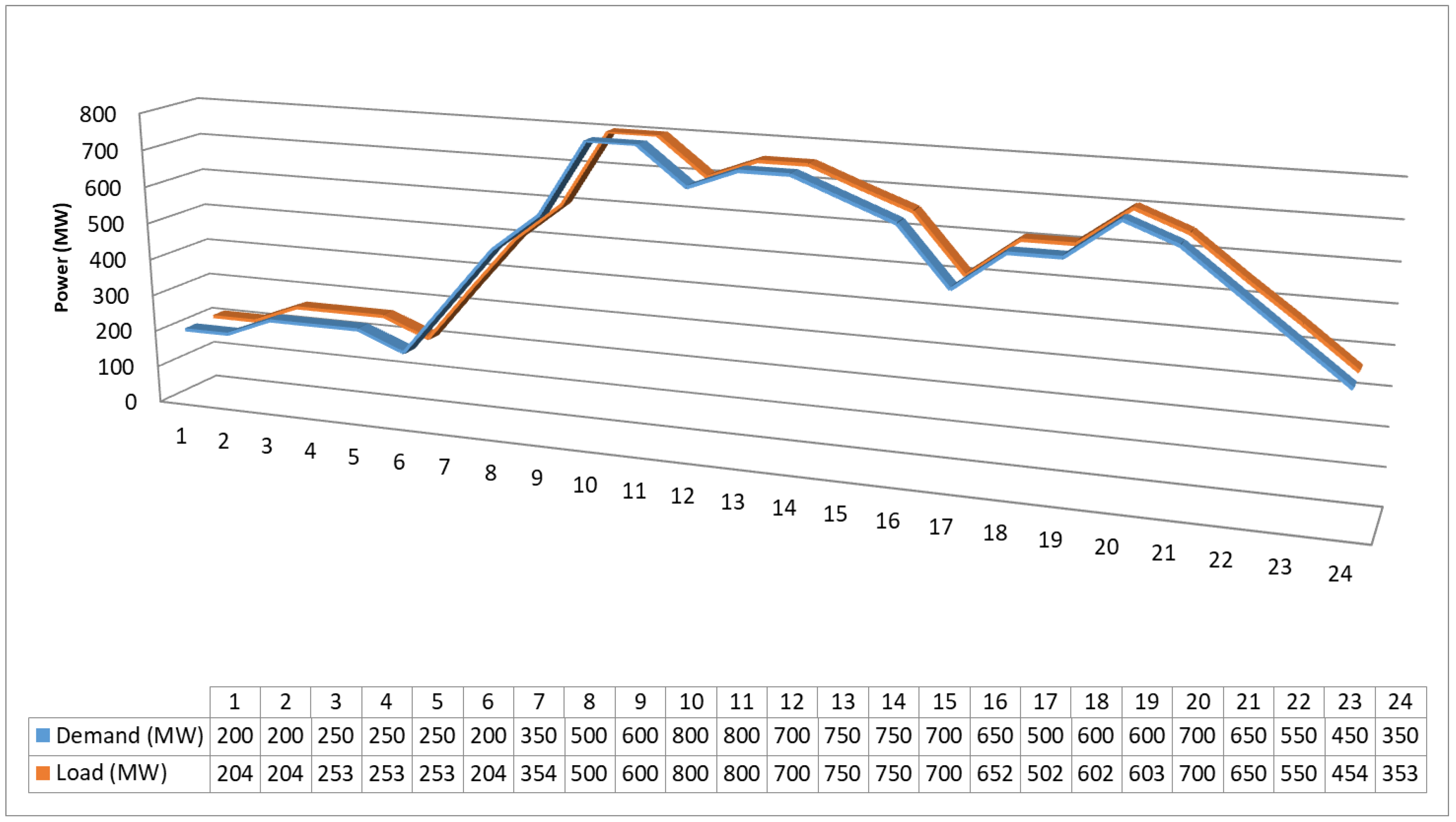
| Time (Hour) | ThermUnit-1 (MW) | ThermUnit-2 (MW) | ThermUnit-3 (MW) | Emission (ton) | Demand (MW) | Losses (MW) |
|---|---|---|---|---|---|---|
| 1 | 68.22 | 0 | 135.48 | 195 | 200 | 3.70 |
| 2 | 68.19 | 0 | 135.51 | 195 | 200 | 3.70 |
| 3 | 74.05 | 0 | 182.36 | 245 | 250 | 6.41 |
| 4 | 74.01 | 0 | 182.39 | 245 | 250 | 6.41 |
| 5 | 74.05 | 0 | 182.36 | 245 | 250 | 6.41 |
| 6 | 68.19 | 0 | 135.52 | 195 | 200 | 3.71 |
| 7 | 86.34 | 0 | 280.36 | 350 | 350 | 16.69 |
| 8 | 91.97 | 127.24 | 324.13 | 519 | 500 | 43.33 |
| 9 | 94.8 | 206.48 | 344.67 | 617 | 600 | 45.94 |
| 10 | 98.43 | 396.62 | 379.46 | 835 | 800 | 74.51 |
| 11 | 98.65 | 403.05 | 371.53 | 834 | 800 | 73.22 |
| 12 | 51.77 | 383.05 | 321.53 | 722 | 700 | 56.34 |
| 13 | 95.77 | 363.05 | 355.95 | 778 | 750 | 64.54 |
| 14 | 97.56 | 348.77 | 368.78 | 778 | 750 | 65.10 |
| 15 | 92.9 | 328.77 | 333.15 | 721 | 700 | 54.81 |
| 16 | 88.53 | 308.77 | 298.28 | 664 | 650 | 45.58 |
| 17 | 144.06 | 0 | 400 | 520 | 500 | 44.06 |
| 18 | 94.06 | 200 | 351.89 | 617 | 600 | 45.95 |
| 19 | 93.96 | 207.33 | 341.64 | 614 | 600 | 42.93 |
| 20 | 96.44 | 297.66 | 362.93 | 723 | 700 | 57.03 |
| 21 | 92.23 | 277.66 | 327.72 | 666 | 650 | 47.62 |
| 22 | 58.96 | 257.66 | 277.72 | 663 | 550 | 44.34 |
| 23 | 99.18 | 0 | 383.45 | 461 | 450 | 32.63 |
| 24 | 0 | 0 | 372.75 | 356 | 350 | 22.75 |
| Start-up cost | Emissions | |||||
| 3800.0 $/day | 12,661.12 ton/day | |||||
| Algorithm | Modes | Start-up Cost ($/day) | Emissions (ton/day) | Losses (MW/day) |
|---|---|---|---|---|
| GSA | Scenario 1 | 3800 | 12,661.119 | 907.716 |
| Scenario 2 | 7300 | 12,580.372 | 789.9 | |
| Scenario 3 | 5300 | 11,236.486 | 920.011 | |
| Scenario 4 | 5300 | 11,257.064 | 908.294 | |
| DP | Scenario 1 | 3800 | 12,661.119 | 908.003 |
| Scenario 2 | 7300 | 12,580.372 | 789.9 | |
| Scenario 3 | 5300 | 11,236.481 | 920.011 | |
| Scenario 4 | 5300 | 11,257.064 | 908.294 |
| Algorithm | Modes | Start-up Cost ($/day) | Emissions (ton/day) | Percentage of Emissions | Notes |
|---|---|---|---|---|---|
| GSA | Scenario 1 | 3000 | 11,794.250 | -- | Base case |
| Scenario 2 | 4300 | 11,826.018 | +0.26935% | Increasing | |
| Scenario 3 | 4800 | 10,467.850 | −11.24616% | Decreasing | |
| Scenario 4 | 7100 | 10,427.283 | −11.59011% | Decreasing |
© 2018 by the authors. Licensee MDPI, Basel, Switzerland. This article is an open access article distributed under the terms and conditions of the Creative Commons Attribution (CC BY) license (http://creativecommons.org/licenses/by/4.0/).
Share and Cite
ElAzab, H.-A.I.; Swief, R.A.; Issa, H.H.; El-Amary, N.H.; Balbaa, A.; Temraz, H.K. FPGA Eco Unit Commitment Based Gravitational Search Algorithm Integrating Plug-in Electric Vehicles. Energies 2018, 11, 2547. https://doi.org/10.3390/en11102547
ElAzab H-AI, Swief RA, Issa HH, El-Amary NH, Balbaa A, Temraz HK. FPGA Eco Unit Commitment Based Gravitational Search Algorithm Integrating Plug-in Electric Vehicles. Energies. 2018; 11(10):2547. https://doi.org/10.3390/en11102547
Chicago/Turabian StyleElAzab, Heba-Allah I., R. A. Swief, Hanady H. Issa, Noha H. El-Amary, Alsnosy Balbaa, and H. K. Temraz. 2018. "FPGA Eco Unit Commitment Based Gravitational Search Algorithm Integrating Plug-in Electric Vehicles" Energies 11, no. 10: 2547. https://doi.org/10.3390/en11102547
APA StyleElAzab, H.-A. I., Swief, R. A., Issa, H. H., El-Amary, N. H., Balbaa, A., & Temraz, H. K. (2018). FPGA Eco Unit Commitment Based Gravitational Search Algorithm Integrating Plug-in Electric Vehicles. Energies, 11(10), 2547. https://doi.org/10.3390/en11102547