Estimation of the Relative Arrival Time of Microseismic Events Based on Phase-Only Correlation


Abstract
1. Introduction
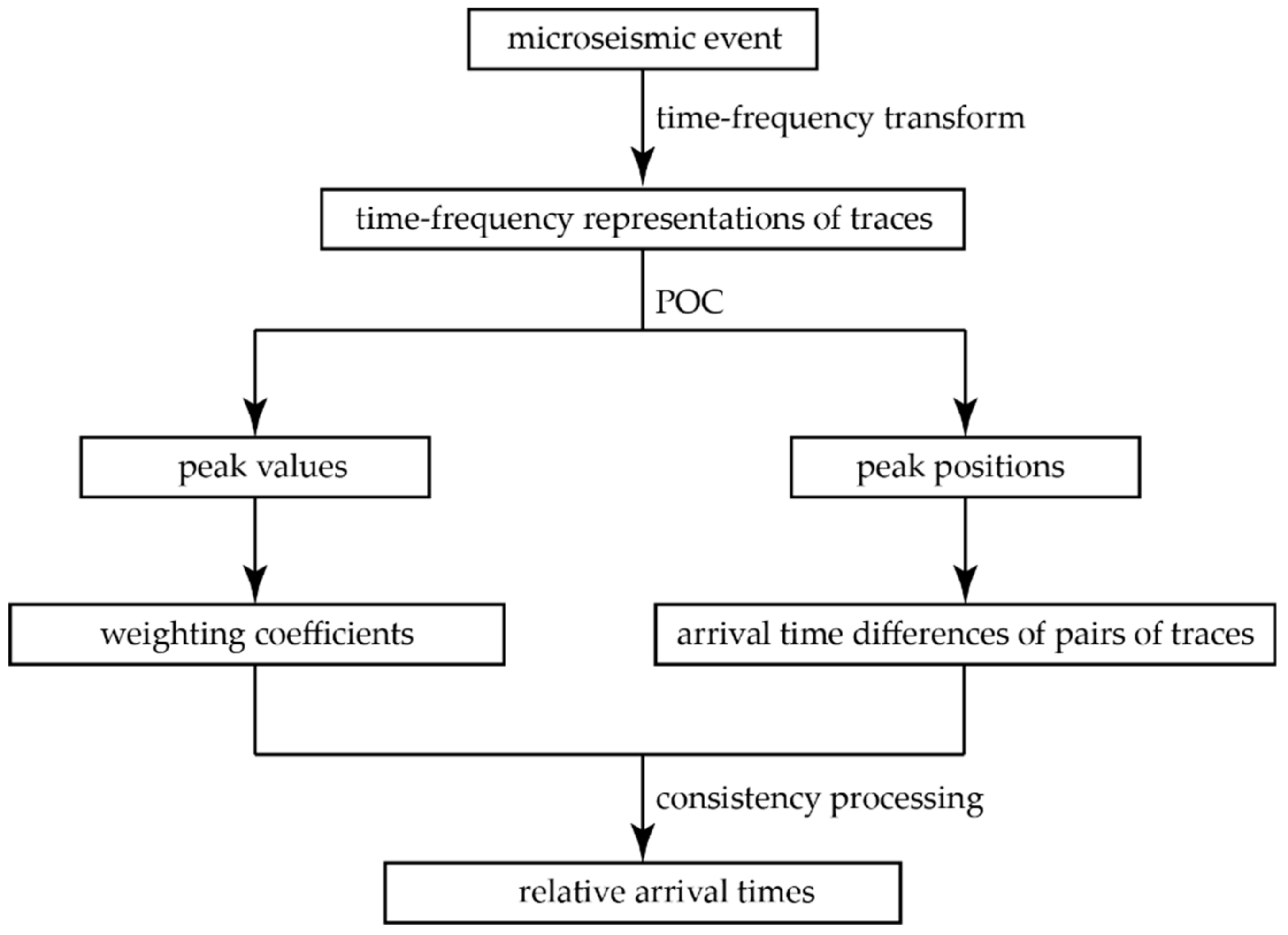
2. Methodology
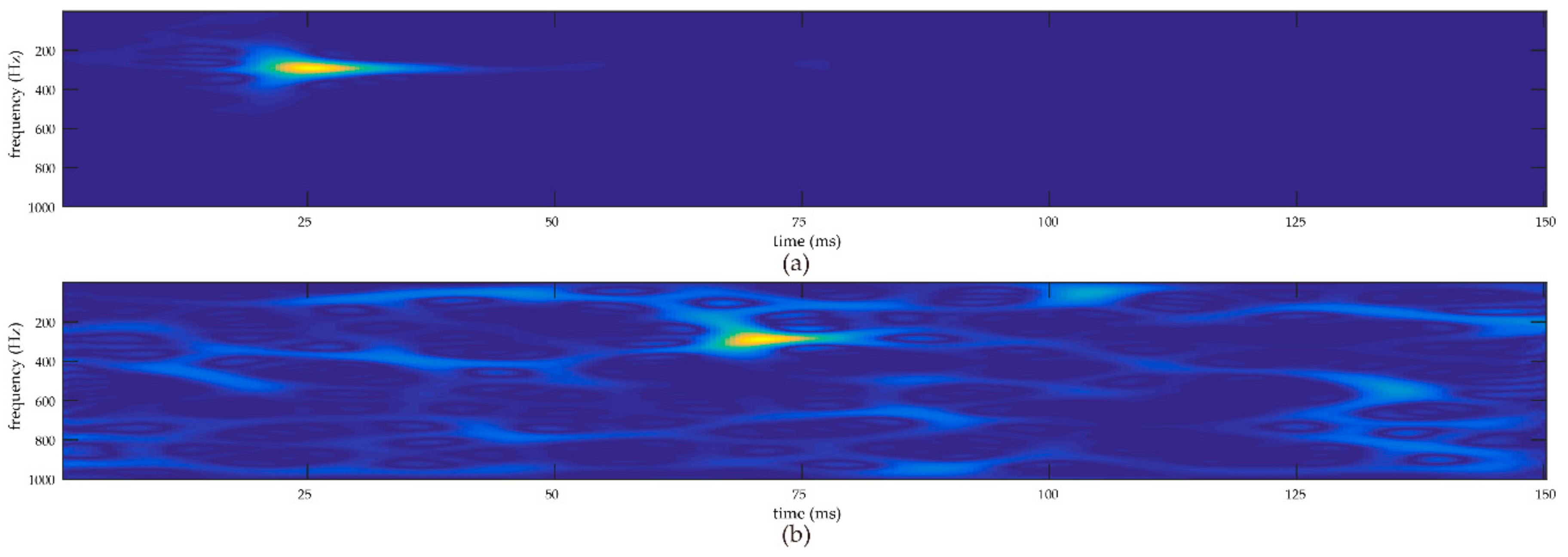
2.1. Time-Frequency Transform
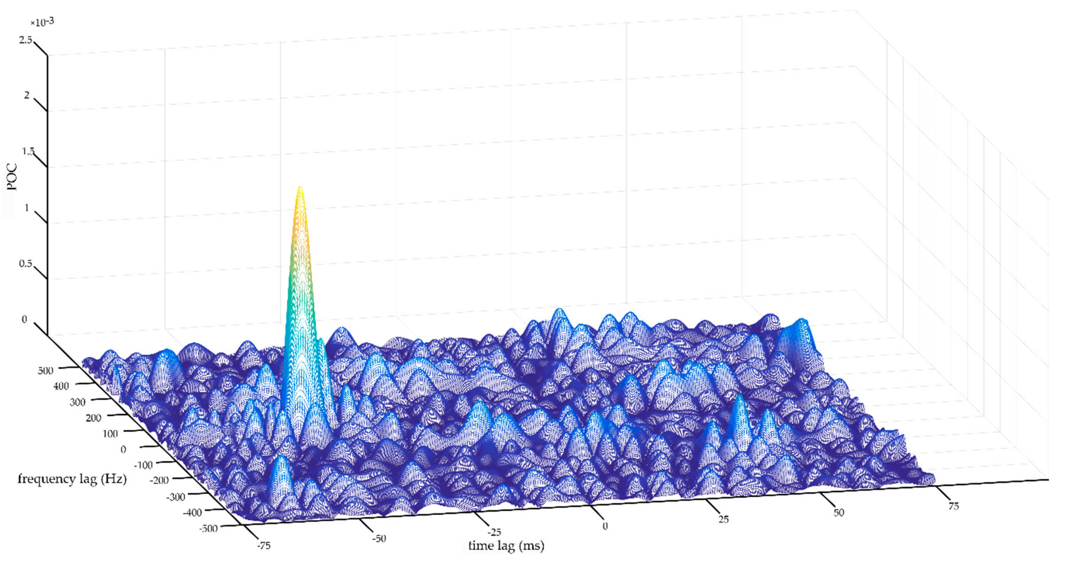
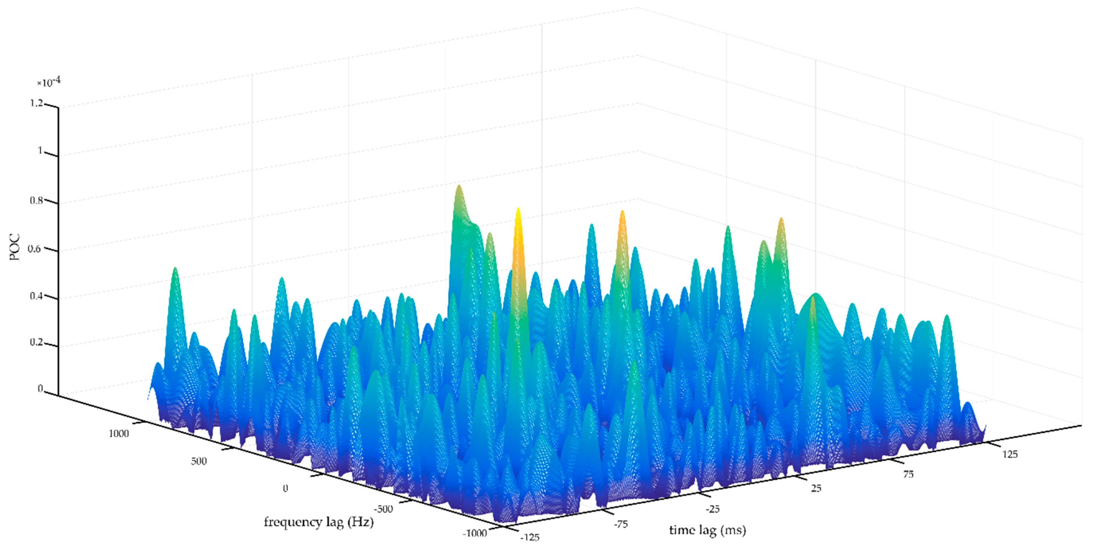
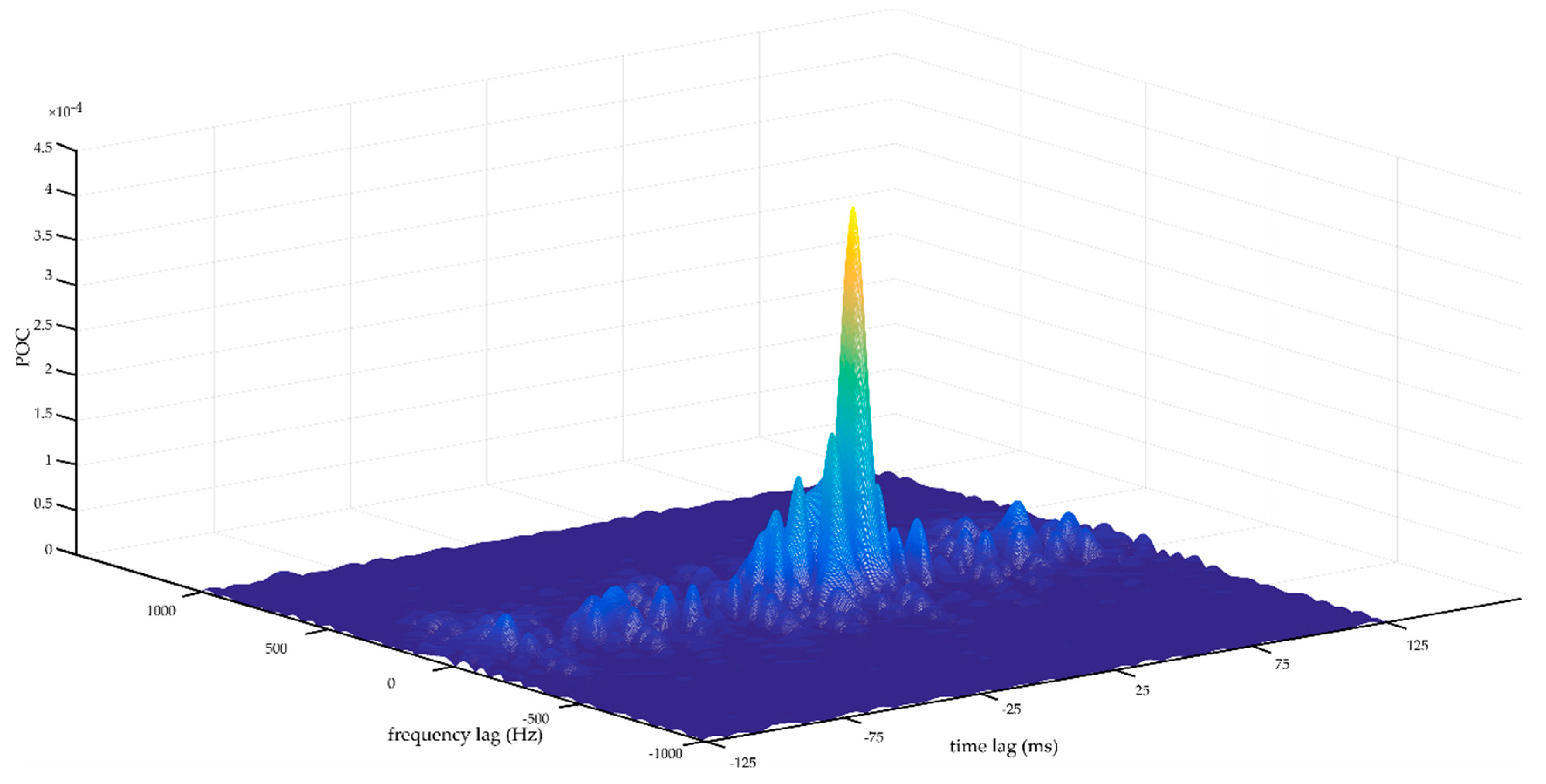
2.2. Phase-Only Correlation
2.3. Consistency Processing
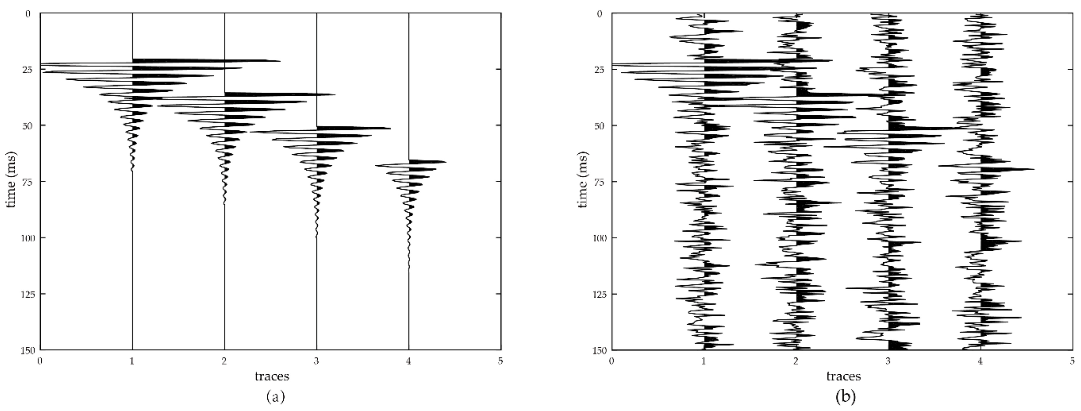
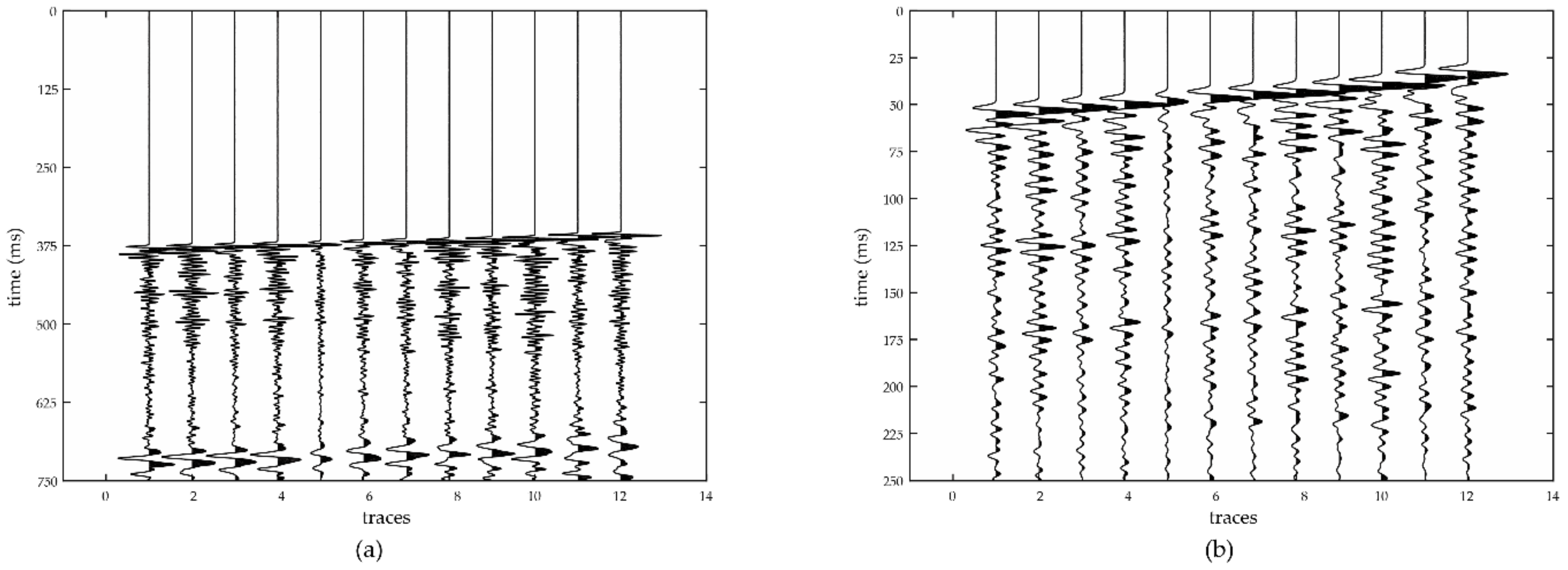
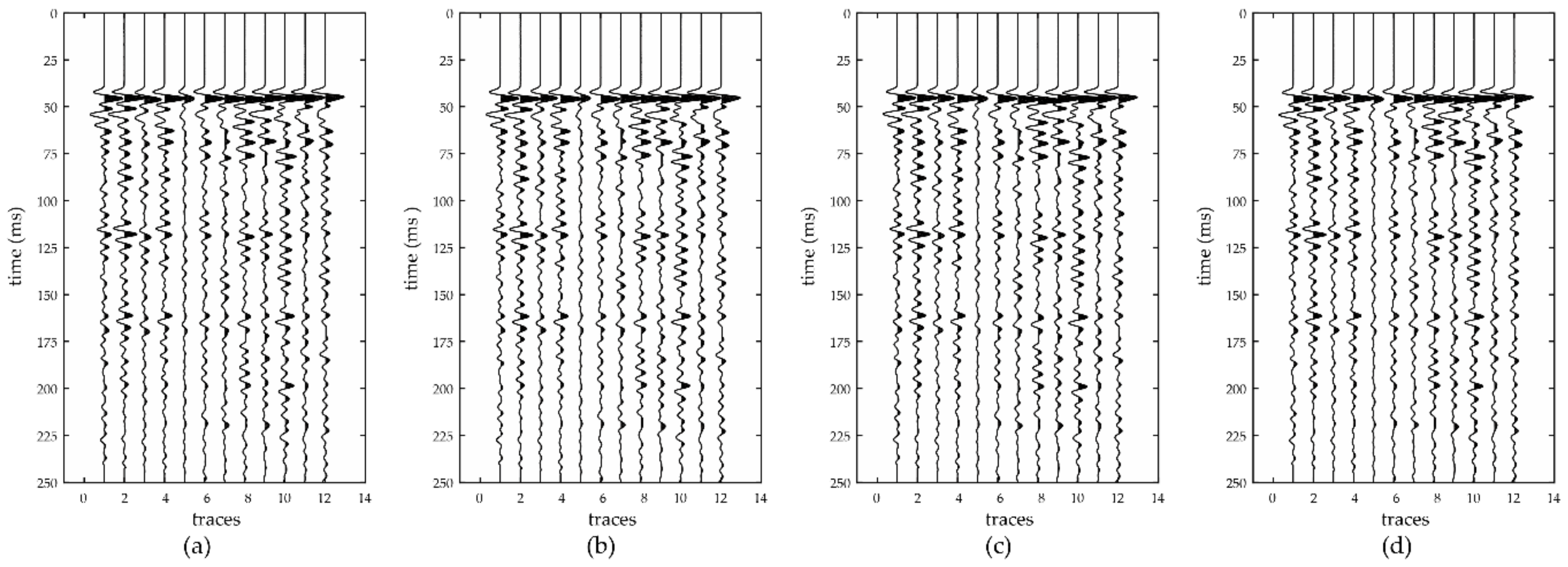
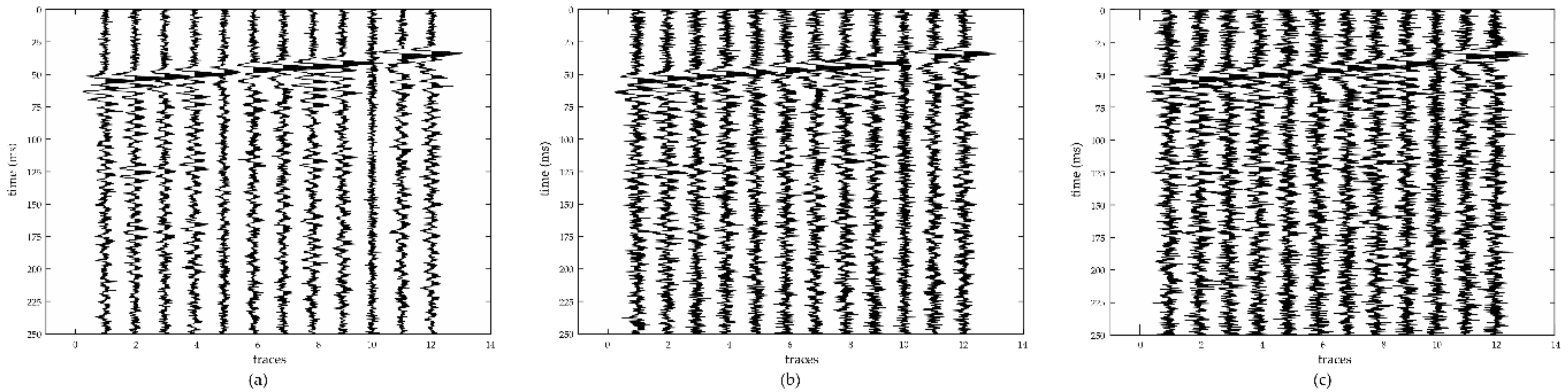
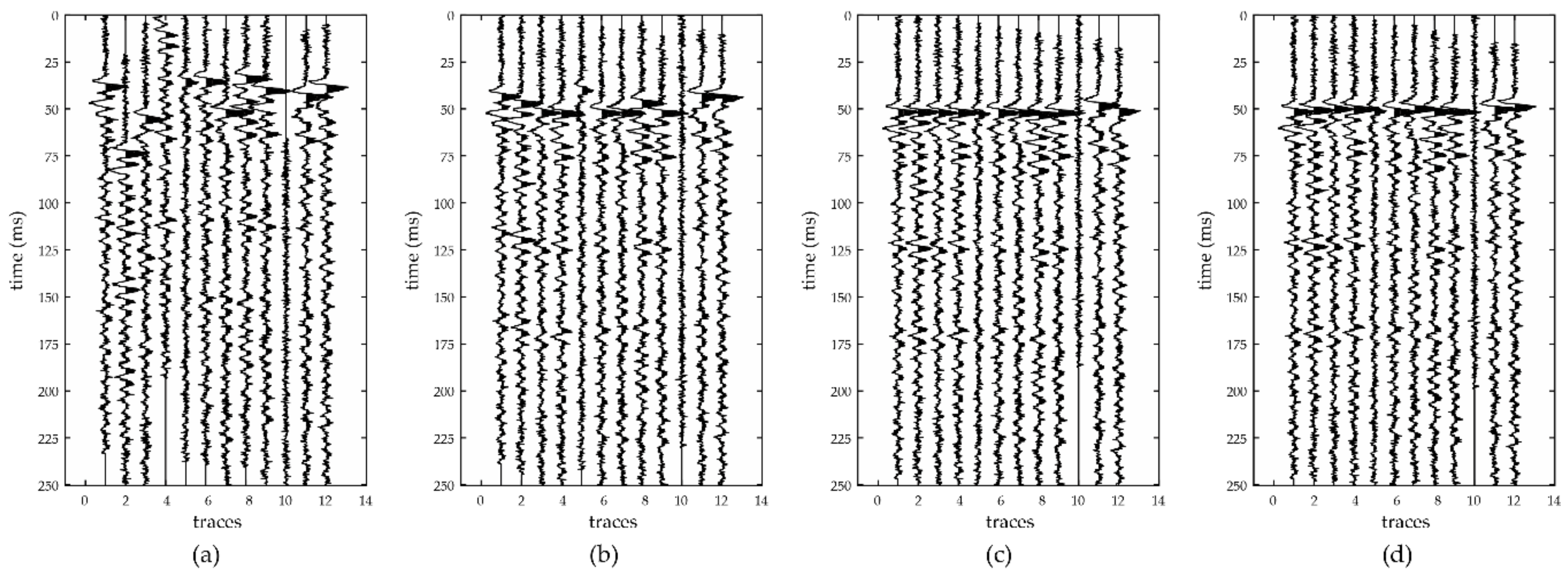
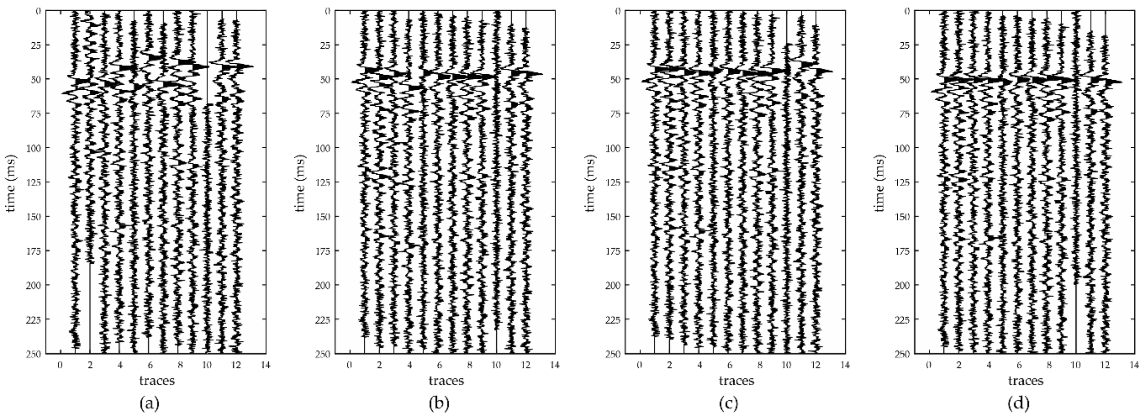
3. Synthetic Data Analysis
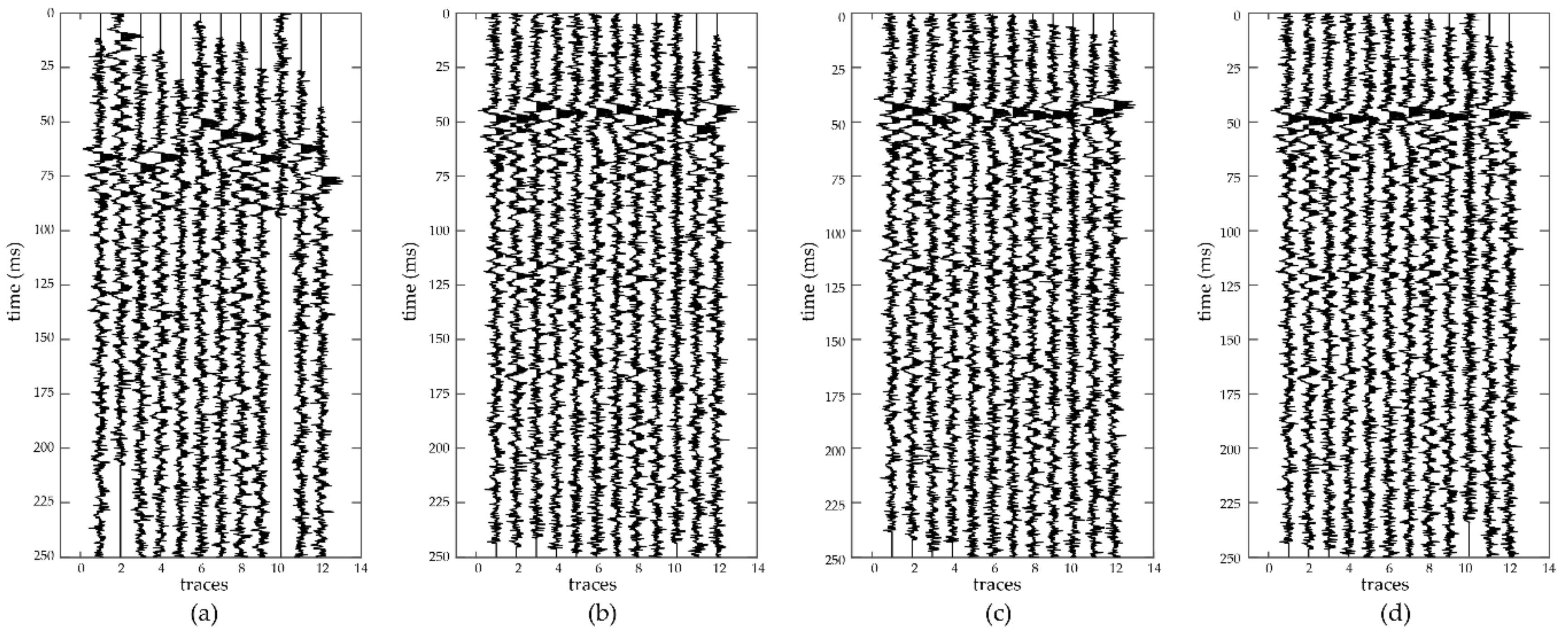
4. Field Data Analysis
5. Discussion and Conclusions
Author Contributions
Funding
Conflicts of Interest
References
- Fujii, Y.; Ishijima, Y.; Deguchi, G. Prediction of coal face rockbursts and microseismicity in deep longwall coal mining. Int. J. Rock Mech. Min. Sci. 1997, 34, 85–96. [Google Scholar] [CrossRef]
- Ge, M. Efficient mine microseismic monitoring. Int. J. Coal Geol. 2005, 64, 44–56. [Google Scholar] [CrossRef]
- Daniels, J.; Waters, G.; Le Calvez, J.; Bentley, D.; Lassek, J. Contacting More of the Barnett Shale through an Integration of Real-Time Microseismic Monitoring, Petrophysics, and Hydraulic Fracture Design. In Proceedings of the SPE Annual Technical Conference and Exhibition, Anaheim, CA, USA, 11–14 November 2007. [Google Scholar] [CrossRef]
- Maxwell, S.C.; Rutledge, J.; Jones, R.; Fehler, M. Petroleum reservoir characterization using downhole microseismic monitoring. Geophysics 2010, 75, 129–137. [Google Scholar] [CrossRef]
- Tenma, N.; Yamaguchi, T.; Zyvoloski, G. The Hijiori hot dry rock test site, Japan: Evaluation and optimization of heat extraction from a two-layered reservoir. Geothermics 2008, 37, 19–52. [Google Scholar] [CrossRef]
- Verdon, J.P.; Kendall, J.M.; White, D.J.; Angus, D.A. Linking microseismic event observations with geomechanical models to minimise the risks of storing CO2 in geological formations. Earth Planet. Sci. Lett. 2011, 305, 143–152. [Google Scholar] [CrossRef]
- Wilson, M.P.; Worrall, F.; Davies, R.J.; Almond, S. Fracking: How far from faults? Geomech. Geophys. Geo-Energy Geo-Resour. 2018, 4, 193–199. [Google Scholar] [CrossRef]
- Dyskin, A.V.; Basarir, H.; Doherty, J.; Elchalakani, M.; Joldes, G.R.; Karrech, A.; Lehane, B.; Miller, K. Computational monitoring in real time: Review of methods and applications. Geomech. Geophys. Geo-Energy Geo-Resour. 2018, 4, 235–271. [Google Scholar] [CrossRef]
- Ge, M.; Kaiser, P.K. Interpretation of physical status of arrival picks for microseismic source location. Bull. Seismol. Soc. Am. 1990, 80, 1643–1660. [Google Scholar]
- Rutledge, J.T.; Phillips, W.S. Hydraulic stimulation of natural fractures as revealed by induced microearthquakes, Carthage Cotton Valley gas field, east Texas. Geophysics 2003, 68, 441–452. [Google Scholar] [CrossRef]
- Reyes-Montes, J.M.; Pettitt, W.; Hemmings, B.; Young, R.P. Application of Relative Location Techniques to Induced Microseismicity from Hydraulic Fracturing. In Proceedings of the SPE Annual Technical Conference and Exhibition, Society of Petroleum Engineers, New Orleans, LA, USA, 4–7 October 2009. [Google Scholar] [CrossRef]
- Dong, L.; Li, X. A microseismic/acoustic emission source location method using arrival times of PS waves for unknown velocity system. Int. J. Distrib. Sens. Netw. 2013, 9, 307489. [Google Scholar] [CrossRef]
- Akram, J.; Eaton, D.W. A review and appraisal of arrival-time picking methods for downhole microseismic data. Geophysics 2016, 81, KS71–KS91. [Google Scholar] [CrossRef]
- García, L.; Álvarez, I.; Benítez, C.; Titos, M.; Bueno, Á.; Mota, S.; de la Torre, Á.; Segura, J.C.; Alguacil, G.; Díaz-Moreno, A.; et al. Advances on the automatic estimation of the P. wave onset time. Ann. Geophys. 2016, 59, S0434. [Google Scholar] [CrossRef]
- Allen, R.V. Automatic earthquake recognition and timing from single traces. Bull. Seismol. Soc. Am. 1978, 68, 1521–1532. [Google Scholar]
- Zhang, R.; Zhang, L. Method for identifying micro-seismic P-arrival by time-frequency analysis using intrinsic time-scale decomposition. Acta Geophys. 2015, 63, 468–485. [Google Scholar] [CrossRef]
- Chen, Z.; Stewart, R. A multi-window algorithm for real-time automatic detection and picking of P-phases of microseismic events. In Proceedings of the SEG Houston 2005 Annual Meeting, Houston, TX, USA, 6–11 November 2005; pp. 1288–1291. [Google Scholar] [CrossRef]
- Chen, Z.; Stewart, R. Multi-window algorithm for detecting seismic first arrivals. In Proceedings of the CSEG National Convention, Calgary, AB, Canada, 18 May 2005; pp. 355–358. [Google Scholar]
- Song, F.; Kuleli, H.S.; Toksöz, M.N.; Ay, E.; Zhang, H. An improved method for hydrofracture-induced microseismic event detection and phase picking. Geophysics 2010, 75, A47–A52. [Google Scholar] [CrossRef]
- Withers, M.; Aster, R.; Young, C.; Beiriger, J.; Harris, M.; Moore, S.; Trujillo, J. A comparison of select trigger algorithms for automated global seismic phase and event detection. Bull. Seismol. Soc. Am. 1998, 88, 95–106. [Google Scholar] [CrossRef]
- Lee, M.; Byun, J.; Kim, D.; Choi, J.; Kim, M. Improved modified energy ratio method using a multi-window approach for accurate arrival picking. J. Appl. Geophys. 2017, 139, 117–130. [Google Scholar] [CrossRef]
- Sedlak, P.; Hirose, Y.; Enoki, M.; Sikula, J. Arrival time detection in thin multilayer plates on the basis of the Akaike information criterion. J. Acoust. Emiss. 2008, 26, 182–188. [Google Scholar]
- St-Onge, A. Akaike information criterion applied to detecting first arrival times on microseismic data. In Proceedings of the SEG Annual Meeting, Society of Exploration Geophysicists, San Antonio, TX, USA, 18–23 September 2011. [Google Scholar] [CrossRef]
- Tselentis, G.A.; Martakis, N.; Paraskevopoulos, P.; Lois, A.; Sokos, E. Strategy for automated analysis of passive microseismic data based on S.-transform, Otsu’s thresholding, and higher order statistics. Geophysics 2012, 77, KS43–KS54. [Google Scholar] [CrossRef]
- Bogiatzis, P.; Ishii, M. Continuous wavelet decomposition algorithms for automatic detection of compressional and shear-wave arrival times. Bull. Seismol. Soc. Am. 2015, 105, 1628–1641. [Google Scholar] [CrossRef]
- Mousavi, S.M.; Langston, C.A.; Horton, S.P. Automatic microseismic denoising and onset detection using the synchrosqueezed continuous wavelet transform. Geophysics 2016, 81, V341–V355. [Google Scholar] [CrossRef]
- Shang, X.; Li, X.; Morales-Esteban, A.; Dong, L. Enhancing micro-seismic P-phase arrival picking: EMD-cosine function-based denoising with an application to the AIC picker. J. Appl. Geophys. 2018, 150, 325–337. [Google Scholar] [CrossRef]
- Moriya, H.; Niitsuma, H. Precise detection of a P-wave in low S/N signal by using time-frequency representations of a triaxial hodogram. Geophysics 1996, 61, 1453–1466. [Google Scholar] [CrossRef]
- Murat, M.E.; Rudman, A.J. Automated first arrival picking: A neural network approach. Geophys. Prospect. 1992, 40, 587–604. [Google Scholar] [CrossRef]
- Gou, X.; Li, Z.; Qin, N.; Jin, W. Adaptive picking of microseismic event arrival using a power spectrum envelope. Comput. Geosci. 2011, 37, 158–164. [Google Scholar] [CrossRef]
- Mousa, W.A.; Al-Shuhail, A.A.; Al-Lehyani, A. A new technique for first-arrival picking of refracted seismic data based on digital image segmentation. Geophysics 2011, 76, V79–V89. [Google Scholar] [CrossRef]
- Chen, Y. Automatic microseismic event picking via unsupervised machine learning. Geophys. J. Int. 2017, 212, 88–102. [Google Scholar] [CrossRef]
- Ross, Z.E.; Meier, M.A.; Hauksson, E. P-wave arrival picking and first-motion polarity determination with deep learning. J. Geophys. Res. Solid Earth 2018, 123, 5120–5129. [Google Scholar] [CrossRef]
- Zhang, H.; Thurber, C.; Rowe, C. Automatic p-wave arrival detection and picking with multiscale wavelet analysis for single-component recordings. Bull. Seismol. Soc. Am. 2003, 93, 1904–1912. [Google Scholar] [CrossRef]
- Saragiotis, C.; Alkhalifah, T.; Fomel, S. Automatic traveltime picking using local time-frequency maps. Geophysics 2013, 78, T53–T58. [Google Scholar] [CrossRef]
- Akram, J.; Eaton, D.; Onge, A.S. Automatic event-detection and time-picking algorithms for downhole microseismic data processing. In Proceedings of the EAGE Passive Seismic Workshop, Amsterdam, The Netherlands, 17–20 March 2013. [Google Scholar] [CrossRef]
- Li, X.; Shang, X.; Morales-Esteban, A.; Wang, Z. Identifying P phase arrival of weak events: The Akaike Information Criterion picking application based on the Empirical Mode Decomposition. Comput. Geosci. 2017, 100, 57–66. [Google Scholar] [CrossRef]
- Zimmer, U. Microseismic design studies. Geophysics 2011, 76, WC17–WC25. [Google Scholar] [CrossRef]
- Tan, Y.; He, C. Improved methods for detection and arrival picking of microseismic events with low signal-to-noise ratios. Geophysics 2016, 81, KS93–KS111. [Google Scholar] [CrossRef]
- VanDecar, J.C.; Crosson, R.S. Determination of teleseismic relative phase arrival times using multi-channel cross-correlation and least squares. Bull. Seismol. Soc. Am. 1990, 80, 150–169. [Google Scholar]
- Eisner, L.; Abbott, D.; Barker, W.B.; Lakings, J.; Thornton, M.P.; Microseismic Inc. Noise suppression for detection and location of microseismic events using a matched filter. In Proceedings of the SEG Annual Meeting. Society of Exploration Geophysicists, Las Vegas, NV, USA, 9–14 November 2008. [Google Scholar] [CrossRef]
- Kummerow, J. Using the value of the crosscorrelation coefficient to locate microseismic events. Geophysics 2010, 75, MA47–MA52. [Google Scholar] [CrossRef]
- Ito, K.; Nakajima, H.; Kobayashi, K.; Aoki, T.; Higuchi, T. A fingerprint matching algorithm using phase-only correlation. IEICE Trans. Fundam. Electron. Commun. Comput. Sci. 2004, 87, 682–691. [Google Scholar]
- Moriya, H. Phase-only correlation of time-varying spectral representations of microseismic data for identification of similar seismic events. Geophysics 2011, 76, WC37–WC45. [Google Scholar] [CrossRef]
- Wang, S.L.; Fang, Y.; Fang, J. Diagnostic prediction of complex diseases using phase-only correlation based on virtual sample template. BMC Bioinform. 2013, 14, S11. [Google Scholar] [CrossRef] [PubMed]
- Wu, S.; Wang, Y.; Zhan, Y.; Chang, X. Automatic microseismic event detection by band-limited phase-only correlation. Phys. Earth Planet. Inter. 2016, 261, 3–16. [Google Scholar] [CrossRef]
- Zhang, L.; Wang, Y.; Chang, X. Wigner distribution based phase-only correlation. J. Appl. Geophys. 2015, 123, 277–282. [Google Scholar] [CrossRef]
- Cohen, L. Generalized phase-space distribution functions. J. Math. Phys. 1966, 7, 781–786. [Google Scholar] [CrossRef]


| Symbol | Definition |
|---|---|
| the time-frequency representation of one trace | |
| the two-dimensional (2D) discrete Fourier transform of | |
| the cross-phase spectrum between and | |
| the amplitude component of | |
| the phase component of | |
| the phase-only correlation (POC) function between and | |
| the peak value of the POC function | |
| the relative arrival time between the ith and jth traces |
| Trace Number | Trace 1 | Trace 2 | Trace 3 |
|---|---|---|---|
| Trace 2 | −15 ms | ||
| Trace 3 | −30 ms | −15 ms | |
| Trace 4 | −45 ms | −30.5 ms | −15 ms |
| Relative Arrival Times | Trace 1 | Trace 2 | Trace 3 | Trace 4 |
|---|---|---|---|---|
| Theoretical values | 0 | 15 ms | 30 ms | 45 ms |
| Estimated values | 0 | 15 ms | 30.1 ms | 45.4 ms |
| Error | 0 | 0 | 0.1 ms | 0.4 ms |
| Methods | 1st | 2nd | 3rd | 4th | 5th | 6th | 7th | 8th | 9th | 10th | 11th | 12th |
|---|---|---|---|---|---|---|---|---|---|---|---|---|
| AIC | 0 | −1.75 | −4 | −5 | −6.75 | −8.5 | −10.5 | −11.75 | −13.5 | −15 | −19 | −20.5 |
| Cross-correlation | 0 | −2.18 | −3.23 | −5.23 | −6.58 | −8.6 | −10.3 | −11.43 | −13.85 | −15.03 | −19.15 | −20.98 |
| POC (STFT) | 0 | −2 | −3.7 | −5.45 | −7.2 | −8.95 | −11 | −12.6 | −14.1 | −15.95 | −19.25 | −21.05 |
| POC (WVD) | 0 | −1.75 | −2.85 | −4.58 | −6.58 | −8.23 | −9.85 | −11.3 | −13.98 | −14.83 | −18.53 | −20.28 |
| Average | 0 | −1.93 | −3.45 | −5.07 | −6.78 | −8.57 | −10.41 | −11.78 | −13.86 | −15.2 | −18.98 | −20.7 |
| Trace Number | 1st | 2nd | 3rd | 4th | 5th | 6th | 7th | 8th | 9th | 10th | 11th |
|---|---|---|---|---|---|---|---|---|---|---|---|
| 2nd | 4.8 | ||||||||||
| 3rd | 5.2 | 4.5 | |||||||||
| 4th | 5.1 | 4.3 | 5.1 | ||||||||
| 5th | 4.8 | 3.6 | 5.4 | 4.9 | |||||||
| 6th | 5.1 | 4.2 | 5.5 | 5.3 | 5.6 | ||||||
| 7th | 5.0 | 3.6 | 5.6 | 5.1 | 5.6 | 5.5 | |||||
| 8th | 4.7 | 3.8 | 4.7 | 5.0 | 4.6 | 5.0 | 4.7 | ||||
| 9th | 5.3 | 5.0 | 5.1 | 4.9 | 4.7 | 5.0 | 4.7 | 4.5 | |||
| 10th | 1.1 | 1.2 | 1.1 | 1.0 | 1.0 | 1.0 | 1.1 | 1.0 | 1.1 | ||
| 11th | 4.1 | 3.0 | 4.8 | 4.8 | 5.0 | 5.0 | 4.6 | 3.5 | 4.3 | 1.0 | |
| 12th | 4.3 | 3.3 | 5.0 | 5.1 | 5.3 | 5.3 | 5.2 | 4.3 | 4.4 | 0.9 | 5.4 |
| Methods | 1st | 2nd | 3rd | 4th | 5th | 6th | 7th | 8th | 9th | 10th | 11th | 12th |
|---|---|---|---|---|---|---|---|---|---|---|---|---|
| AIC | 0 | −37.5 | −20.75 | 40 | −4.25 | −5.75 | −24.25 | −7 | −15.75 | −82.5 | −24.5 | −21.75 |
| Cross-correlation | 0 | −5.83 | −12.05 | −13.98 | −3.2 | −17.38 | −19 | −14.88 | −20.63 | 8.3 | −19.2 | −21.7 |
| POC (STFT) | 0 | −1.98 | −3.63 | −5.15 | −7.33 | −8.7 | −10.65 | −12.35 | −13.88 | 59.33 | −15.65 | −20.68 |
| POC (WVD) | 0 | −1.3 | −2.1 | −3.6 | −6.25 | −8.45 | −8.8 | −11.15 | −13.73 | 47.48 | −18.05 | −18.83 |
| Methods | 1st | 2nd | 3rd | 4th | 5th | 6th | 7th | 8th | 9th | 10th | 11th | 12th |
|---|---|---|---|---|---|---|---|---|---|---|---|---|
| AIC | 0 | 62.25 | −5.25 | 4.75 | −10.75 | 8.5 | −12.5 | 2.5 | −3.25 | −71.5 | −9 | −10.25 |
| Cross-correlation | 0 | −7.45 | −6.25 | −18.2 | −8.83 | −13.63 | −15.43 | −16.25 | −18.75 | 5.4 | −21.2 | −24.2 |
| POC (STFT) | 0 | −1.68 | −5.65 | −7.63 | −7.5 | −10.28 | −13.18 | −13.18 | −14.53 | −36.4 | −15.58 | −22.38 |
| POC (WVD) | 0 | −2.58 | −3.63 | −5.63 | −8.65 | −8.9 | −10.35 | −10.23 | −14.35 | 45.8 | −19.23 | −22.78 |
| Methods | 1st | 2nd | 3rd | 4th | 5th | 6th | 7th | 8th | 9th | 10th | 11th | 12th |
|---|---|---|---|---|---|---|---|---|---|---|---|---|
| AIC | 0 | 53.75 | −8.25 | −5 | −19.25 | 7.5 | 0.25 | −2 | −14 | 167 | −15 | −31.75 |
| Cross-correlation | 0 | −1.81 | 2.29 | −2.5 | -−4.6 | −5.6 | −5.75 | −11.67 | −10.75 | −0.33 | −24.17 | −16.6 |
| POC (STFT) | 0 | −3.66 | −9.22 | −4.7 | −11.9 | −10.84 | −12.45 | −14.73 | −16.78 | −17.96 | −21.18 | −19.68 |
| POC (WVD) | 0 | −2.63 | −2.96 | −5.08 | −7.46 | −6.88 | −7.06 | −9.11 | −12.8 | 9.48 | −16.74 | −19.47 |
| SNR | AIC | Cross-Correlation | POC (STFT) | POC (WVD) |
|---|---|---|---|---|
| Without noise | 0.22 | 0.20 | 0.25 | 0.22 |
| 5 dB | 18.64 | 4.2 | 1.03 | 0.62 |
| 0 dB | 17.97 | 3.19 | 1.66 | 0.91 |
| −2 dB | 17.75 | 7.06 | 2.01 | 1.29 |
© 2018 by the authors. Licensee MDPI, Basel, Switzerland. This article is an open access article distributed under the terms and conditions of the Creative Commons Attribution (CC BY) license (http://creativecommons.org/licenses/by/4.0/).
Share and Cite
Wang, P.; Chang, X.; Zhou, X. Estimation of the Relative Arrival Time of Microseismic Events Based on Phase-Only Correlation. Energies 2018, 11, 2527. https://doi.org/10.3390/en11102527
Wang P, Chang X, Zhou X. Estimation of the Relative Arrival Time of Microseismic Events Based on Phase-Only Correlation. Energies. 2018; 11(10):2527. https://doi.org/10.3390/en11102527
Chicago/Turabian StyleWang, Peng, Xu Chang, and Xiyan Zhou. 2018. "Estimation of the Relative Arrival Time of Microseismic Events Based on Phase-Only Correlation" Energies 11, no. 10: 2527. https://doi.org/10.3390/en11102527
APA StyleWang, P., Chang, X., & Zhou, X. (2018). Estimation of the Relative Arrival Time of Microseismic Events Based on Phase-Only Correlation. Energies, 11(10), 2527. https://doi.org/10.3390/en11102527