Impact of Optimum Allocation of Renewable Distributed Generations on Distribution Networks Based on Different Optimization Algorithms

Abstract

Integration of Renewable Distributed Generations (RDGs) such as photovoltaic (PV) systems and wind turbines (WTs) in distribution networks can be considered a brilliant and efficient solution to the growing demand for energy. This article introduces new robust and effective techniques like hybrid Particle Swarm Optimization in addition to a Gravitational Search Algorithm (PSOGSA) and Moth-Flame Optimization (MFO) that are proposed to deduce the optimum location with convenient capacity of RDGs units for minimizing system power losses and operating cost while improving voltage profile and voltage stability. This paper describes two stages. First, the Loss Sensitivity Factors (LSFs) are employed to select the most candidate buses for RDGs location. In the second stage, the PSOGSA and MFO are implemented to deduce the optimal location and capacity of RDGs from the elected buses. The proposed schemes have been applied on 33-bus and 69-bus IEEE standard radial distribution systems. To insure the suggested approaches validity, the numerical results have been compared with other techniques like Backtracking Search Optimization Algorithm (BSOA), Genetic Algorithm (GA), Particle Swarm Algorithm (PSO), Novel combined Genetic Algorithm and Particle Swarm Optimization (GA/PSO), Simulation Annealing Algorithm (SA), and Bacterial Foraging Optimization Algorithm (BFOA). The evaluated results have been confirmed the superiority with high performance of the proposed MFO technique to find the optimal solutions of RDGs units’ allocation. In this regard, the MFO is chosen to solve the problems of Egyptian Middle East distribution network as a practical case study with the optimal integration of RDGs.

1. Introduction

Nowadays, the electric energy industry has shown a renewed interest in distributed generation sources [1]. The presence of Renewable Distributed Generations (RDGs), especially in distribution systems, drives researchers’ interest in many major aspects and problems. On the one hand, depending on RDGs location and size, they can be beneficial in reducing power losses and increasing the overall efficiency of the power system, enabling the evolution towards a sustainable and smart grid [1,2,3,4,5,6,7]. Moreover, RDGs represent an excellent way to power microgrids that increase grid resilience through the local ability to deal with an emergency by operating off-grid (islanded mode) [2,3]. On the other hand, new difficulties arise related to stability, voltage control, and power quality issues, among others, which have to be addressed with novel research studies and innovative solutions [2,3]. However, in this research we focus on the most important topic that is to integrate RDGs into distribution networks, due to the fact that, an increasing demand for high quality, reliable electrical power, and increasing number of loads may lead up to increase the awareness of power quality both by customers and by utilities [4]. Therefore, RDGs units are considered as a convenient solution for these problems with optimal size and location in addition to their type. Installation of RDGs units has an enormous range of impacts that include environmental, economic, and technical benefits [5,6,7,8,9,10,11]. The economic and environmental advantages can be represented in the reduction of fuel savings, distribution and transmission costs and electricity prices beside reduction of greenhouse gases [7,8,9,10,11,12,13]. The technical benefits and merits are deduced in deferring upgrades of power system, voltage profile and voltage stability improvement, power loss reduction, reliability protection, and power quality assurance [5,8,9,10,11]. In recent years, many researches are focused on photovoltaic (PV) systems and wind turbines (WTs) as Renewable Distributed Generations (RDGs), which provide a cleaner power production [7,8,11,14,15,16]. According to that, these both types are considered in this work.

In recent years, RDGs integration and capacity problems were solved based on numerous mechanisms and techniques. Abdelaziz et al. [7] solved the RDGs allocation problem with a proper capacity by employing a modified Firefly Algorithm (FA). The minimization of power loss is employed as an objective function for the proposed scheme without violating the system practical constraints. Gupta et al. [8] implemented the Radial Basis Function Neural Network (RBFNN) based on a heuristic Particle Swarm Optimizer (PSO) to find the optimal location and capacity of RDGs. The main task of PSO is to increase the improvement of the computation convergence and attitude in the training operation of RBFNN. Reddy et al. [11] proposed his work in two stages. First, the author employed Power Loss Index (PLI) to find the most candidate buses for RDGs’ location. Then, the Whale Optimization Algorithm (WOA) is implemented to deduce the optimum capacity of RDGs in radial distribution systems. Sudabattula and Kowsalwa [12] implemented the Cuckoo Search Algorithm (CSA) to estimate optimum placement and capacity of wind based on distributed generators in the distribution system. The objective function of CSA is performed to minimize power loss of the distribution system. El-Fergany [17] presented the Backtracking Search Optimization Algorithm (BSOA) with two types of RDGs, PV and WT systems, to evaluate their optimal locations in distribution networks. The objective function of BSOA is adapted to decrease the system active power losses and improve the bus voltage profile with weighting factors. Singh [18] introduced Genetic Algorithm (GA) to calculate the optimal placement and size of multi RDGs units’ to reduce the system losses and power supply by the main grid, taking into account voltage boundaries at each bus of the system. Moradi and Abedini [19] proposed three scenarios for optimal allocation and size of multiple RDGs units’; at first, the GA, and then Particle Swarm Optimization (PSO) are applied. In the third scenario, a novel combined GA/PSO was produced. In this method, GA searched for the critical sites of RDGs and their sizes that were optimized by PSO. The three scenarios were compared together using multiple objective functions. Injeti [20] presented two stages. In the first stage, the Loss Sensitivity Factor (LSF) was satisfied for determining the optimal placement of RDGs units’ to reduce the search space of optimization algorithm, and then Simulation Annealing Algorithm (SA) was proposed for optimal sizing. Imran [21] introduced the LSF for critical locations of RDGs units’ installations. Then, a Bacterial Foraging Optimization Algorithm (BFOA) was implemented to find the optimal size of RDGs’ units.

Many researchers [7,8,11,12,17] have concentrated on decreasing the system losses by improving the voltage profile without taking into consideration the costs of losses and RDGs units’ installations and maintenance with their operation. Although some researchers [18,19,20,21] considered these costs in their accounts, they worked on improving voltage profile only, without reducing system losses and costs sufficiently.

This paper presents two stages to overcome these problems. First, the loss sensitivity factors (LSFs) are performed to elect the most appropriate candidate buses for RDGs installations. Then in the second stage, a hybrid PSOGSA algorithm and MFO are constructed to detect the optimum capacity of RDGs and their location from the selected candidate buses.

The objective of this work is constructed under multiple objective functions for optimum integration of RDGs units’ to minimize the total operational cost and system power loss, in addition to improve the voltage profile and its stability.

The Backward/Forward sweep (BFS) algorithm is used for power flow lateral radial distribution grids because it is easy to implement, fast, flexible, robust convergence, and it has high accuracy [22,23]. The proposed PSOGSA and MFO have been applied on 33-bus, and 69-bus IEEE radial distribution systems, and the results by both techniques have been compared with each other and with other techniques. Therefore, the superior technique will be chosen to solve the problem of Egyptian Middle East distribution network. The practical case study of Egyptian Middle East distribution network is investigated in details in the following Section 2.

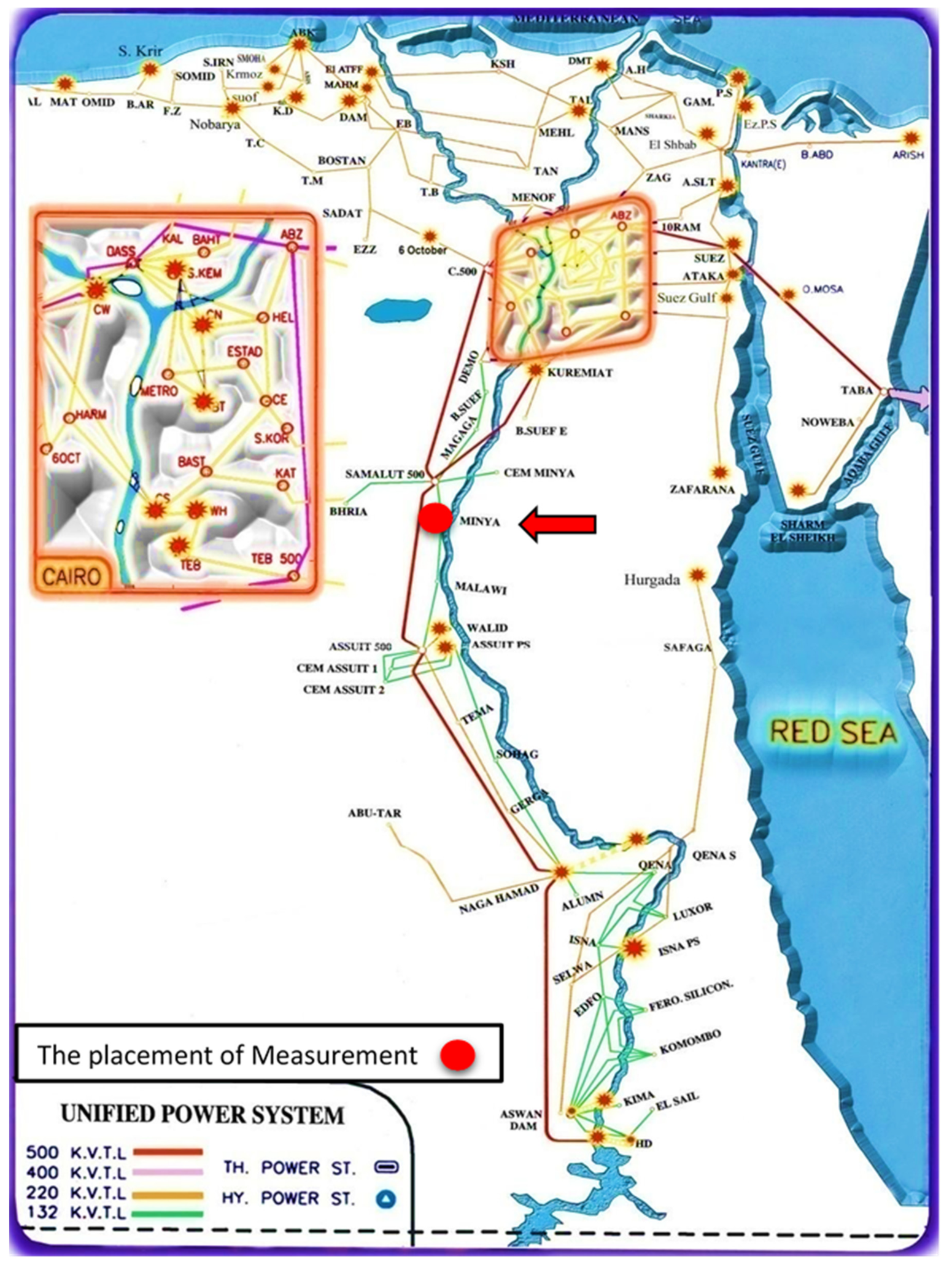
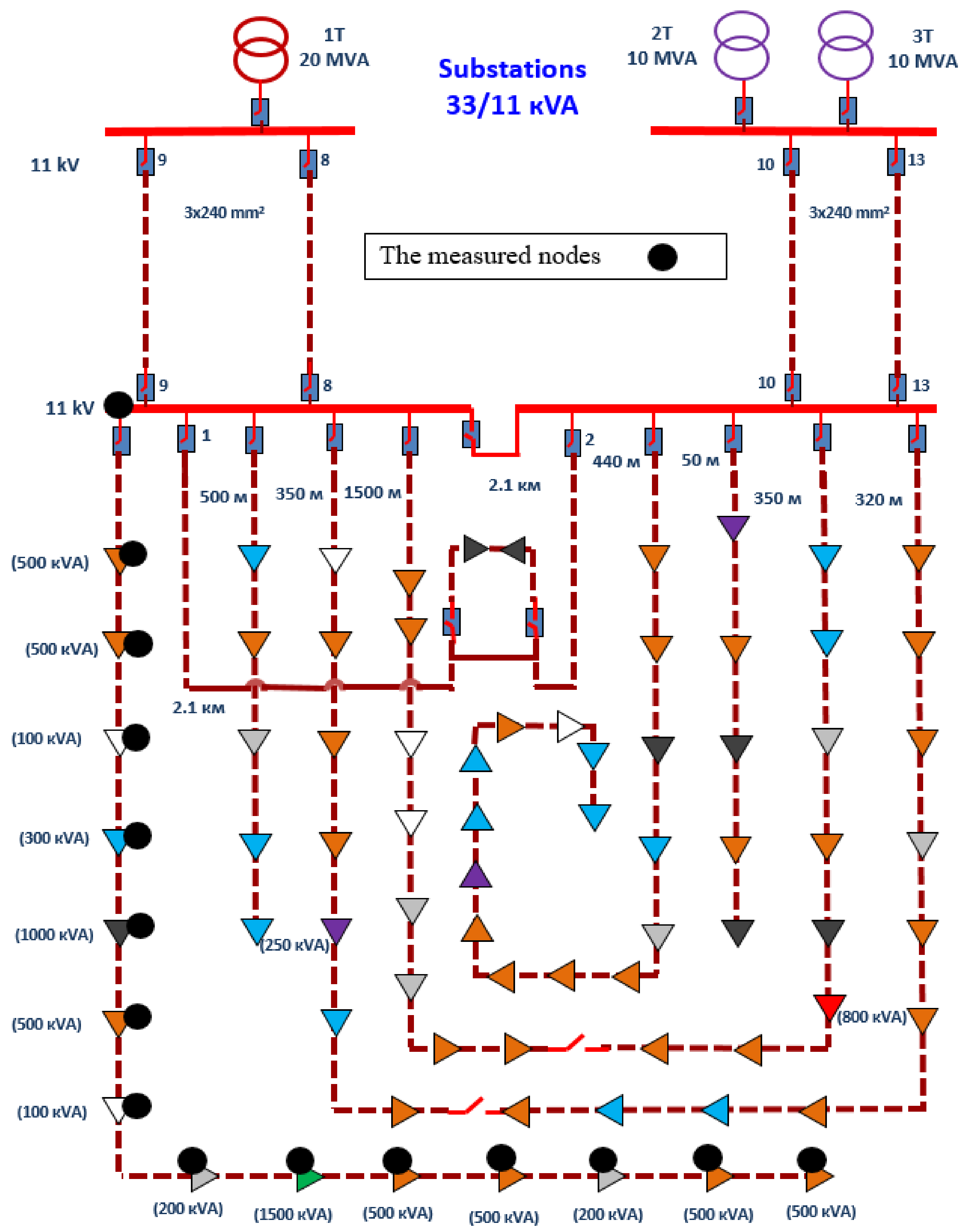
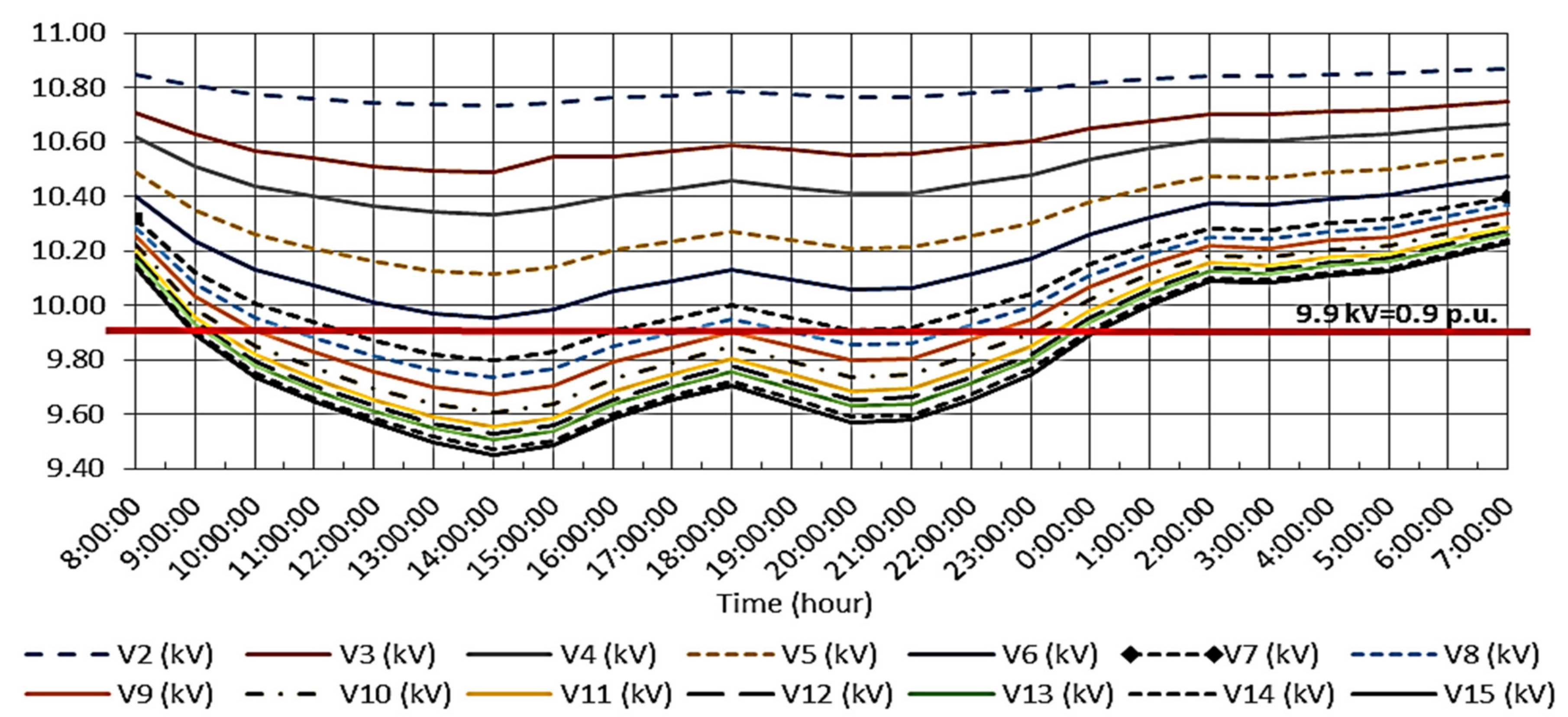
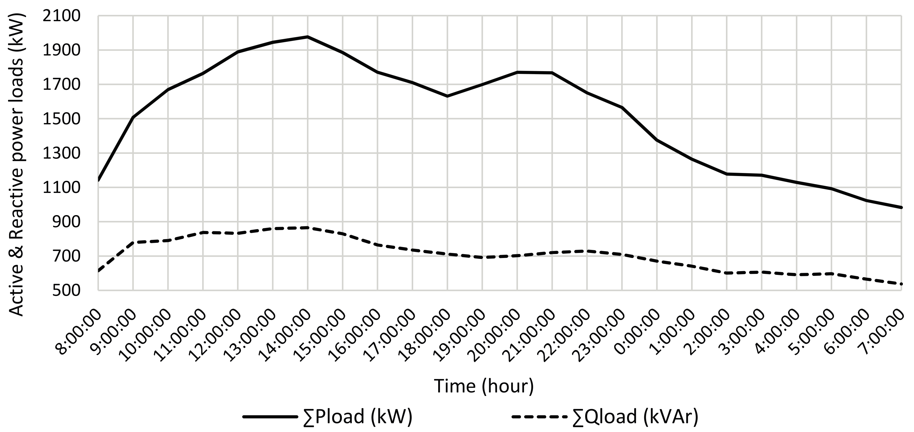
2. Investigation of the Egyptian Practical Case Study

The Middle Egypt Distribution Network (MEDN) is provided as a practical case study to analysis and deduce the power quality problems. MEDN contains important demands that suffer from voltage profile deterioration. This deterioration is considered as a noteworthy power quality problem. Moreover, measurement and analysis of voltage profile deviations and load profile within 24 h have been carried out according to IEEE Std. 1159: 2009, IEEE Std. 1346-1998 and IEC Std. [24,25,26].

Figure 1 shows the Egyptian Electrical Unified Network (EEUN) [27,28]. The EEUN in Egypt consists of six geographical regions: Cairo, Canal, Delta, Alexandria/West delta, Middle Egypt, and Upper Egypt. The transmission system of Egyptian Electricity is designed as 500 kV, 400 kV, 220 kV, 132 kV, and 66 kV levels as explained in Figure 1. In this work, we concentrated on Middle Egypt region. The electrical power system in Minya city is modeled as follows: Samalut transmission stations 500 kV, Minya transmission lines 132 kV to 33 kV, Minya distribution networks 11 kV, and the loads at 0.4 kV. The measurement and analysis have been implemented on one of Minya city distribution network 11 kV, namely, MEDN that located in the middle Egypt region as shown in Figure 1. Figure 3 illustrates the 15 bus system that is measured and analyzed from the network that is shown in Figure 2.

In this article, one of the important measured networks of MEDN has been introduced, which it suffers from power quality disturbances. Power quality was measured on primary substation (11 kV) and on 14 nodes at secondary substation (0.4 kV) uniformly distributed in the grid as a case study in this article that illustrated as black circles on measured point in Figure 2. Then the measured data at low side (0.4 kV) are referred to the high side (11 kV).

It is shown in Figure 3 that the 15 buses distribution network without laterals are recorded over 24-h. The measurement and analysis of this network are done by power analyzer device (model HIOKI-3196 with the program of HIOKI-9624-50 “PQA-Hiview PRO”) at (0.4 kV).

From the measured results, power quality parameter such as voltage profile level contains high deviations that is located outside the standard limits (<0.9 p.u.).

The voltage profile deviations through 24-h for all nodes can be shown in Figure 4. The load profile characteristics are shown in Figure 5. Therefore, the maximum peak of loads at 14:00:00 h is considered as the worst case for all nodes. In this regard, the worst peak of loads is taken as a case study, which is deduced in two cases: the measured case before applying the superior optimizer and the case after solving the voltage profile deviation, minimizing the system losses and increasing the net savings by optimizer based on optimal integration and capacity of RDGs.

3. Problem Formulation

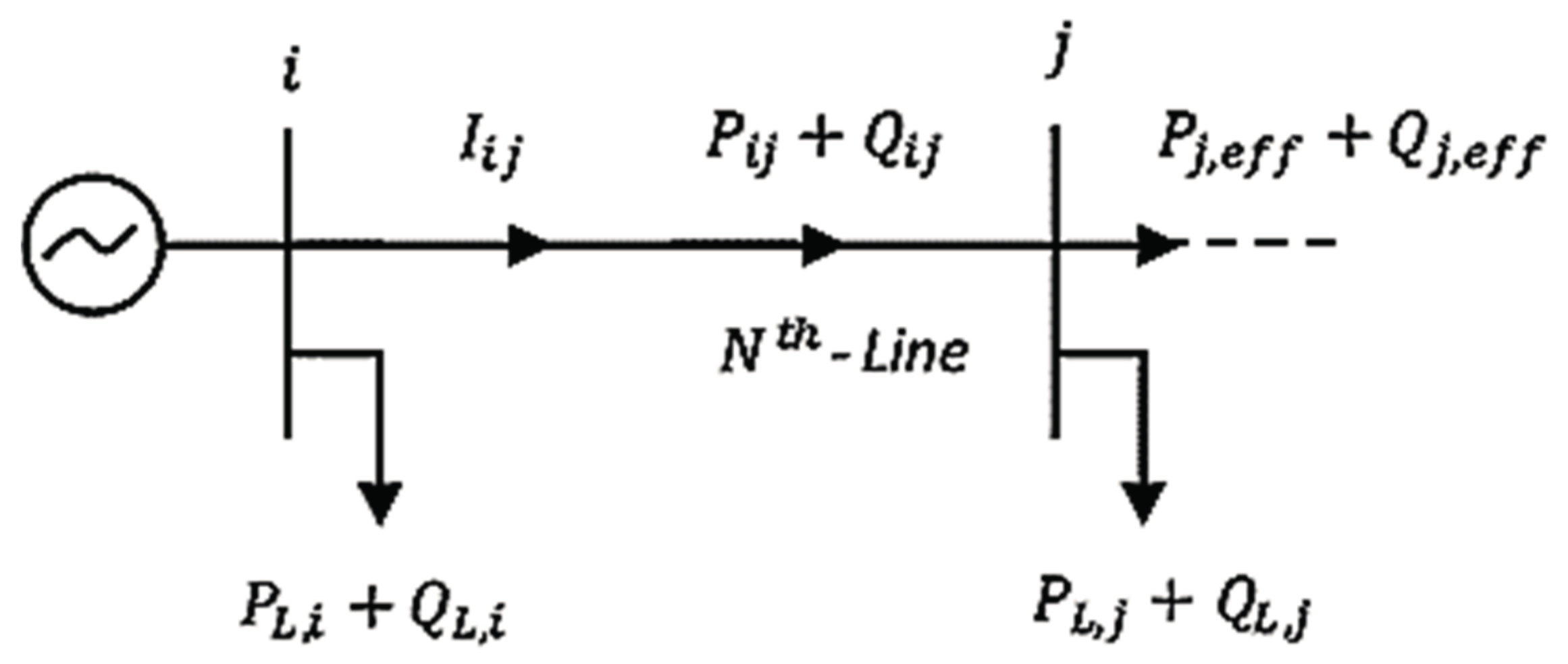
3.1. Formulation of Power Flow

The Backward/Forward Sweep (BFS) algorithm is employed for power flow computations [22,23]. Figure 6 shows the sample of a distribution network, considering a line ‘N’ is connected between two buses ‘i’ and ‘j’.

The analysis of BFS method is performed including three-main steps, which rely on the Kirchhoff’s voltage and currents law (KVL and KCL, respectively). The three steps comprise: (i) Back-ward Sweep; (ii) Forward Sweep; and (iii) Nodal current analysis. These steps are based upon convergence achievements if the maximum mismatch between voltages is less than the epsilon tolerance “error” (In this work, ‘ε_t’ is considered = 0.000001). After convergence, the active and reactive power losses for radial distribution system can be estimated easily. The determinations of BFS power flow are as follows:

The active (P_ij) and reactive (Q_ij) powers that flow through branch ‘N’ from node ‘i’ to node ‘j’ can be derived in (i) backwards sweep direction from the last node and are given as:

$$P_{ij}=P_j^{\prime }+R_{ij}\frac{(P_j^{\prime 2}+Q_j^{\prime 2})}{V_j^2}$$

(1)

$$Q_j^{\prime }=Q_j^{\prime }+X_{ij}\frac{(P_j^{\prime 2}+Q_j^{\prime 2})}{V_j^2}$$

(2)

where, $P_{ij}^{\prime }=P_j+P_{Lj}$ and $Q_{ij}^{\prime }=Q_j+Q_{Lj}$. The $P_{Lj}$ and $Q_{Lj}$ are loads and they are connected at node ‘j’.

The voltage magnitude and angle at each node are evaluated in (ii) Forward Sweep direction. Consider a voltage $V_i\angle {\delta }_i$ at node ‘i’ and $V_j\angle {\delta }_j$ at node ‘j’, then the (iii) the nodal current analysis flowing through the branch ‘N’ having an impedance, $Z_{ij}=R_{ij}+j{X}_{ij}$ connected between ‘i’ and ‘j’ is given as:

$$I_{ij}=\frac{(V_i\angle {\delta }_i-V_j\angle {\delta }_j)}{R_{ij}+j{X}_{ij}} \mathrm{and},$$

(3)

$$I_{ij}=\frac{(P_i-j{Q}_i)}{V_i\angle -{\delta }_i}$$

(4)

From Equations (3) and (4) the voltage at bus “j” can be estimated as follows:

$$V_j={[V_i^2-2*(P_i{R}_{ij}+j{Q}_i{X}_{ij})+(R_{ij}^2+X_{ij}^2)*\frac{(P_i^2+Q_i^2)}{V_i^2}]}^{0.5}$$

(5)

The magnitude and the phase angle equations can be employed respectively in (ii) a forward sweep direction for finding the voltage and angle of all nodes of radial distribution system. The active and reactive power losses of line ‘N’ between buses ‘i’ and ‘j’ can be evaluated as:

$$P_{Loss(ij)}=R_{ij}\frac{(P_{ij}^2+Q_{ij}^2)}{V_i^2}$$

(6)

$$Q_{Loss(ij)}=X_{ij}\frac{(P_{ij}^2+Q_{ij}^2)}{V_i^2}$$

(7)

The total real power loss of radial distribution system can be estimated as:

$$P_{TLoss}={\displaystyle \sum _{j=1}^N{P}_{Loss(ij)}}$$

(8)

where, ‘N’ is the number of the branches, i = 1: nb, and ‘nb’ is the number of buses.

3.2. Voltage Stability Index Analysis

The Voltage Stability Index (VSI) is considered as one of the indices that are employed to check the power system security level [29]. VSI is evaluated from the load flow for all the nodes of the grid and the values are arranged in ascending order. To avoid the potential of voltage collapse, the VSI of nodes should be maximized by installing RDGs based on optimum location and capacity in distribution network. However, the VSI evaluation at each node was presented in details by [19] as follows:

$$VS{I}_{(j)}={\left|V_i\right|}^4-4\times {[P_{j,eff}\times X_{ij}-Q_{j,eff}\times R_{ij}]}^2-4\times [P_{j,eff}\times R_{ij}-Q_{j,eff}\times X_{ij}]\times {\left|V_i\right|}^2$$

(9)

3.3. Power Loss Calculation with DG Units

After installing RDGs units in the distribution network, the power losses through a line section in Figure 1 can be derived as:

$$P_{DG,Loss(ij)}=R_{ij}\frac{(P_{DG(ij)}^2+Q_{DG(ij)}^2)}{V_i^2}$$

(10)

The total power loss of RDGs is estimated by the following Equation (11):

$$P_{DG,TLoss}={\displaystyle \sum _{j=1}^N{P}_{DG,Loss(ij)}}$$

(11)

3.4. Power Loss Index

The ratio of total power loss with RDGs units to the total power loss without RDGs is deemed the power loss index $\Delta P{l}_{DG}$ [21] and is estimated as follows:

$$\Delta P{l}_{DG}=\frac{P_{DG,TLoss}}{P_{TLoss}}$$

(12)

The integration of RDGs reduces the total system power loss. The minimizing of the total power loss can be realized by minimizing $\Delta P{l}_{DG}$.

3.5. Voltage Deviation Index

The voltage deviation index $\Delta V_{Dev}$ [21] can be derived as:

$$\Delta V_{Dev}=\max \left(\frac{V_1-V_i}{V_1}\right),\forall i= 1,2, \dots , nb (\mathrm{Number} \mathrm{of} \mathrm{buses})$$

(13)

3.6. Minimization of Total Operational Cost

The operational cost minimization is considered one of the RDGs installation merits in the distribution networks [21]. The operational cost is concluded in two components. The first one is considered as the active power supplied from the substation. The second one is the cost of active power supplied by RDGs units that are integrated. The total operating cost (TOC) can be minimized by the following formula:

$$TOC=(C_1{P}_{DG,TLoss})+(C_2{P}_{T,DG})$$

(14)

where, C₁ and C₂ are the cost coefficient of real power supplied by substation and RDGs in $/kW. $P_{T,DG}$ is the total active power drawn from installed RDGs.

The net operating cost $\Delta OC$ that can be minimized is derived in the following expression:

$$\Delta OC=\frac{TOC}{C_2{P}_{T,DG}^{\max }}$$

(15)

3.7. Objective Function

The objective function in this work is deemed as multi-objective function for minimizing the power loss, voltage deviation, and total operating cost of the distribution network. It is illustrated by the following function:

$$Min(f)=\min ({\lambda }_1\Delta P{l}_{DG}+{\lambda }_2\Delta V_{Dev}+{\lambda }_3\Delta OC)$$

(16)

where:

$${\displaystyle \sum _{k=1}^3{\lambda }_k=1.0}\wedge {\lambda }_k\in [0,1]$$

(17)

These parameters ${\lambda }_k$ are considered as the weight factors of the objective function [21]. The proposed objective function is minimized depending on the following constraints:

• The voltage at each bus $V_i$ in radial system must be kept within the acceptable maximum $V_{\max }$(1.05) and minimum $V_{\min }$(0.95) limits, as follows:

  $${}_{V_{\min }\le V_{\left(i\right)}\le V_{\max }}$$

  (18)
• The limits of voltage drop can be considered as the following Equation:

  $$\left|V_1-V_i\right|\le \Delta V_D^{\max }$$

  (19)
• The total RDGs size $P_{T,DG}^{}$ is kept within $P_{T,DG}^{\max }$ and $P_{T,DG}^{\min }$ as follows [21]:

  $$P_{T,DG}^{\max }\le P_{T,DG}^{}\le P_{T,DG}^{\min }$$

  (20)
• The apparent power line flow ‘S’ through the lines is limited by its maximum rating as:

  $$S_{l(i)}\le S_{l(i)}^{rated}$$

  (21)
• For stable operation of distribution system, the Voltage Stability Index (VSI) values of each node should be near to unity as [19]:

  $$VS{I}_{(j)}>0$$

  (22)

3.8. Sensitivity Factors Analysis

Loss sensitivity factor (LSF) is implemented to deduce the critical buses for the RDGs unit’s locations. Considering a distribution line connected among ‘i’ and ‘j’ buses and a load of $P_{j,eff}+j{Q}_{j,eff}$ represent the total effective active and reactive power supplied beyond bus ‘j’ as shown in Figure 6. Therefore, the active power losses through lines beyond bus ‘j’ can be determined as follows:

$$P_{lineloss(ij)}=R_{ij}\frac{(P_{j,eff}^2+Q_{j,eff}^2)}{V_j^2}$$

(23)

Now, the loss sensitivity factor ($LS{F}_{(ij)}$) can be evaluated by considering the first derivative of $P_{lineloss(ij)}$ in Equation (23) with respect to the active power load $P_{j,eff}$ as in the following expression [17,21]:

$$LS{F}_{(ij)}=\frac{\partial P_{lineloss}}{\partial P_{j,eff}}=\frac{2\times P_{j,eff}\times R_{ij}}{V_j^2}$$

(24)

The voltage sensitivity factor (VSF) is evaluated by the ratio of the base case voltage magnitudes at buses V_(i) to the minimum limit of voltage (0.95 p.u.). The LSF results are sorted in descending order for all the lines of the given system. The buses with largest values of LSF and smallest values of VSF (i.e., <1.01) are elected as the candidate buses for RDGs placement.

4. Optimization Techniques

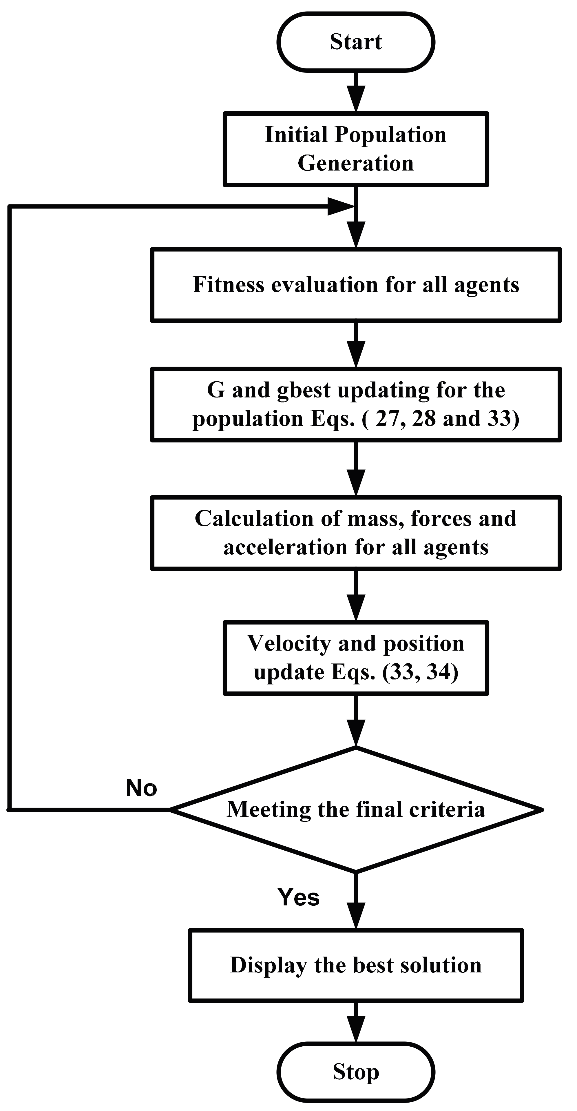
4.1. A Hybrid PSOGSA Optimizer

The Hybrid PSOGSA approach is constructed with the incorporation of PSO and Gravitational Search Algorithm (GSA) [30]. In PSO, Kennedy and Eberhart [31,32] provided PSO that is considered as an evolutionary technique. The PSO was deduced from social behavior of bird flocking. It uses a number of particles as candidate solutions which fly around in the search space to find best solution. To modify and update the position of each particle in PSO have to deem the current velocity and position, the distances of ‘pbest’ and ‘gbest’. The mathematical model of PSO can be concluded as the following Equations [30]:

$${\nu }_{it}^{1+ti}=w\times {\nu }_{it}^{ti}+c_1\times r_1[pbes{t}_{it}^{ti}-x_{it}^{ti}]+c_2\times r_2[gbes{t}_{it}^{ti}-x_{it}^{ti}]$$

(25)

$$x_{it}^{1+ti}=x_{it}^{ti}+\Delta t\times {\nu }_{it}^{ti+1}$$

(26)

where ${\nu }_{it}^{ti}$ is the velocity of particle ‘it’ at iteration ‘ti’, Positive constants ‘c₁’ and ‘c₂’ are the weighting factors, which are the acceleration constants responsible for varying the particle speed towards pbest and gbest, respectively. Variables ‘r₁’ and ‘r₂’ are two random numbers generated in the range [0, 1]. Equation (26) provides the position update, depending on its previous position and its velocity, considering Δt = 1. In Equation (25) consists of three parts, first part introduces exploration ability of PSO. Second and third parts are considered as private thinking and cooperation of particles respectively [30]. In Equation (25), after calculating the velocities, the position of masses can be evaluated in Equation (26). The iteration of process will continue updating the particles’ position until achieving the PSO target.

In GSA, Rashedi et al. [33] implemented GSA as a novel heuristic optimization tool. The theory of this technique is deduced from Newton’s gravitational force behavior which is called “action at a distance” [30,33]. GSA can be consummated as a combination of agents “selected solutions” whose have masses proportional to their value of fitness function. These masses are attracted between each other during generations. During the masses processes, the heavier masses that have a huge attraction force are possibly near the global optimum attract the other masses proportional to their distances.

For modeling GSA mathematically, it is assumed that the system starts with randomly ‘Na’ agents that are placed in the search space. The gravitational force is acquainted from ‘k’ to ‘l’ at time ‘t’ as follows [33]:

$$F_{lk}^d(t)=G(t)\frac{M_{pl}(t)\times M_{ak}(t)}{R_{lk}(t)+\epsilon }(x_k^d(t)-x_l^d(t))$$

(27)

where G(t) is gravitational constant at time ‘t’, $M_{ak}$ is the active gravitational mass, $M_{pl}$ is passive gravitational mass, $\epsilon$ is a small constant, and $R_{lk}(t)$ is Euclidian distance between two agents ‘l’ and ‘k’.

The gravitational constant is evaluated as:

$$G(t)=G_o\times exp(-\alpha \times iter/max itare)$$

(28)

where G_o and α are initial value and descending coefficient respectively, ‘iter’ is current iteration, and ‘$\max itare$’ is maximum number of iterations.

The total force, which affects agent ‘l’ is deduced as:

$$F_l^d(t)={\displaystyle {\sum }_{k=1,l\ne k}^{N_a}{r}_k{F}_{lk}^d}(t)$$

(29)

where, ‘d’ is dimension of problem space, $r_k$ is a random number [30]. The acceleration of an agent is deduced according to the law of motion as the following:

$$a{c}_l^d(t)=\frac{F_l^d(t)}{M_l(t)}$$

(30)

where, $M_l$ is the mass of object ‘l’ during time ‘t’.

The velocity and position of agents are deduced as follows:

$$ve{l}_l^d(t+1)=r_l\times ve{l}_l^d(t)+a{c}_l^d(t)$$

(31)

$$x_l^d(t+1)=x_l^d(t)+ve{l}_l^d(t+1)$$

(32)

The GSA process is operated according to the previous equations from Equation (28) to Equation (32), and then it will be finished until reaching to the end of its criterion.

In this paper and according to Mirjalili in [30], the PSO and GSA are hybridized based on a low-level co-evolutionary heterogeneous hybrid. The big advantage in this new approach, is that they run in parallel. The basic concept of PSOGSA is to merge the ability of social thinking in PSO (gbest) with the local search capability (acceleration of all agents) of GSA $a{c}_l(t)$. Moreover, in hybrid mechanisms, PSO using its exploring feature pending the subsequent stages based on the social thinking in the method, and the GSA using its exploiting feature in the beginning stages of search process based on the local search in the method. Agents here are represented as distributed generation power sizes $P_{DG(j)}$ that can be evaluated based on Equation (33):

$$V_l(t+1)=w\times V_l(t)+c_1^{\prime }\times r\times a{c}_l(t)+c_2^{\prime }\times r\times (gbest-X_l(t))$$

(33)

where, $V_l(t)$ is the velocity, $c_1^{\prime }$, $c_2^{\prime }$ and $w$ are considered as weighting factors. The positions of these particles (agents) are updated based on Equation (34):

$$X_l(t+1)=X_l(t)+V_l(t+1)$$

(34)

These positions are considered as the RDGs allocations.

In this paper, the PSOGSA is worked according to the flow chart operation illustrated in Figure 7.

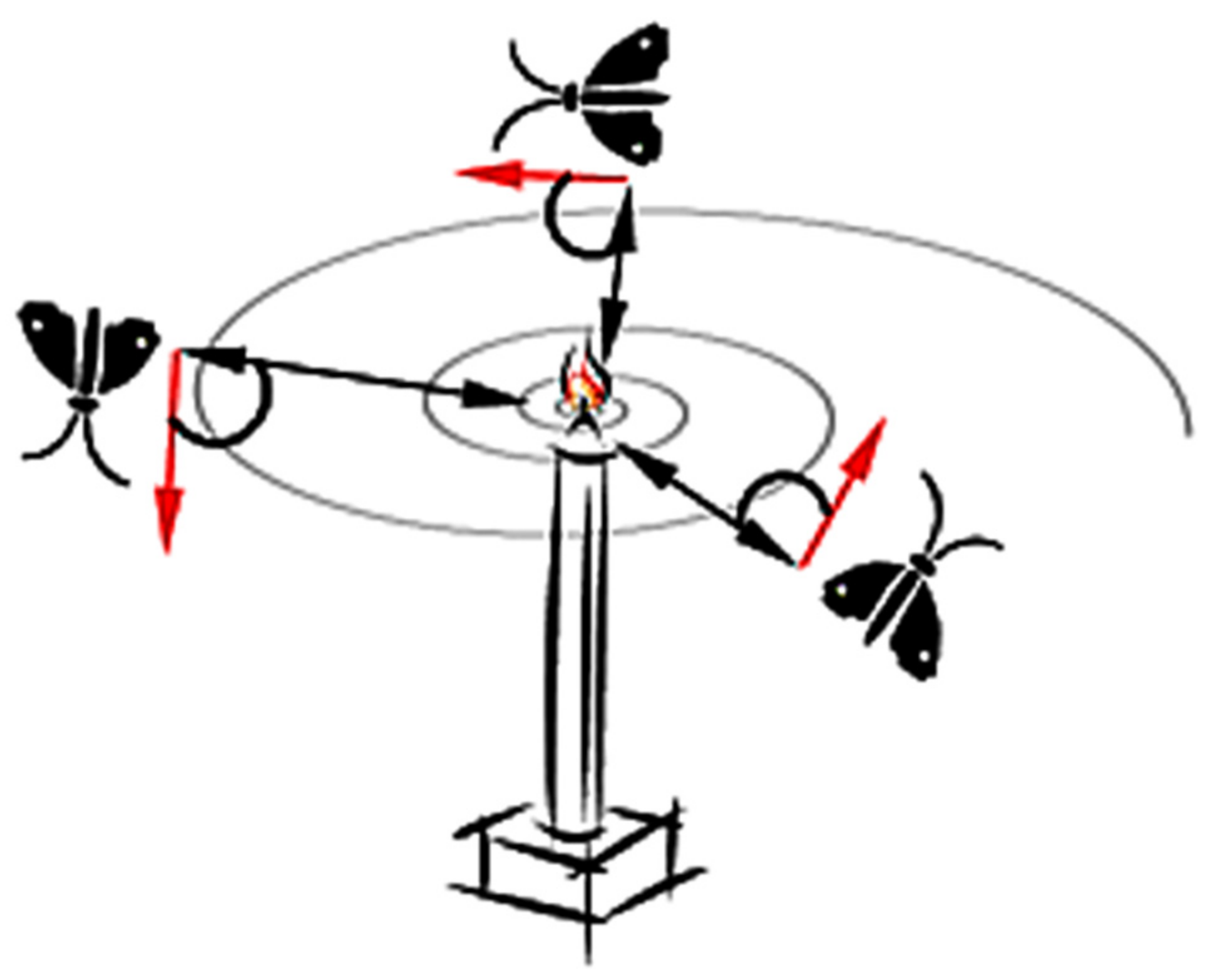
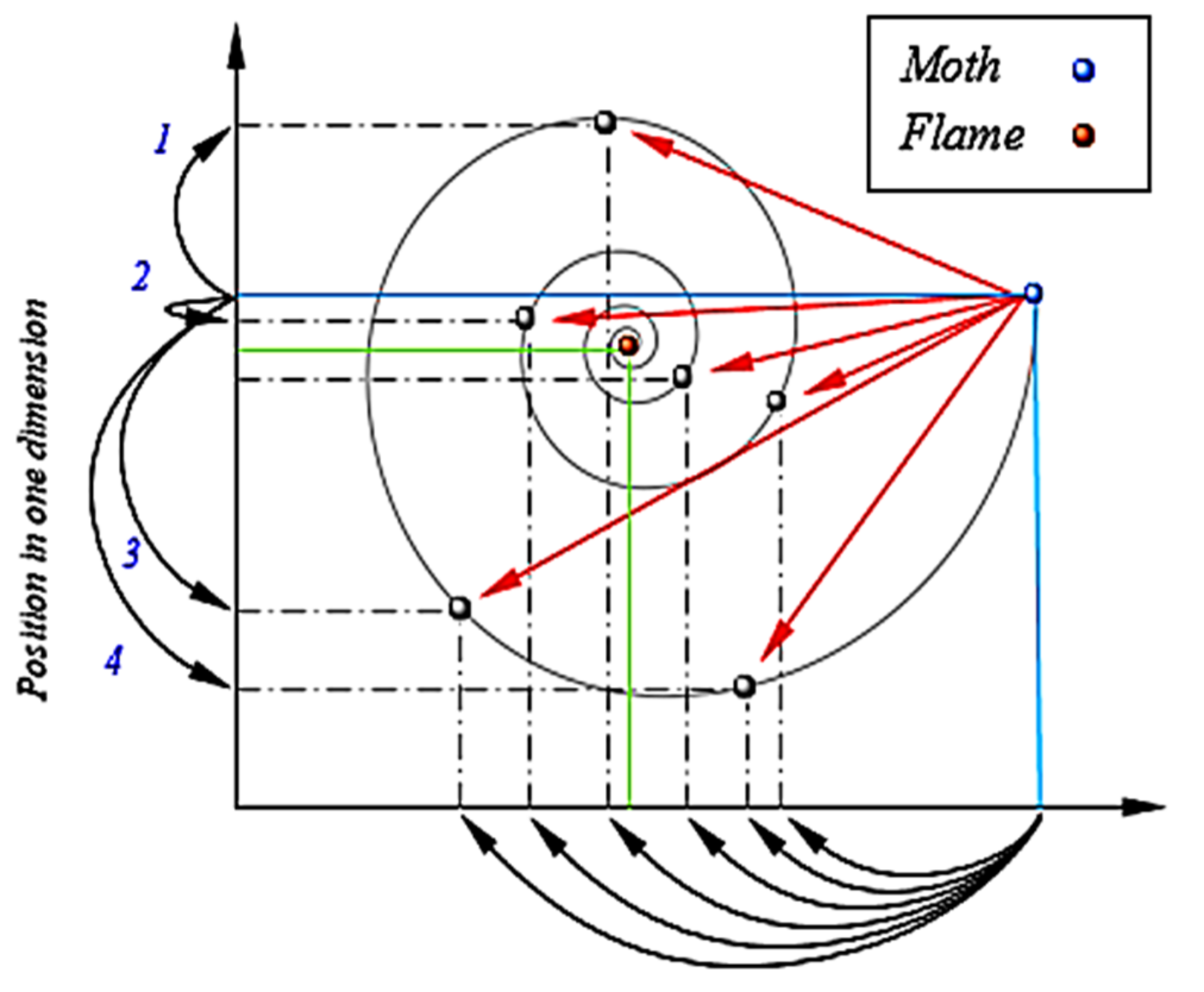
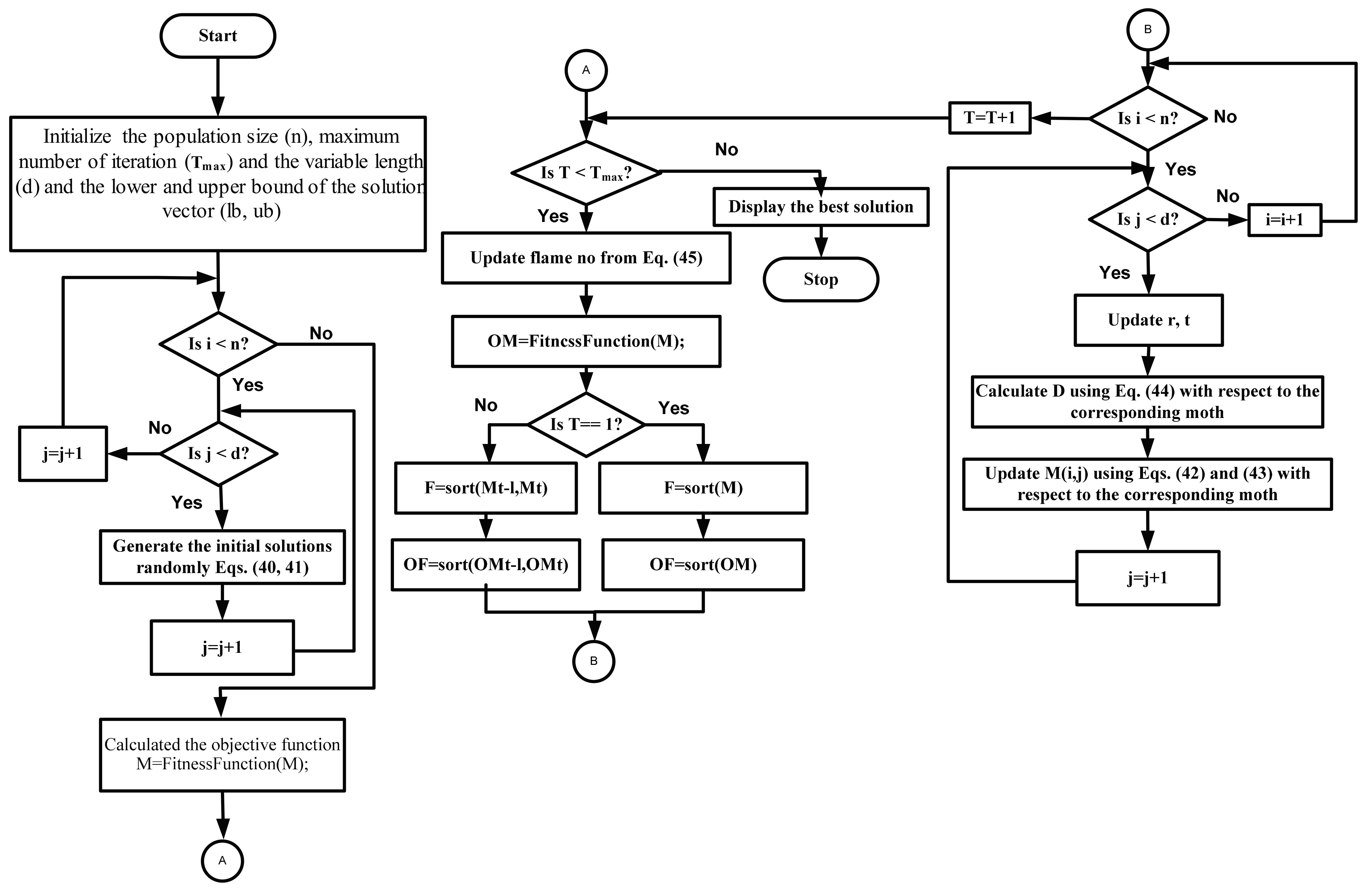
4.2. The MFO Optimizer

Mirjalili was the first to propose the sophisticated Moth-Flame Optimization (MFO) algorithm in 2015 [34]. MFO is a new population-based algorithm. Moths are fancy insects that are inspired by special navigation mechanism in the night called transverse orientation. These moths fly at night by preserving a fixed angle with respect to the moon, this special mechanism is very useful for moving in a straight streak particularly the source of light is away. When the source of light is nearby, moths fly spirally around it and lastly converge towards it after just a few refinements as introduced in Figure 8 [34].

Moths and flames are the main components of the MFO algorithm. Moreover, both of moths and flames have been considered as a solution. However, during each iteration, there is a difference in the way of treatment and updating of them. The moths are genuine search agents that move around the search space, however, flames are the best position of moths that acquired so far. Consequently, flames can be deemed as flags that are dropped by moths when searching the search space. Therefore, each moth searches around a flame and updates it in the case of finding a better solution. Through this process, a moth never fails to reach its best solution [34].

Because the MFO algorithm is deemed as a population-based algorithm, the following matrix is the set of moths (M):

$$M=\left(\begin{array}{ccc}{m}_{1,1}& \dots & m_{1,d}\\ ⋮& \ddots & ⋮\\ m_{n,1}& \dots & m_{n,d}\end{array}\right)$$

(35)

The values of the corresponding objective function for all moths $OM$ are stored in the following matrix [34]:

$$OM=\left(\begin{array}{c}O{M}_1\\ O{M}_2\\ ⋮\\ O{M}_n\end{array}\right)$$

(36)

where, the OM is represented as fitness function of moths (M).

Therefore, and similar to the moth’s matrix, the following matrix is considered the flames (F) matrix:

$$F=\left(\begin{array}{ccc}{F}_{1,1}& \dots & F_{1,d}\\ ⋮& \ddots & ⋮\\ F_{n,1}& \dots & F_{n,d}\end{array}\right)$$

(37)

Furthermore, fitness values of flames (OF) are stored as:

$$OF=\left(\begin{array}{c}O{F}_1\\ O{F}_2\\ ⋮\\ O{F}_n\end{array}\right)$$

(38)

The overall structure of the MFO procedure including three-tuple approximation function can be written as follows [34]:

$$MFO=\left(I,P,T\right)$$

(39)

The initialization function “I” that produces a random population of moths and values of their corresponding objective function is defined as:

$$M\left(i,j\right)=\left(ul\left(i\right)-ll\left(i\right)\right)\cdot rand()+ll(i)$$

(40)

$$OM=FitnessFunction(M)$$

(41)

where, $ul$ and $ll$ introduce the upper and lower limits of the variables respectively.

Once the initialization is finished, the ‘P’ function is run till the ‘T’ termination function is satisfied. The main function ‘P’ moves the moths around the search space. As stated earlier, the transverse coordination of moths is considered the main inspiration of the MFO algorithm. Consequently, the logarithmic spiral function is selected as the main updated mechanism of the position of each moth with respect to the flame.

The moth position regarding a flame is updated as:

$$M_i=S(M_i,F_j)$$

(42)

The logarithmic spiral for the MFO technique is written as follows:

$$S\left(M_i,F_j\right)=D_i\cdot e^{bt}\cdot cos\left(2\pi t\right)+F_j$$

(43)

where, $M_i$ indicates the ith moth, $F_j$ is the jth flame, and S is the spiral function. $D_i$ is the distance of the ith moth for the jth flame, b is a constant for describing the form of the logarithmic spiral, and t is a random number in [r, 1]. Thence, r is the adaptive convergence constant that linearly decreases from −1 to −2 to fast-track convergence around the flames over the path of iterations.

D is estimated using Equation (44):

$$D_i=\left|F_j-M_i\right|$$

(44)

The spiral equation is to assure that a moth flies around a flame and not in the space between them. The updated moth positions around the flame are illustrated in Figure 9. Exploration takes place once the next position lies outside the space between the moth and the flame that can be shown by the arrows labeled as 1, 3, and 4. Whilst, the exploitation occurs when the next position lies inside the space between the moth and flame that can be illustrated in arrow labeled as 2. Equation (45) illustrates that the number of flames adaptively decreases over the iterations to assure the balance between the exploration and exploitation. Therefore, the positions of the moths have been updated only regarding the best flame in the final steps of iterations:

$$flame no=round\left(N_f-l\times \frac{N_f-1}{T_{max}}\right)$$

(45)

where, ‘l’ is the current number of iteration, $N_f$ is the maximum number of flames, and $T_{max}$ is the maximum number of iterations.

After all, the overall operation steps in this article of the developed MFO can be represented in Figure 10. As debated before the ‘P’ function is carried out until the ‘T’ function returns true. After terminus the ‘P’ function, the best moth is returned back as the best acquired approximation of the optimum. For optimization problem, $OM$ is the objective function and represents the optimum solution of RDGs installation.

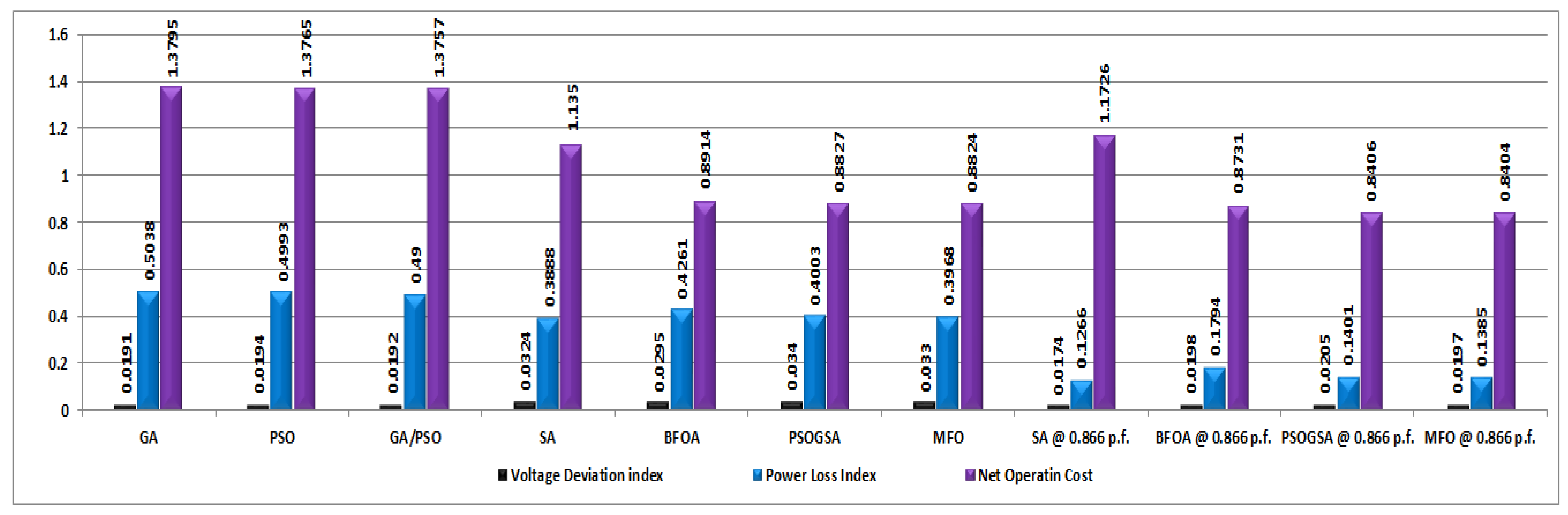
5. Simulation Results

The proposed PSOGSA and MFO algorithms have been executed via the MATLAB package (MathWorks, Natick, MA, USA). The proposed PSOGSA and MFO methodologies have been tested on two 12.66 kV IEEE standard radial distribution networks, which they are 33-bus and 69-bus [21]. The weighting factors ${\lambda }_1$, ${\lambda }_2$ and ${\lambda }_3$ of the main objective function are submitted as 0.5, 0.4, and 0.1, respectively [21]. The cost coefficients C₁ and C₂ in the equation of TOC are chosen as 4 $/kW and 5 $/kW according to [21], where C₂ is the maintenance and installation costs of RDGs units. The choosing of the candidate buses from LSF is deduced depending on VSF values. The buses that have the VSF values below 1.01 p.u. are considered as the candidate buses for RDGs location. Then the algorithms of PSOGSA and MFO provide the optimal RDGs sizing and placement from the chosen buses. To study the performance and efficiency of the proposed PSOGSA and MFO on 33-bus and 69-bus IEEE distribution network, the operation of RDGs is chosen at two different power factors unity and 0.866 that are supposed as two types of RDGs according to [17,21]. Type-A at unity power factor is capable of injecting only active power (e.g., photovoltaic “PV” system) and Type-C is capable of injecting both active and reactive power (e.g., wind turbine “WT”) that is considered in this section at optimal power factor 0.866. The proposed optimization algorithms are compared with other optimization techniques and methods as follows. The parameters definitions of the proposed methodologies PSOGSA and MFO are introduced in

Table 1. The definition of used parameters.

Maximum Iteration = 20 (MFO)	Number of Search Agents = 30 (MFO)
$0\le P_{DG}\le 1500$ kW, step size 50 kW	$c_1^{\prime }$= 0.5, $c_2^{\prime }$=1.5 (PSOGSA)
maximum iteration = 20 (PSOGSA)	population size = 30 (PSOGSA)
GO = 1 (PSOGSA)	α = 23 (PSOGSA)

, in addition other system parameters.

In our Egyptian case study, two scenarios at the maximum peak load level are considered as case study also. In scenario-I and scenario-II, it is supposed to integrate the PV system at unity PF or WT system at 0.866 respectively as mentioned before with 33-bus and 69-bus IEEE distribution systems. The optimum allocation of these RDGs types on MEDN case study is implemented based on the superior one from the comparison of MFO and PSOGSA techniques. The numerical results illustrate the superiority of the proposed PSOGSA and MFO methodologies in the following sections.

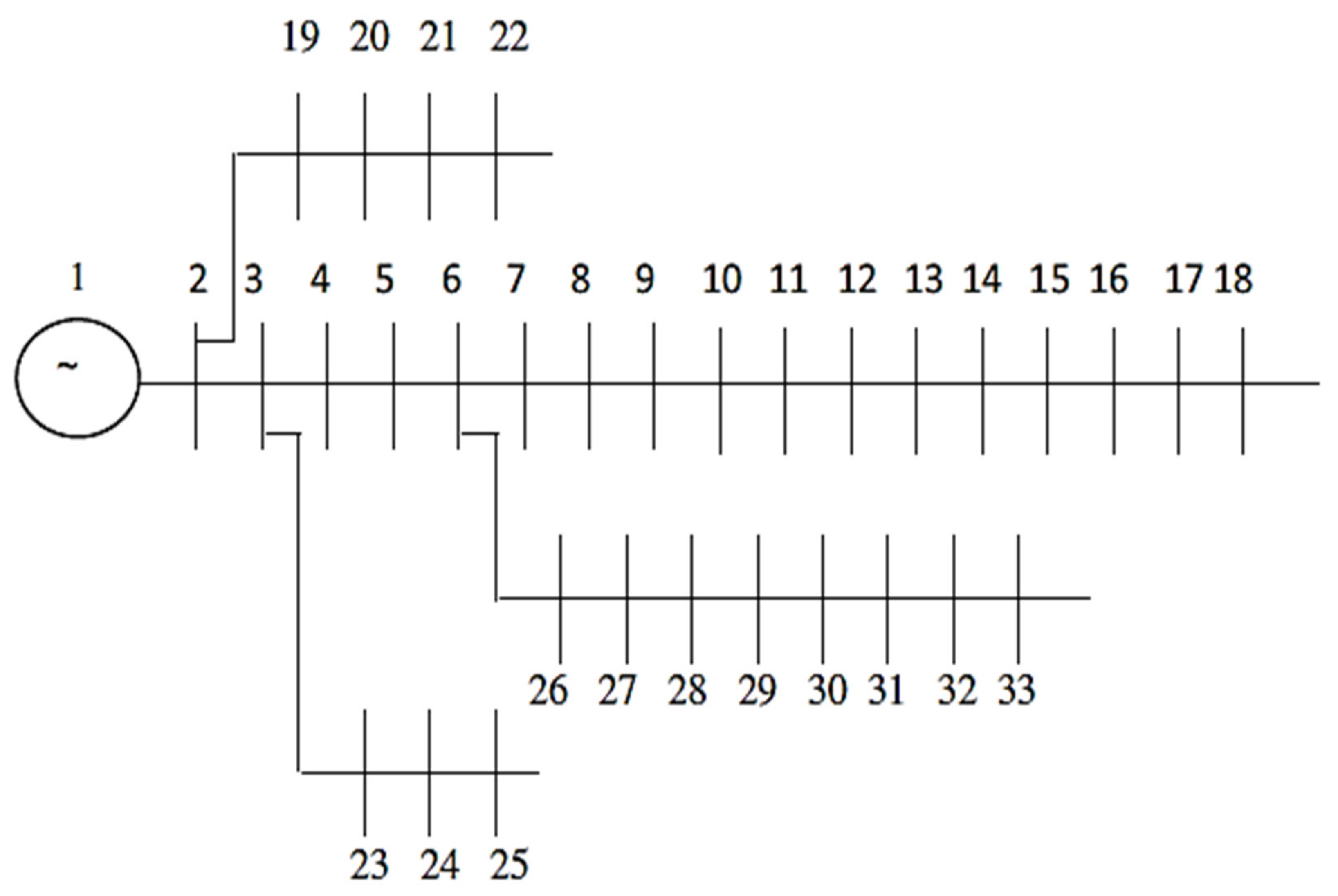
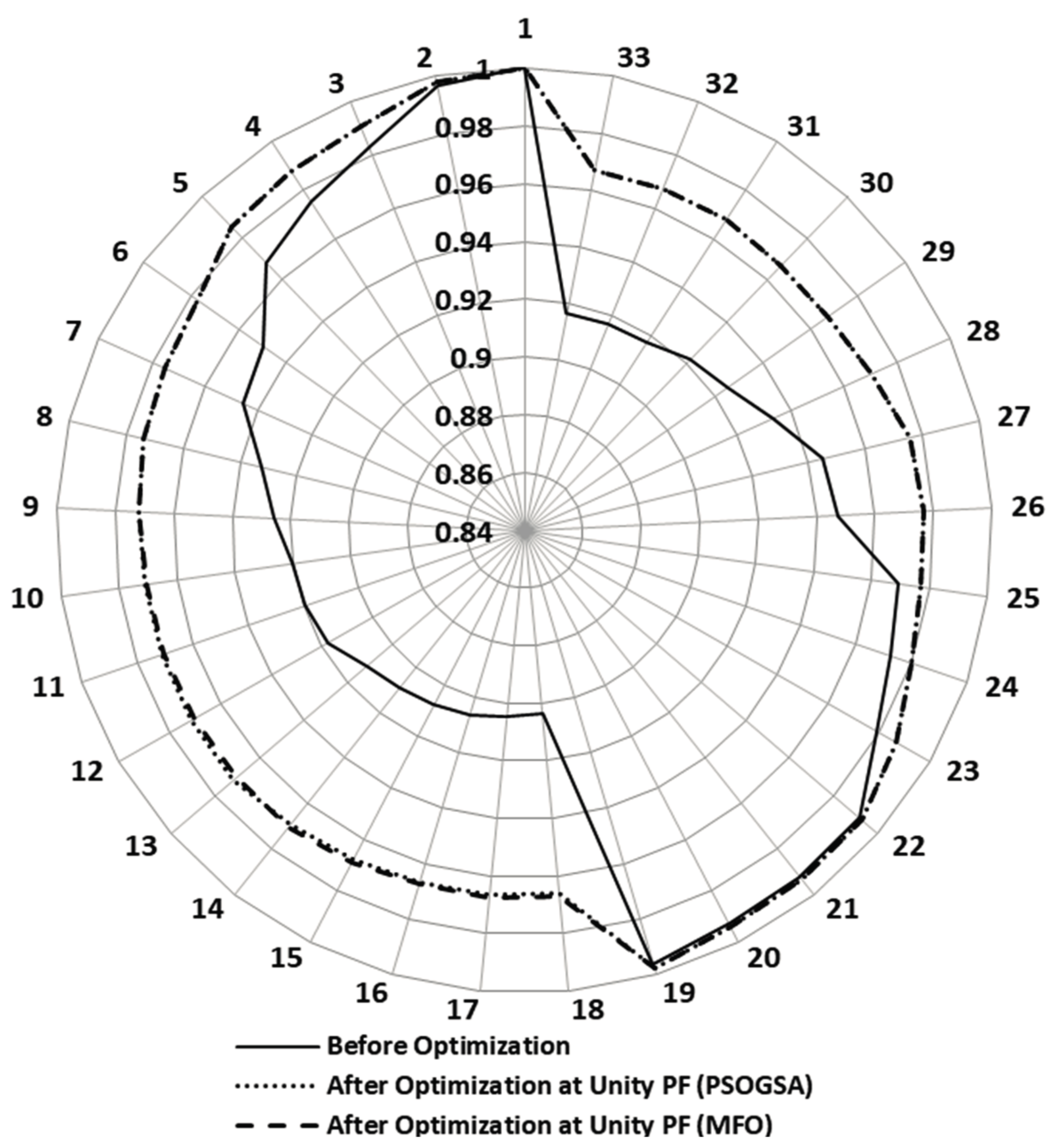
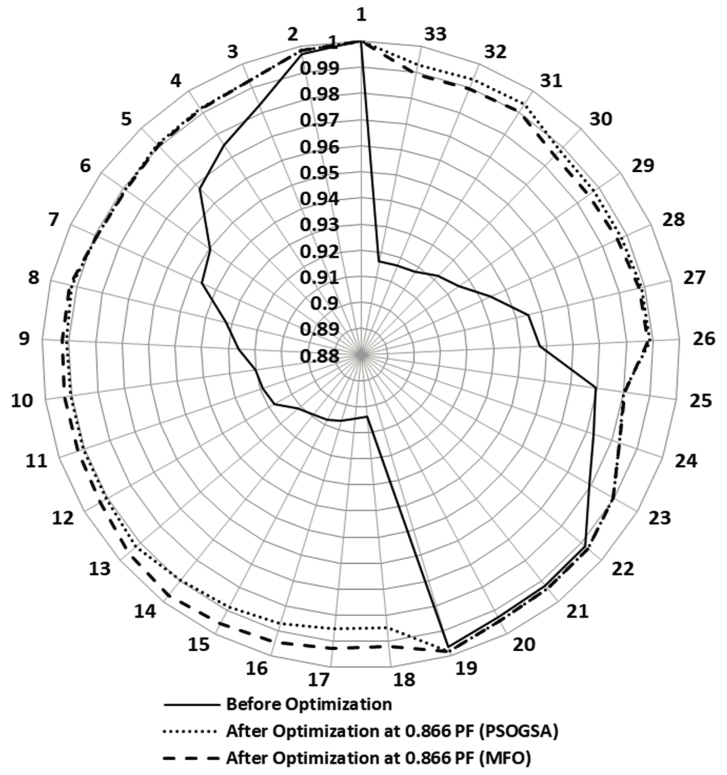
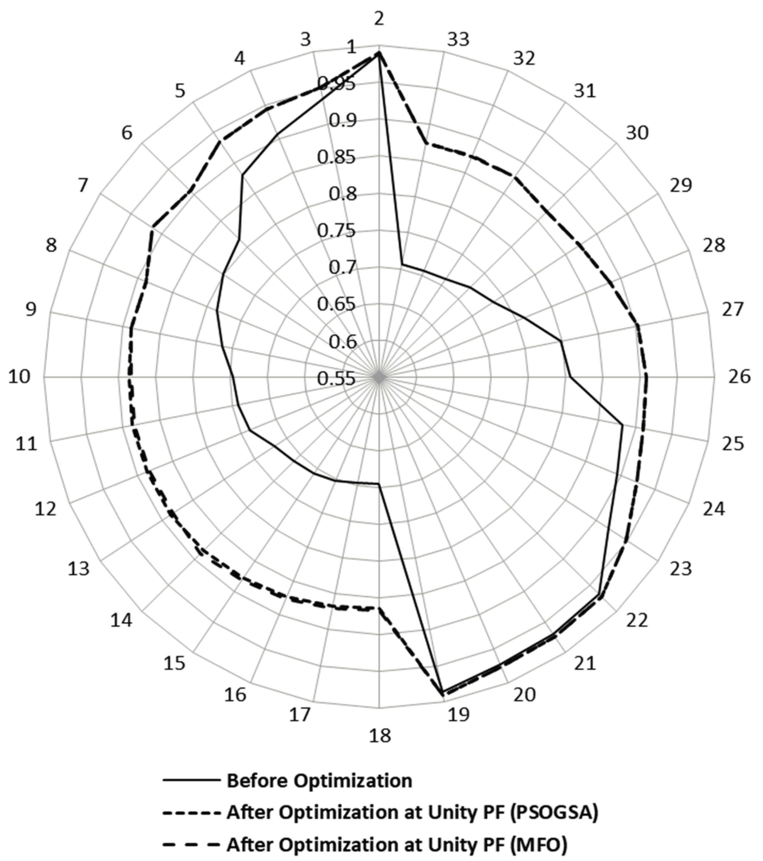
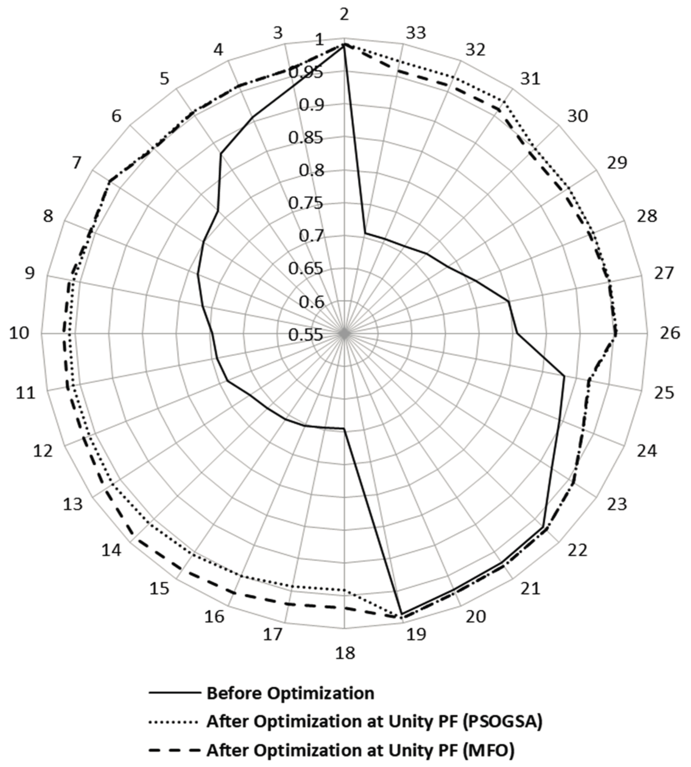
5.1. The Results of the 33-Bus IEEE Distribution System

The proposed methodologies are performed on 33-bus radial distribution test system which the rated voltage of this test model is 12.66 kV as shown in Figure 11 [21]. The results of highest LSF with lowest VSF values of 33-bus (i.e., VSF < 0.01) are presented in

Table 2. The results of LSF and VSF of 33-bus IEEE distribution network.

33 Bus	LSF1	VSF1
6	0.0233	0.9995
8	0.0215	0.9814
28	0.0121	0.9827
9	0.0101	0.9747
13	0.0099	0.9595
10	0.0095	0.9685
29	0.0087	0.9740
31	0.0061	0.9659
30	0.0046	0.9703
27	0.0034	0.9947
14	0.0032	0.9571
17	0.0029	0.9520
12	0.0028	0.9660
7	0.0028	0.9957
26	0.0026	0.9974
15	0.0024	0.9556
16	0.0024	0.9541
11	0.0016	0.9676
32	0.0010	0.9513

Bold items represent the first 11 rows of LSF1 and VSF1 results that will be selected by PSOGSA and MFO.

. After applying the optimization PSOGSA algorithm, the most critical buses from the first 11 rows in

Table 3. The results of 33-bus IEEE distribution network at unity PF (PV type).

Items	Before Optim.	After Optimization at Unity PF (PV System) for 33-Bus
		BSOA [17]	GA [19]	PSO [19]	GA/PSO [19]	SA [20]	BFOA [21]	Proposed PSOGSA	Proposed MFO
Total losses (kW)	210.98	89.05	106.30	105.35	103.4	82.03	89.90	84.3330	83.7133
Loss reduction %	-	57.792	49.61	50.06	50.99	61.12	57.38	60.03	60.32
Vmin (p.u.), bus	0.9038 (18)	0.9554 (18)	0.9809 (25)	0.9806 (30)	0.9808 (25)	0.9676 (14)	0.9705 (29)	0.9660 (18)	0.9670 (18)
VSImin (p.u.), bus	0.6672 (18)	NA	NA	NA	NA	NA	NA	0.8647 (18)	0.8677 (18)
Optimal location and size of RDGs (kW)		(13) 632	(11) 1500	(13) 981.6	(32) 1200	(6) 1112.4	(14) 652.1	(8) 400	(8) 450
	-	(28) 487	(29) 422.8	(32) 982.7	(16) 863	(18) 487.4	(18) 198.4	(13) 650	(14) 600
		(31) 550	(30) 1071.4	(8) 1176.8	(11) 925	(30) 867.9	(32) 1067.2	(31) 850	(31) 850
SDG,T (kVA)	-	1669	2994.2	2988.1	2988	2467.7	1917.6	1900	1900
RDGs Power Factor	-	unity	unity	unity	unity	unity	unity	unity	unity
TOC ($)	-	NA	15,396.2	15,361.9	15,353.6	12,666.6	9948.1	9837.3	9834.9
CPU time(s)/Iteration/N	-	24.95/150/13	NA	NA	NA	NA	NA	8.656/20/30	7.1/20/30

Bold items represent the numerical results based on PSOGSA and MFO.

, which have sufficient effects on the network with RDGs are identified as 8, 13, and 31. The optimal sizes for these critical buses are 400, 650, and 850 (kW), respectively, at unity power factor (PV system). The same buses are deduced at 0.866 PF (WT) with optimal size results of 450, 500, and 900 kW, respectively, and the total apparent power is 2136.25 kVA. Also, after applying the MFO optimization technique, the most critical buses are identified as 8, 14, and 31. The optimal sizes for these critical buses are 450, 600, and 850 (kW), respectively, at unity power factor (PV system). The same buses are introduced at 0.866 PF (WT) with optimal size results of 450, 600, and 800 kW, respectively, and the total apparent power is 2136.25 kVA. The PSOGSA and MFO results of 33-bus are shown in Table 3 and

Table 4. The results of 33-bus IEEE distribution network at 0.866 PF (WT type).

Items	Before Optim.	After Optim. Type (WT) for 33-Bus
		BSOA [17]	SA [20]	BFOA [21]	Proposed PSOGSA	Proposed MFO
Total losses (kW)	210.98	29.65	26.72	37.85	29.5083	29.2139
Loss reduction %	-	85.9465	87.33	82.06	86.013	86.153
Vmin (p.u.), bus	0.9038 (18)	0.9795 (25)	0.9826 (25)	0.9802 (29)	0.9798(25)	0.9803(25)
VSImin (p.u.), bus	0.6672 (18)	NA	NA	NA	0.9207(25)	0.9209(25)
Optimal location and size of RDGs (kW)		(13) 698	(6) 1197.6	(14) 679.8	(8) 450	(8) 450
	-	(29) 402	(18) 477.8	(18) 130.2	(13) 500	(13) 600
		(31) 658	(30) 920.5	(32) 1108.5	(31) 900	(31) 800
SDG,T (kVA)	-	2307.359	2997.5	2215.3	2136.25	2136.25
DGs Power Factor	-	0.86, 0.71, 0.7	0.866	0.866	0.866	0.866
TOC ($)	-	NA	13,086.3	9743.9	9368	9366.9
CPU time(s)/Iterations/N	-	56.5/200/18	NA	NA	10.2/20/30	9.3/20/30

Bold items represent the numerical results based on PSOGSA and MFO.

. From these tables of PSOGSA and MFO results, the values of installed capacity of active power and total apparent power for the proposed MFO are significantly small as compared with PSOGSA and other techniques with great increasing in the percentage reduction of TOC and power loss. In the case of the SA method and at unity PF, the total power loss is reduced to 82.03 kW with the TOC of 12,666.6$ i.e., 2831.7$ greater than the MFO, also BFAO has 9948.1$ of TOC i.e., 113.2$ greater than the MFO. At 0.866 PF, the TOC is minimized by the MFO to 9366.9$ which is less than the TOC of the SA, BFAO and PSOGSA methods respectively. In addition, the minimum voltage of BFAO and PSOGSA at 0.866 PF is lower than proposed algorithm MFO. The BSOA has results lower than MFO with both PV system and WT, and it is not considered the system costs in objective function formula. The MFO is faster than BSOA and PSOGSA according to the elapsed time(s) of the program operation for producing optimal solution. The elapsed time and the attitude of objective functions of MFO and PSOGSA illustrate the superiority of MFO than PSOGSA to find the optimum minimum objective function in small number of iterations as illustrated in Figure 12 and Figure 13. Figure 14 and Figure 15 show the effects of RDGs types’ integration on voltage profile for 33-bus system. Moreover, the voltage stability index profile by both RDGs types installation is illustrated in Figure 16 and Figure 17. This indicates that the proposed algorithms especially MFO technique efficiently with high accuracy predicts the optimum placement and capacity of RDGs with the maximum percentage of reduction in power loss and operating cost (TOC) and improving the voltage profile. Figure 18 illustrates the performance of all techniques as compared as PSOGSA and MFO. It is shown in Figure 18 that the voltage deviation index is reduced highly in techniques GA, PSO, GA/PSO, and BFAO, but net operating cost (ΔOC) and power loss index are higher than in the proposed algorithms. The SA technique decreased the power loss index, but $\Delta OC$ is greater than PSOGSA and MFO. In the terms of acceptable and quality solutions, the numerical results in tables and figures illustrate that the performance of MFO is faster and better as compared as PSOGSA and other techniques with PV system and WT.

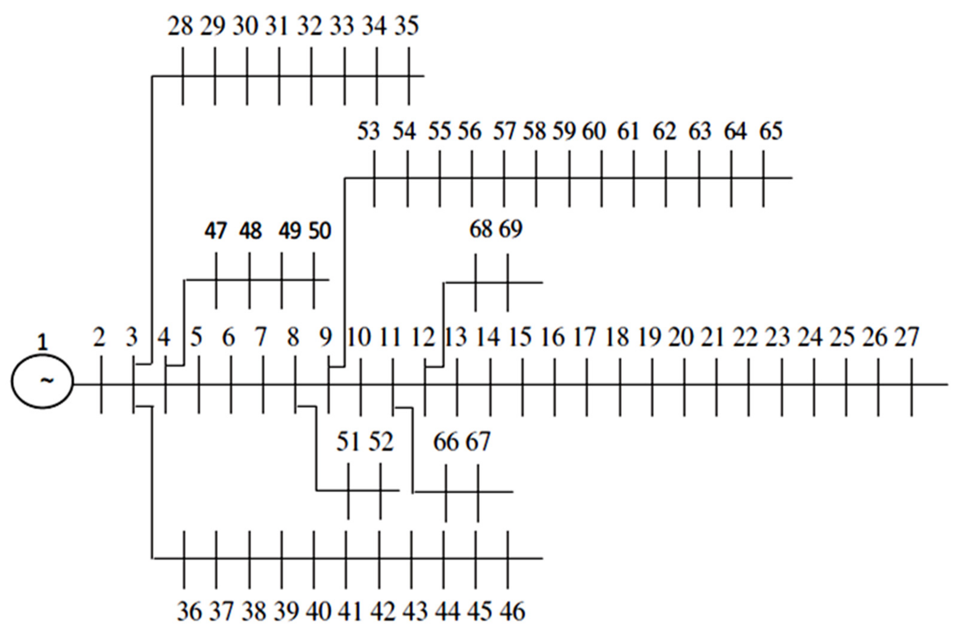
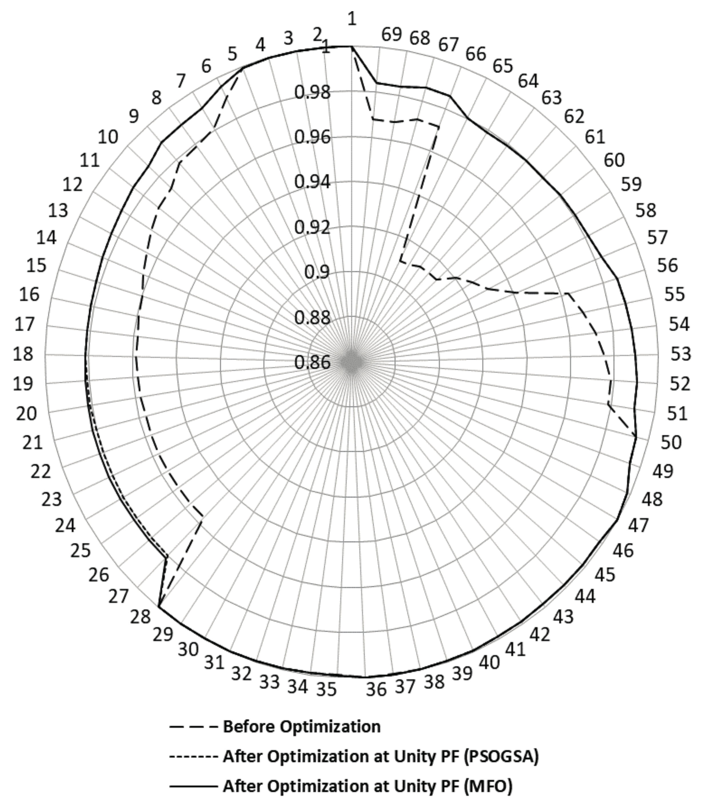
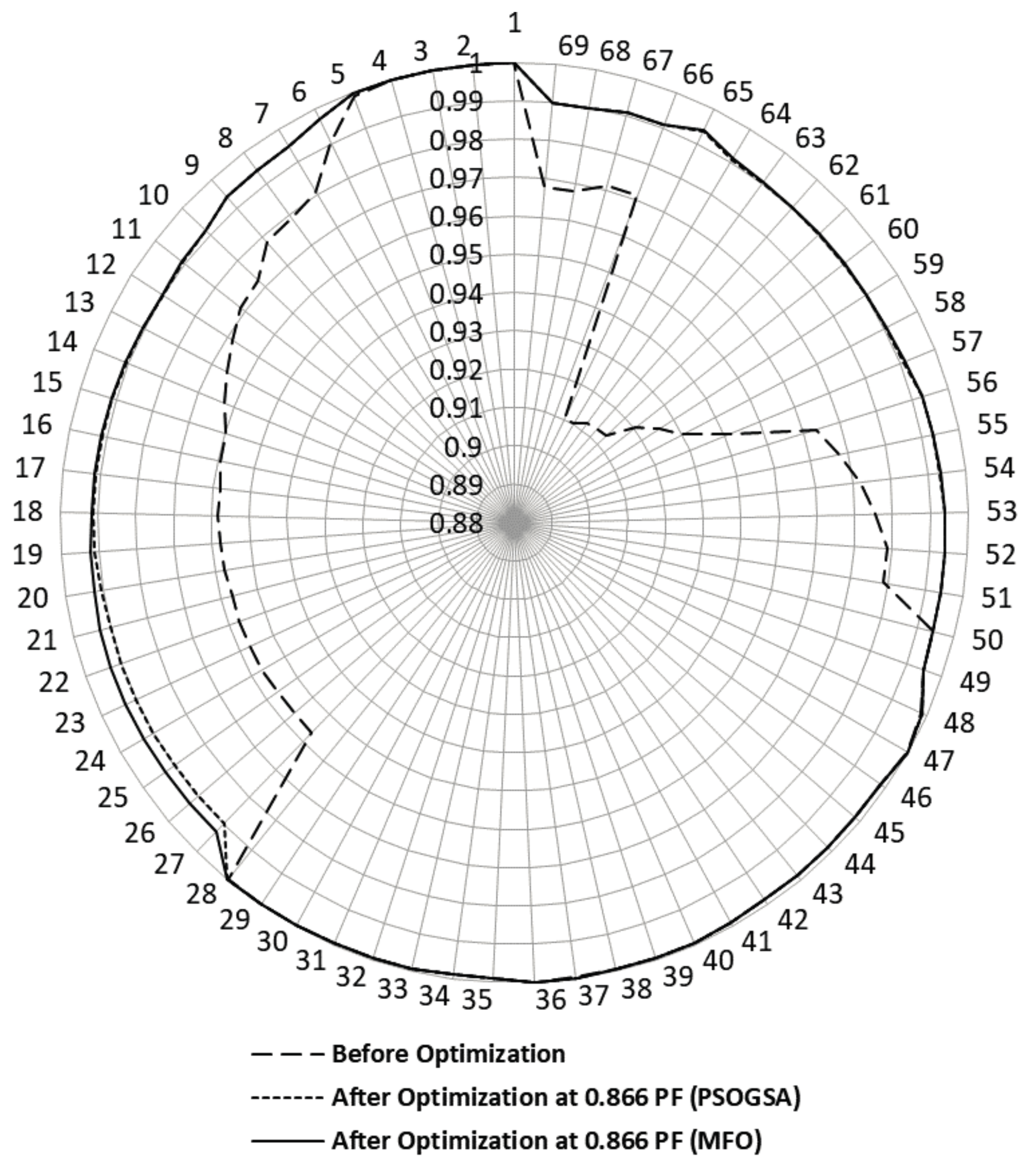
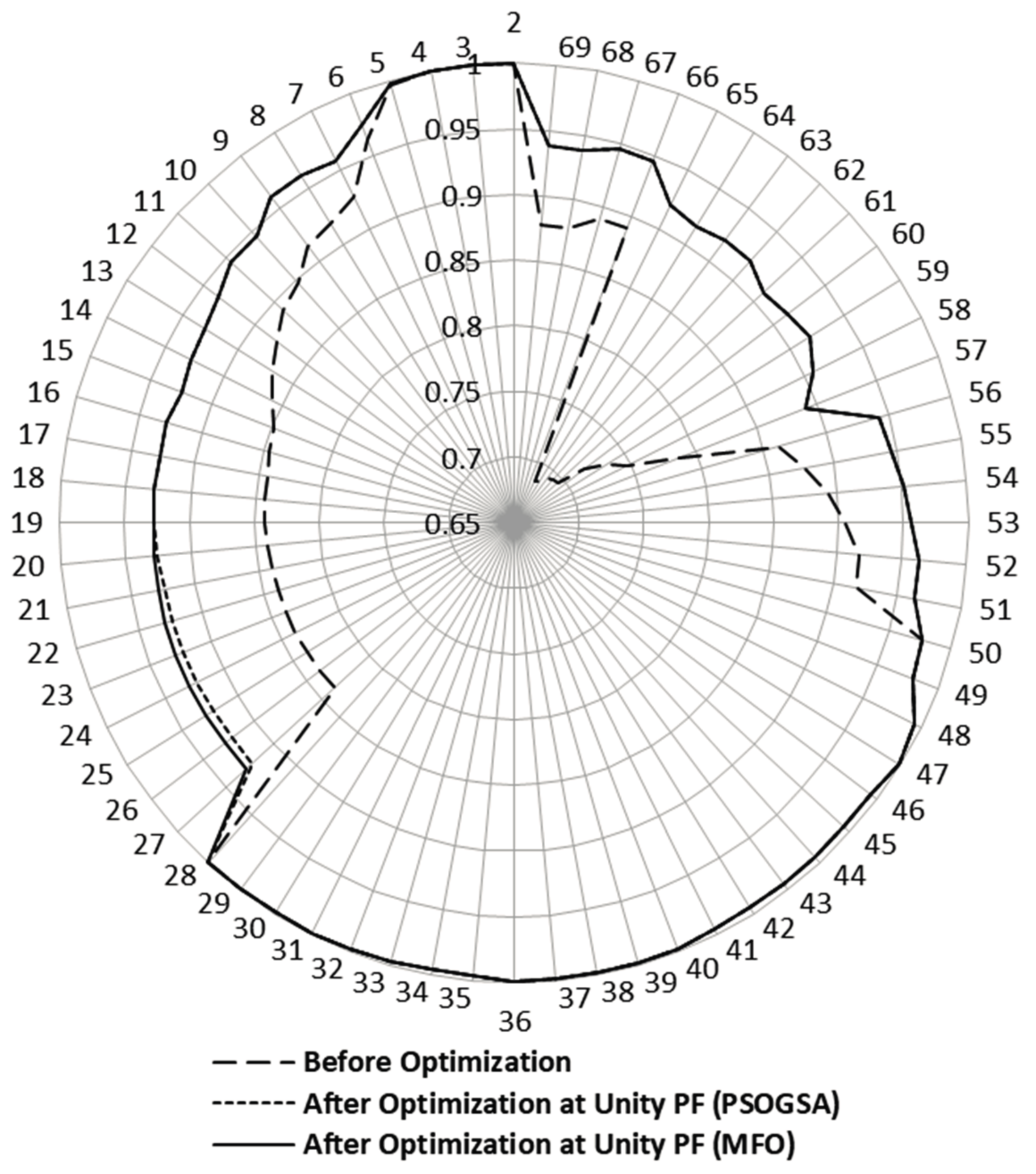
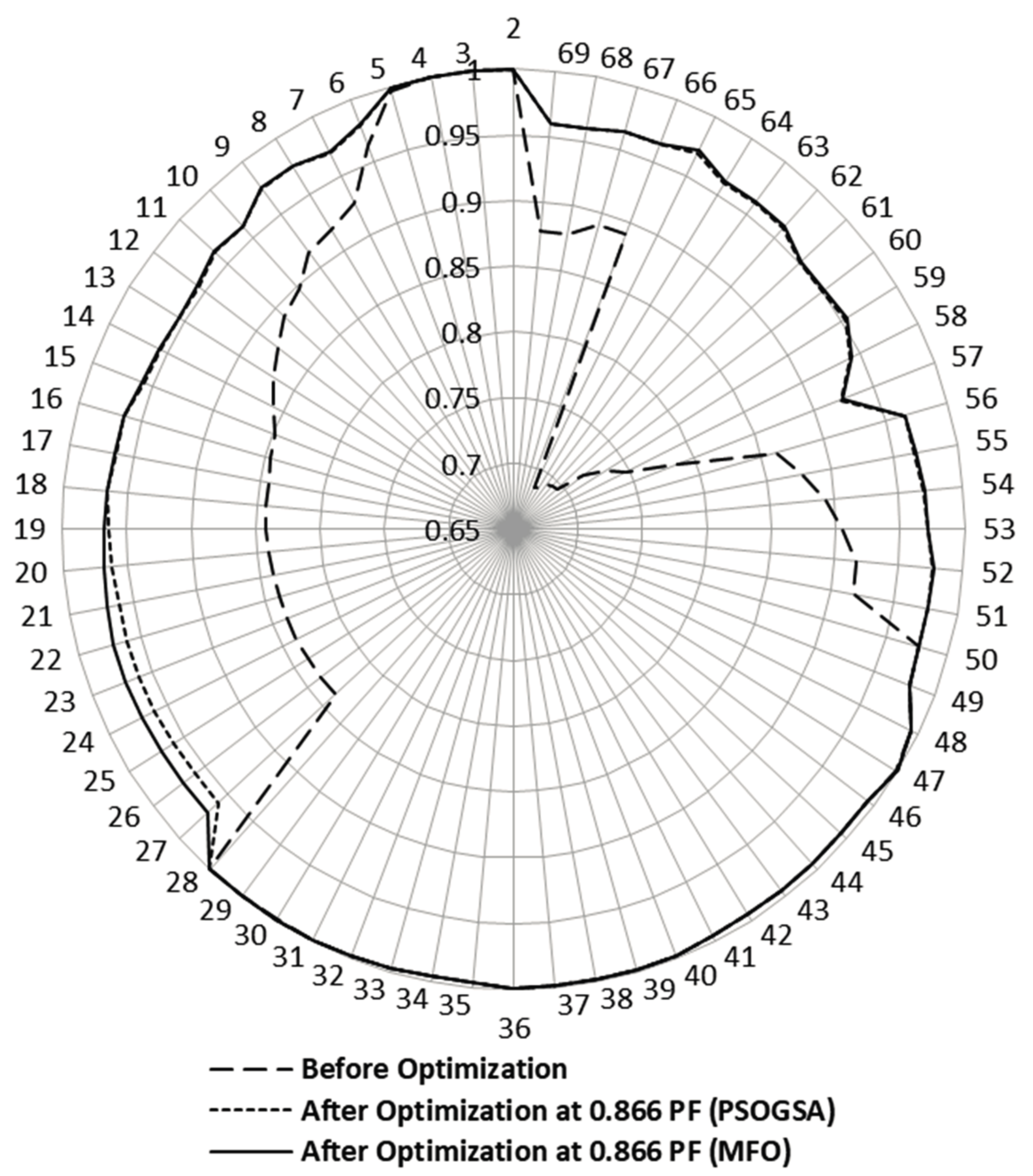
5.2. The Results of the 69-Bus IEEE Distribution System

The proposed methodologies are applied on a 69-bus radial distribution test system [21], where the rated voltage of this test model is 12.66 kV and the schematic diagram of the tested network is introduced in Figure 19.

Table 5. The results of LSF and VSF of 69-bus IEEE distribution network.

69 Bus	LSF2	VSF2
57	0.03725	0.9903
58	0.0188	0.9787
61	0.01186	0.9611
60	0.00888	0.9689
59	0.00737	0.9742
64	0.00306	0.9584
17	0.00151	1.0087
65	0.00093	0.9578
16	0.00091	1.0096
21	0.00082	1.0074
19	0.00079	1.0082
63	0.00062	0.9604
20	0.00051	1.0079
62	0.00046	0.9608
25	0.00029	1.0070
24	0.00026	1.0071
23	0.00012	1.0073
26	0.00012	1.0069
18	0.00002	1.0087

Bold items represent the first 11 rows of LSF2 and VSF2 results that will be selected by PSOGSA and MFO.

shows the LSF and VSF of 69-bus system. From PSOGSA results the most critical buses from the first 11-buses of LSF results are 17, 61, and 65 with optimal sizes of 300, 1450, and 300 (kW), respectively, at unity power factor (PV system). At 0.866 PF (WT), the optimal size results of PSOGSA for the same critical buses are 400, 1200, and 400 kW with total apparent power of 2000 kVA. Also, after applying the optimization MFO technique, the most critical buses are deduced as 21, 61, and 65 with the optimal sizes of 300, 1450, and 300 (kW), respectively, at unity power factor (PV system). The same buses are produced at 0.866 PF (WT) with optimal size results of 400, 1200, and 400 kW, respectively, and the total apparent power is 2000 kVA. The PSOGSA and MFO results of 69-bus are illustrated in

Table 6. The results of 69-bus IEEE distribution network at unity PF (PV type). Bold items represent the numerical results based on PSOGSA and MFO.

Items	Before Optim.	After Optimization at Unity PF (PV System) for 69-Bus
		GA [19]	PSO [19]	GA/PSO [19]	SA [20]	BFOA [21]	Proposed PSOGSA	Proposed MFO
Total losses (kW)	224.98	89	83.2	81.1	77.1	75.23	73.5895	73.4958
Loss reduction %	-	60.44	63.02	63.95	65.73	66.56	67.29	67.33
Vmin (p.u.), bus	0.9091 (65)	0.9936 (57)	0.9901 (65)	0.9925 (65)	0.9811 (61)	0.9808 (61)	0.9790 (64)	0.9792 (64)
VSImin (p.u.), bus	0.6855 (65)	NA	NA	NA	NA	NA	0.8906 (57)	0.8908 (57)
Optimal location and size of DGs (kW)		(21) 929.7	(61) 1199.8	(63) 884.9	(18) 420.8	(27) 295.4	(17) 300	(21) 300
	-	(62) 1075.2	(63) 795.6	(61) 1192.6	(60) 1331.1	(65) 447.6	(61) 1450	(61) 1450
		(64) 992.5	(17) 992.5	(21) 910.5	(65) 429.8	(61) 1345.1	(65) 300	(65) 300
SDG,T (kVA)	-	2997.4	2987.9	2988	2181.3	2088.1	2050	2050
DGs Power Factor	-	unity	unity	unity	unity	unity	unity	unity
TOC ($)	-	15,343	15,272.3	15,264.4	11,214.9	10,741.4	10,544	10,544
CPU time(s)/Iteration/N	-	NA	NA	NA	NA	NA	20.428/20/30	18.67/20/30

and

Table 7. The results of 69-bus IEEE distribution network at 0.866 PF (WT type).

Items	Before Optim.	After Optim. Type (WT) for 69-Bus
		SA [20]	BFOA [21]	Proposed PSOGSA	Proposed MFO
Total losses (kW)	224.98	12.26	12.9	12.8895	12.5361
Loss reduction %	-	92.77	94.26	94.27	94.43
Vmin (p.u.), bus	0.9091(65)	0.9885 (61)	0.9896 (64)	0.9897 (27)	0.9899 (68–69)
VSImin (p.u.), bus	0.6855 (65)	NA	NA	0.9222 (57)	0.9230 (57)
Optimal location and size of DGs (kW)		(18) 549.8	(27) 378.1	(17) 400	(21) 400
	-	(60) 1195.4	(65) 328.5	(61) 1200	(61) 1200
		(65) 312.2	(61) 1336.1	(65) 400	(62) 400
SDG,T (kVA)	-	2375.7	2358.7	2000	2000
DGs Power Factor	-	0.866	0.866	0.866	0.866
TOC ($)	-	10,352	10,265.1	10,052	10,050
CPU time(s)/Iteration/N	-	NA	NA	23.10/20/30	21.52/20/30

Bold items represent the numerical results based on PSOGSA and MFO.

. The values of installed capacity of active power and total apparent power for the proposed system are significantly small as compared as other techniques with great increase in the percentage reduction of TOC and power loss except power losses at 0.866 PF with SA method is less than PSOGSA and MFO. However, the worst minimum voltage of PSOGSA and MFO is a little higher than SA and BFOA at 0.866 PF. The MFO is faster than PSOGSA according to the elapsed time(s) of the program operation for deducing the optimal solutions. The elapsed time and the attitude of objective functions of MFO and PSOGSA illustrate the superiority of MFO than PSOGSA to find the optimum minimum objective function in a small number of iterations as illustrated in Figure 20 and Figure 21 at unity and 0.866 PF, respectively. Figure 22 and Figure 23 illustrate the effects of RDGs types’ integration on voltage profiles with PSOGSA and MFO for 69-bus system. Moreover, the voltage stability index profile by both RDGs types installation is shown in Figure 24 and Figure 25. The performance parameters at unity/0.866 of PSOGSA are as the following: voltage deviation index ($\Delta V_{Dev}$) = 0.021/0.0103, power loss index ($\Delta P{l}_{DG}$) = 0.3271/0.0573 and net operating cost ($\Delta OC$) = 0.9244/0.8812. Also, the performance parameters at unity/0.866 of MFO are as follows: voltage deviation index ($\Delta V_{Dev}$) = 0.0208/0.0101, power loss index ($\Delta P{l}_{DG}$) = 0.3267/0.0557 and net operating cost ($\Delta OC$) = 0.9244/0.8811. All results show the superiority and effectivity with a high performance and speed of the proposed MFO algorithm to get the optimal location and capacity of RDGs units in different distribution networks.

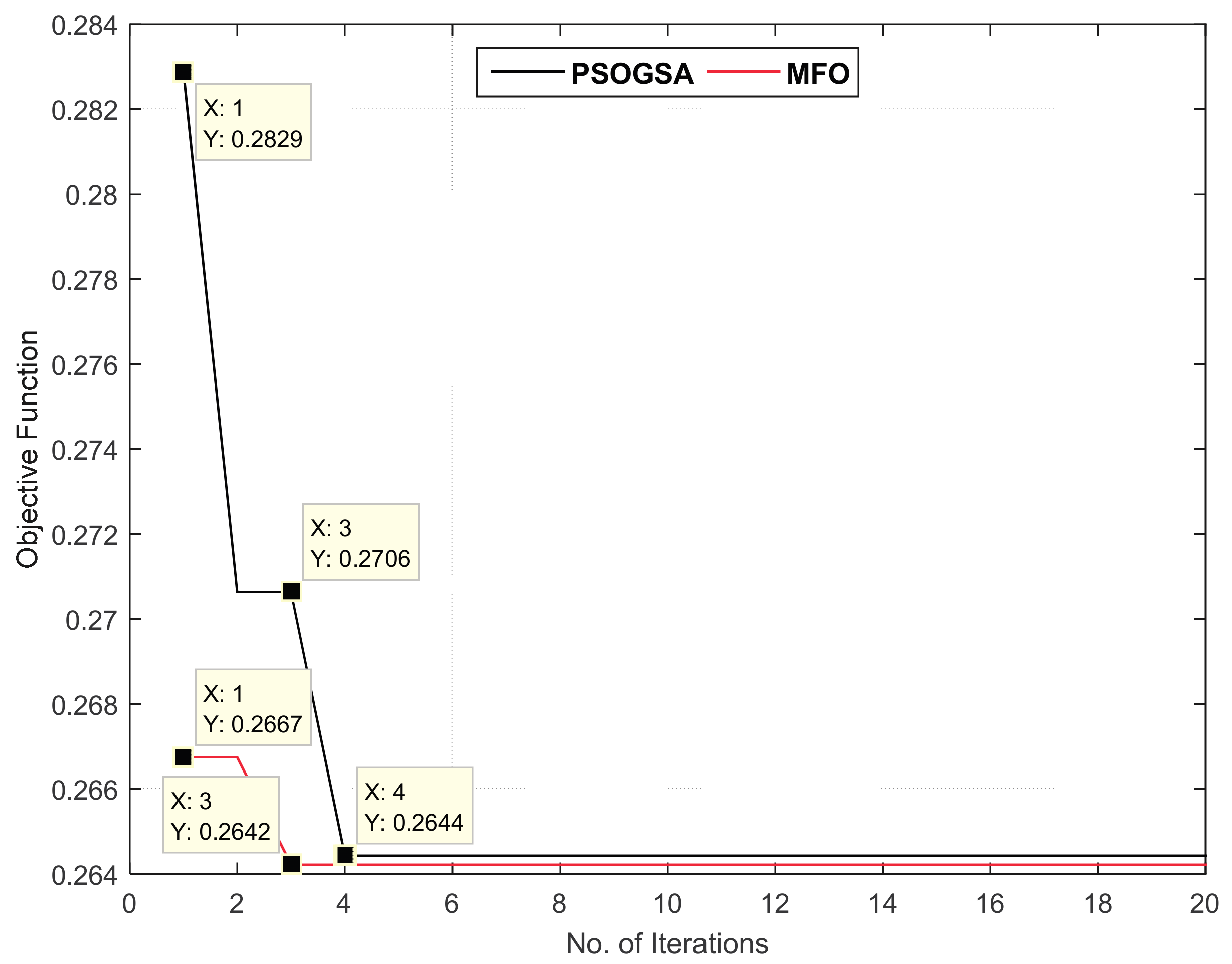
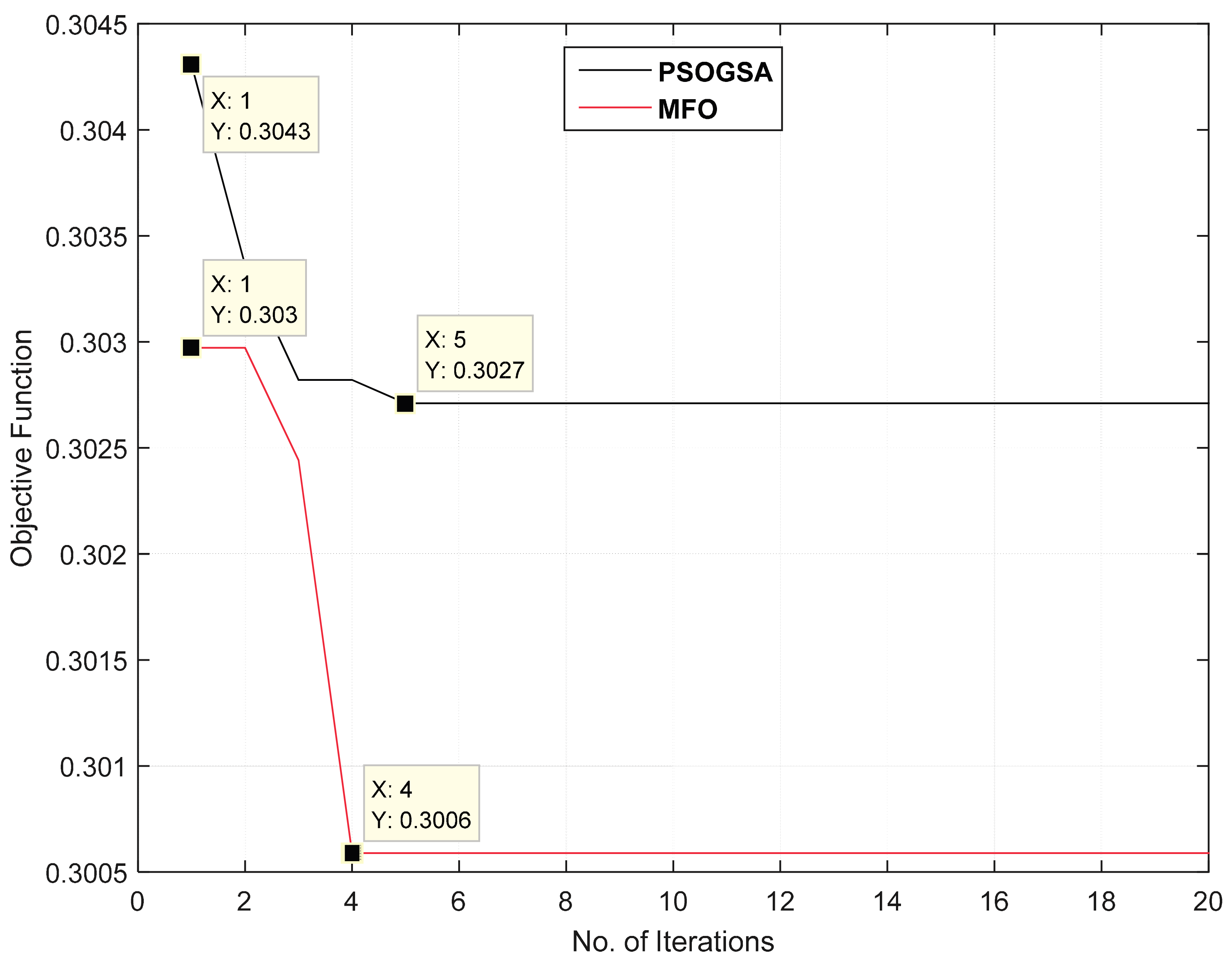
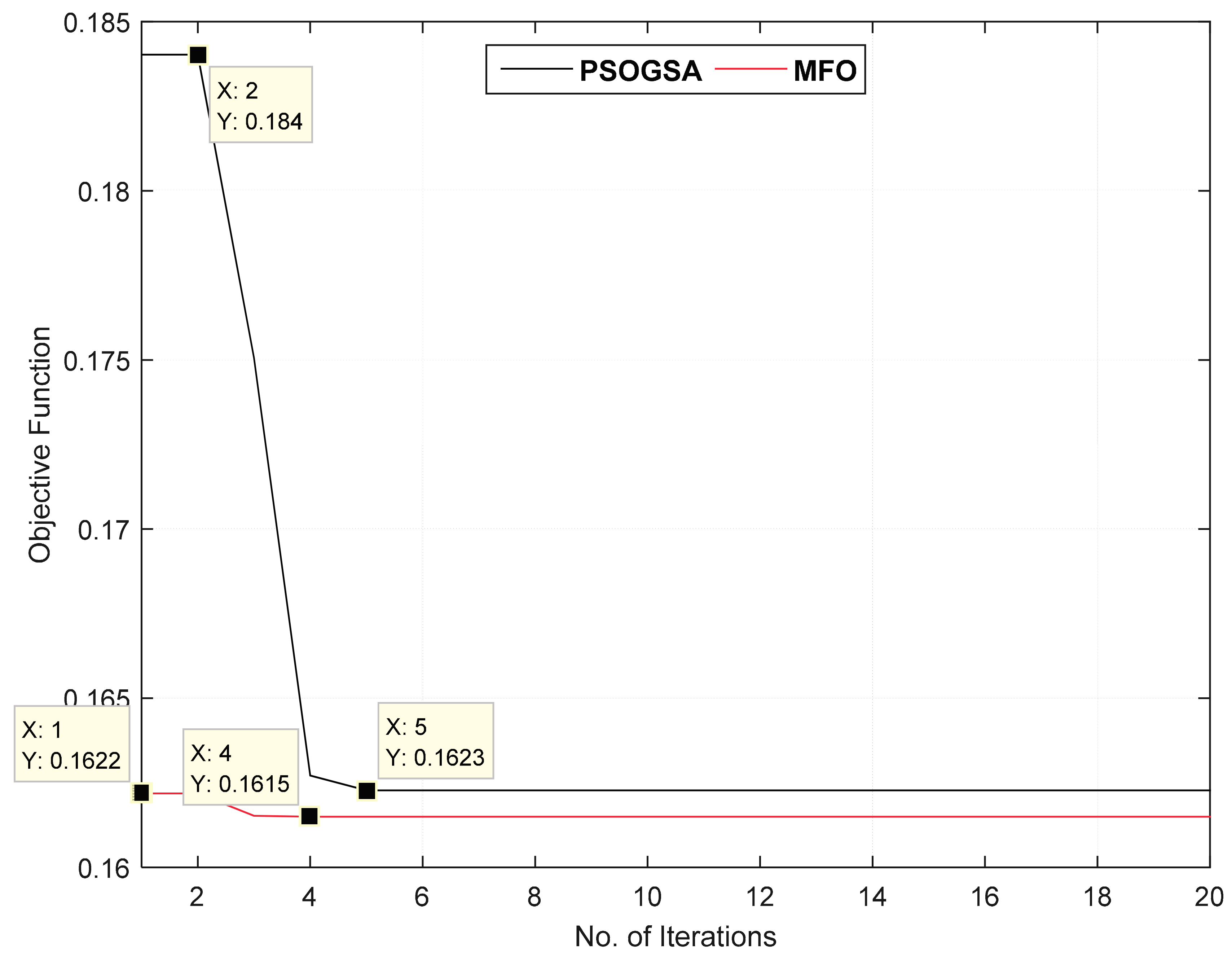
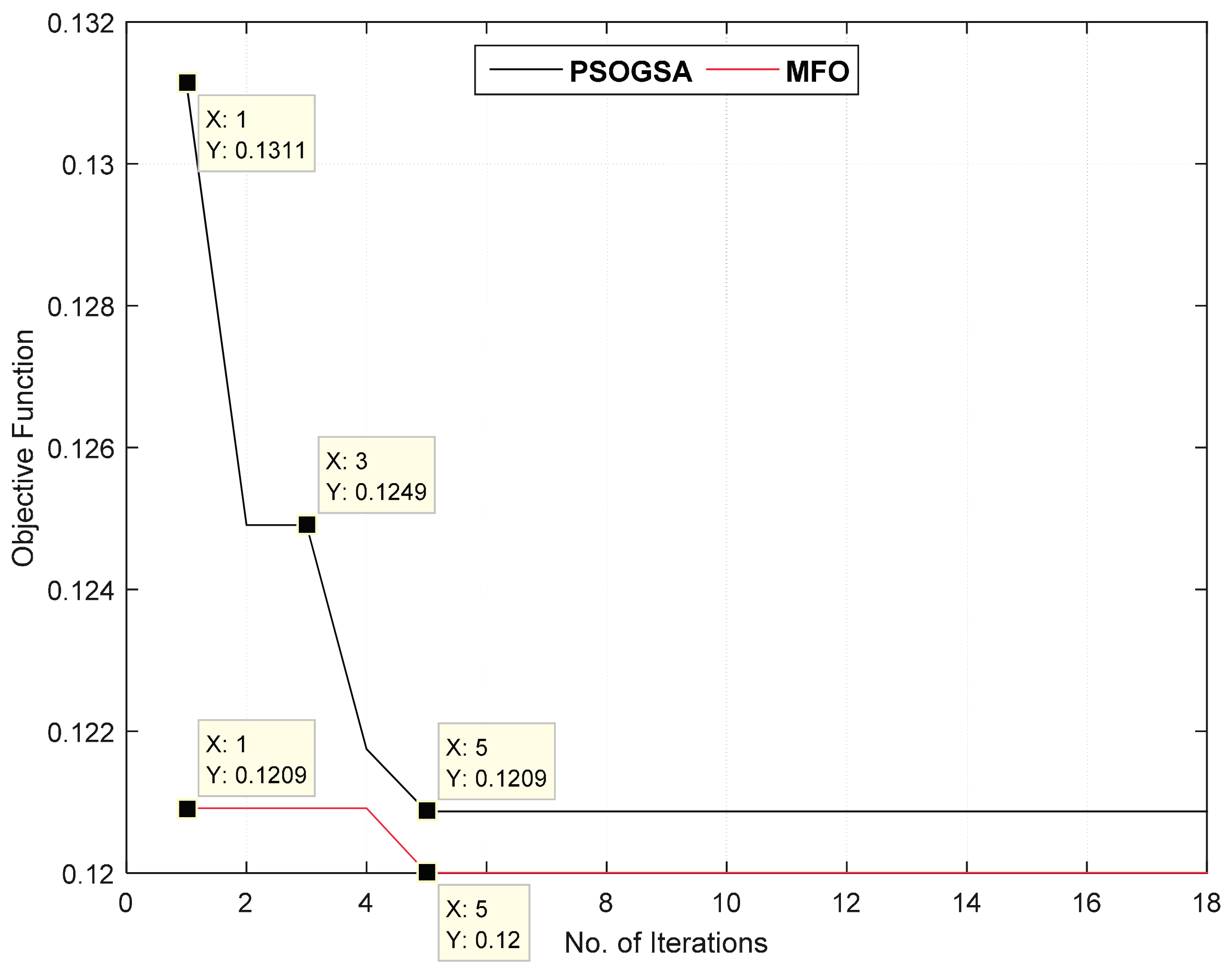
5.3. Statistical Evaluation of the PSOGSA and MFO Techniques

To evaluate and prove the performance of the PSOGSA and MFO techniques, it is required to define a set of metrics.

Table 8. Quality indexes employed for evaluating the performance of the proposed techniques.

Metric	Abbreviation	Formula
Relative error	RE	$\frac{{\displaystyle {\sum }_{i=1}^{n_r}(VLC{I}_i-VLC{I}_{\min })}}{VLC{I}_{\min }}\times 100\%$
Mean absolute error	MAE	$\frac{{\displaystyle {\sum }_{i=1}^{n_r}(VLC{I}_i-VLC{I}_{\min })}}{n_r}$
Root mean square error	RMSE	$\sqrt{\frac{{\displaystyle {\sum }_{i=1}^{n_r}(VLC{I}_i-VLC{I}_{\min })}}{n_r}}$
Standard deviation	SD	$\sqrt{\frac{{\displaystyle {\sum }_{i=1}^{n_r}(VLC{I}_i-\overline{VLCI})}}{n_r}}$
Efficiency	-	$\frac{VLC{I}_{\min }}{VLC{I}_i}\times 100\%$

has various quality metrics to evaluate the PSOGSA and MFO optimization algorithms. Such indexes include the Relative Error RE, Mean Absolute Error (MAE), Root Mean Square Error (RMSE), standard deviation (STD) and Median. These metrics measure the values of the best minimum value of objective function (LVCI_min) and the value of objective function at each time of run (LVCI_i) which is obtained by the optimization algorithm. In Table 8, (n_r) is the number of data-set groups (runs of the power system). The parameters of each algorithm are set as the original references of the number of iterations (20) and the size of population and the number of agents for both PSOGSA and MFO respectively are (30) for 33-bus and 69-bus IEEE grids.

Table 9. Performance evaluation of PSOQN and PSOGSA algorithms under different cases “Number of runs is 30”.

Power Factor	System	Best Minimum Value of Objective Function VLCIbest	Worst Value of Objective Function VLCIworst	Median	SD %	Average RE	MAE Mean Absolute Error	RMSE Root Mean Square Error	Efficiency %
At unity	33-bus PSOGSA	0.3006	0.3027	0.3027	0.0184	0.2018	0.0020	0.0020	99.3317
	33-bus MFO	0.3005	0.3006	0.3006	0.0060	0.0320	3.2000 × 10−4	3.2547 × 10−4	99.8935
At 0.866	33-bus PSOGSA	0.1623	0.1812	0.1653	0.4866	0.7695	0.0042	0.0063	97.5773
	33-bus MFO	0.1615	0.1616	0.1615	0.0288	0.1549	8.2888 × 10−4	8.7590 × 10−4	99.4865
At unity	69-bus PSOGSA	0.2635	0.2644	0.2644	0.0160	0.1062	7.1556 × 10−4	7.3260 × 10−4	99.6471
	69-bus MFO	0.2635	0.2642	0.2642	2.2584 × 10−14	0.0815	9.3320 × 10−4	9.3320 × 10−4	99.7292
At 0.866	69-bus PSOGSA	0.1200	0.1252	0.1209	0.1560	0.4282	0.0017	0.0023	98.6080
	69-bus MFO	0.1200	0.1240	0.1200	0.0726	0.0331	1.3259 × 10−4	7.2624 × 10−4	99.8931

Bold items represent the best performance evaluation results of MFO technique.

shows the performance evaluation of PSOGSA and MFO for two RDGs types. From this table, it is observed that MFO has acceptable RMSE. Moreover, the STD demonstrates that the results don’t change along the iterative process, which indicated the stability of the proposed MFO algorithm as compared with PSOGSA technique. According to the previous discussion, the MFO has the highest performance and accuracy to find the optimum RDGs allocation and capacity as compared as PSOGSA.

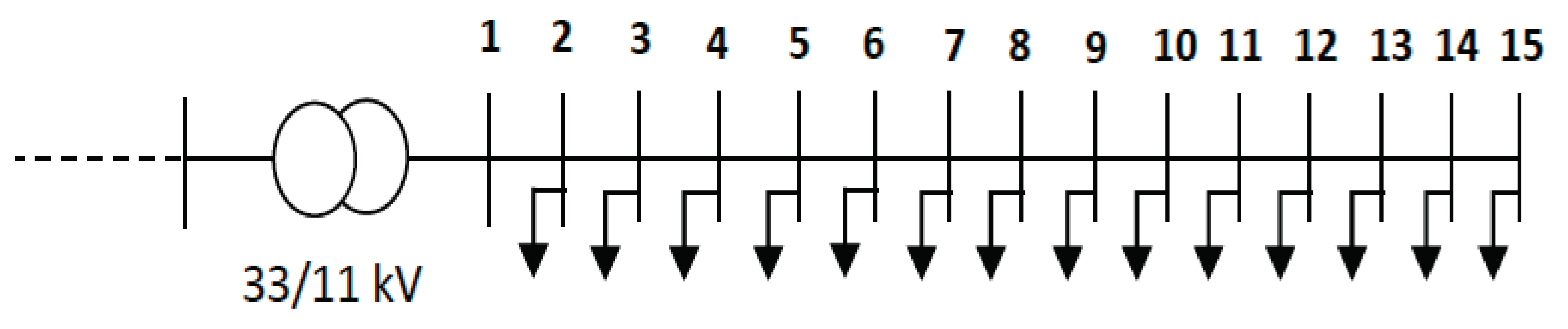
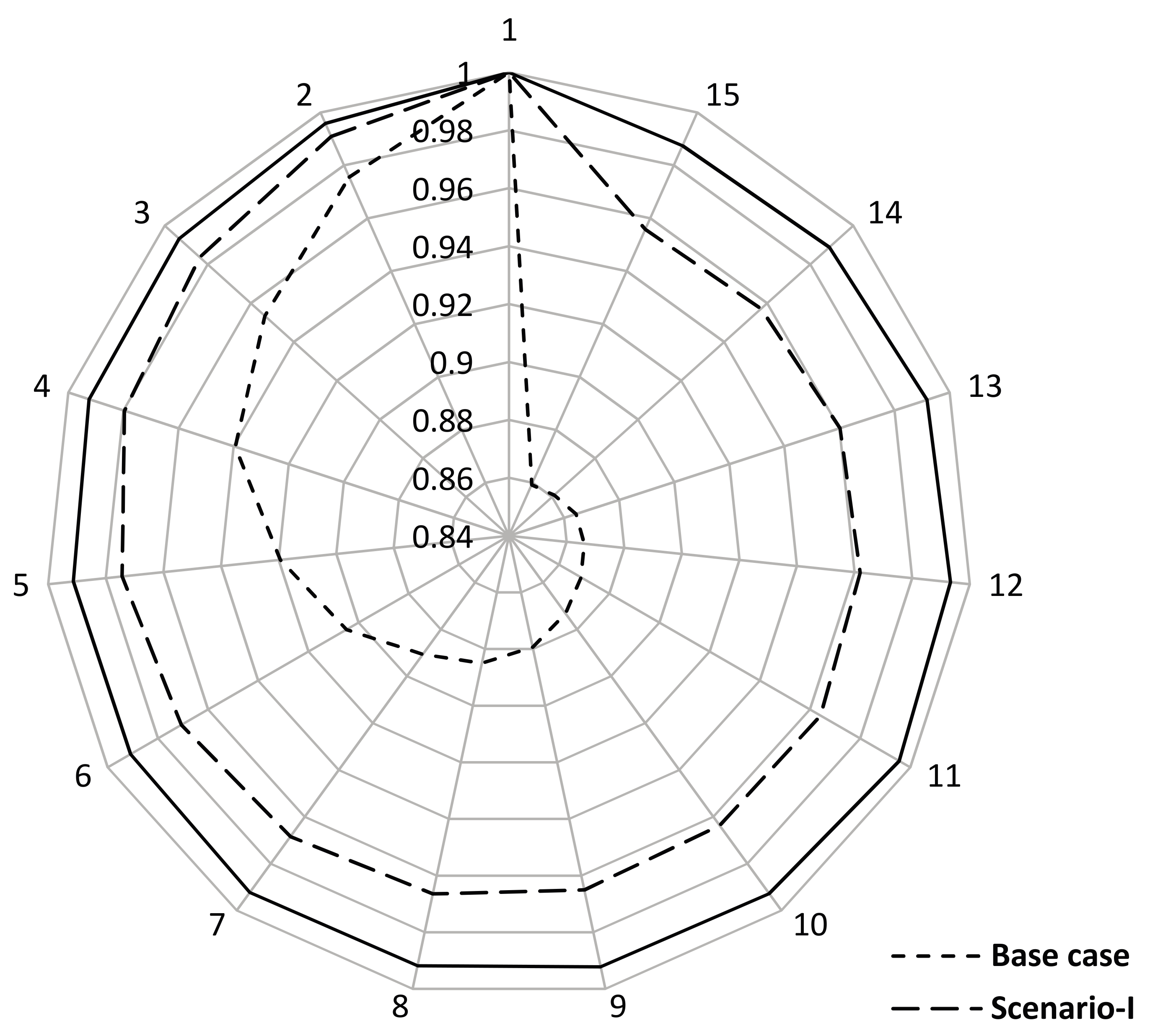
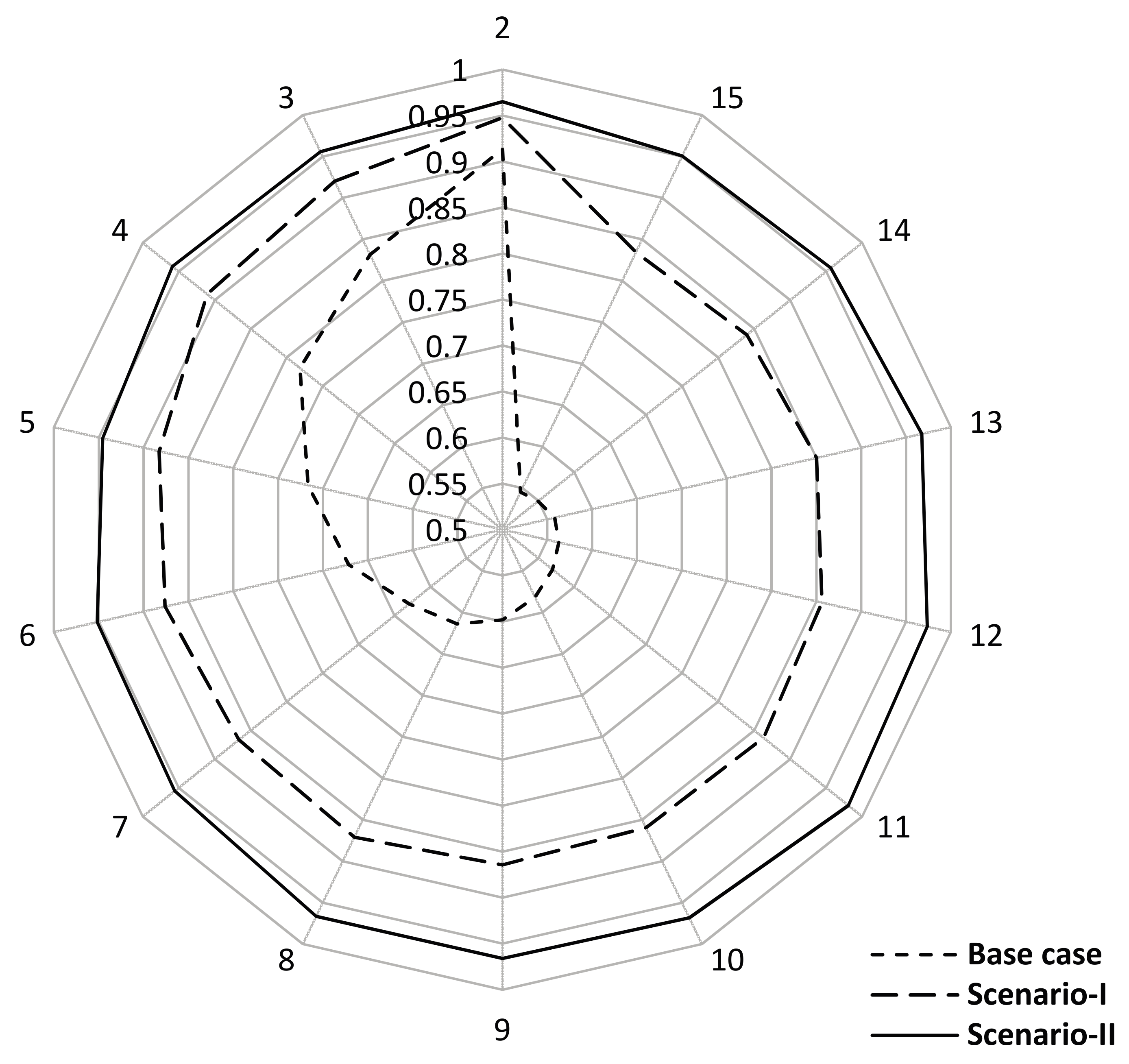
5.4. Egyptian Practicle Case Study Distribution Network

According to the previous comparisons between the MFO and PSOGSA techniques, the MFO proves its superiority with high attitude to determine the optimal placement and sitting of RDGs on distribution network, therefore the MFO is applied to the MEDN case study to solve its problems.

The Egyptian case study is studied at 14:00 h, because it is deemed as the maximum peak of load level. The system data of MEDN in our calculations and analysis are as follows; the base voltage of the MEDN at slack-bus-1 = 11 kV, the total system apparent power (S_total) = 2201.8 + j 1018.9 kVA, Apparent load power (S_load) = 1976.3 + j 865.2 kVA and Apparent loss power (S_loss) = 225.46 + j 153.67 kVA. The voltage magnitude limits are considered between 0.95 and 1.05 p.u. In this case study the maximum limit of total active power $P_{T,DG}^{\max }$ of RDGs that integrated on MEDN is suggested to be 85% from the total load of the system P_Load ($P_{T,DG}^{\max }=0.85\times P_{Load}$), to avoid the excess integration of active power to the network. Moreover, the increase in the maximum limit range of integrated active power into the network, by default, will increase the possibilities of finding the most optimum size of RDGs without any violation of constraints. Two scenarios are suggested to study the impacts of RDGs on the MEDN case study. In scenario-I, the PV system is integrated at unity PF only. Based on the LSF and VSF algorithms, the optimum candidate buses by MFO technique is 7 and 11 buses.

From

Table 10. The results of 15-bus of MEDN with PV and/or WT systems at maximum peak load (14:00 h).

Items	Base Case	Scenario-I		Scenario-II
Total losses (kW)	225.46	39.0044		7.9184
Loss reduction %	-	82.70		96.4878
Vmin (p.u.)/bus	0.8593/15	0.9558/15		0.9874/15
VSImin (p.u.)/bus	0.5453/15	0.8344/15		0.9457/5
Optimal location buses and size of RDGs (kW)	-	(7)	500	(7)	450
	-	(11)	1050	(11)	1050
SDG,T (kVA)	-	1550		1732.1
RDGs Power Factor (PF)	-	unity		0.866
TOC ($)	-	7906		7531.7
ΔVDev	-	0.0442		0.0126
ΔPlDG	-	0.1730		0.0351
ΔOC	-	0.9413		0.8967
Objective Function	-	0.1983		0.1123
Elapced time(s)	-	1.5		2.1

, the optimum capacities of PV system are (7) 500 kW and (11) 1050 kW. The total system losses is decreased to 82.7%. The V_min is improved from 0.8593 p.u. to 0.9558 p.u. in addition to the VSI_min is improved from 0.5453 to 0.8344. In Table 10, the optimum capacities of WT system are (7) 450 kW and (11) 1050 kW. The numerical results of scenario-II explain that the system power losses is minimized clearly to 96.49%, the V_min is increased to 0.9874 p.u., and the VSI_min is increased to 0.9457 p.u. In this regard, scenario-II with WT system at 0.866 PF has better results than scenario-I. The elapsed CPU time by MFO technique is calculated for PV system as 1.5 s and for WT system as 2.1 s. The impact of RDGs types on voltage profile level and voltage stability profile of MEDN is illustrated in Figure 26 and Figure 27. According to that, the MFO technique is efficient, faster and superior to deduce the optimal solutions of RDGs type’s allocations in MEDN case study.

6. Conclusions

In this article, a novel strategy based on hybrid PSOGSA and MFO techniques is proposed to find the optimal allocation and capacity of RDGs in different radial distribution networks. Appropriate sensitivity factors are produced to reduce the search space of both algorithms by estimating the most candidate buses for the RDG units’ allocation. For power flow calculations, the backward/forward sweep algorithm is applied. The proposed PSOGSA and MFO scheme has been tested on 33-bus and 69-bus IEEE grids. The results of the proposed algorithms have been compared with other methods to validate the approach. The results illustrate that the proposed MFO approach is very fast as compared with PSOGSA. Moreover, MFO has a high accuracy and performance to predict the optimum solutions. For example, in 33-bus at 0.866 PF (WT system), the MFO can find the optimum solutions in the 4th iteration within 9.3 s, but the PSOGSA reaches to the optimum solution in the 5th iteration within 10.2 s. Furthermore, with MFO technique, the system power loss is minimized to 86.153%, voltage profile and voltage stability are improved to 0.9803 p.u. and 0.9209 p.u., respectively, and the total operating cost (TOC) is minimized to 9366.9$. While, with PSOGSA, the system power loss is minimized to 86.013%, voltage profile and voltage stability are improved to 0.9798 p.u. and 0.9207 p.u., respectively, and the total operating cost (TOC) is minimized to 9368$. The average efficiency of MFO and PSOGSA based on the statistical evaluations are 99.75% and 99.04%, respectively. Therefore, it is clear that the proposed scheme MFO is capable of improving the voltage profile and voltage stability, minimizing the system losses and the total operating costs at multi RDGs types that are considered at different power factors as compared with PSOGSA and other techniques. According to the superiority of MFO and its capability to find the optimal solutions of RDGs, it is applied on MEDN to solve its drawbacks. The case study of MEDN is selected at the maximum peak load, which it is considered as the worst case. It is suggested two scenarios also. In scenario-I that includes PV system at unity PF, the MFO is decreased the system power losses to 82.7% and improved the voltage profile and voltage stability to 0.9558 p.u. and 0.8344 p.u. Thus, in scenario-II that includes WT system at 0.866 PF, the MFO is decreased the system power losses to 96.4878% and improved the voltage profile and voltage stability to 0.9874 p.u. and 0.9457 p.u. Therefore, the scenario-II has more impact on the MEDN system with better results as compared as scenario-I. As future work we plan to study and analyze the dynamic operation, voltage unbalances and stability of the network with RDGs during faults.

References

1. Ou, T.-C.; Hong, C.-M. Dynamic operation and control of microgrid hybrid power systems. Energy 2014, 66, 314–323. [Google Scholar] [CrossRef]
2. Ou, T.-C. A novel unsymmetrical faults analysis for microgrid distribution systems. Electr. Power Energy Compon. 2012, 43, 1017–1024. [Google Scholar] [CrossRef]
3. Ou, T.-C.; Lu, K.-H.; Huang, C.-J. Improvement of Transient Stability in a Hybrid Power Multi-System Using a Designed NIDC. Energies J. 2017, 10, 1–16. [Google Scholar]
4. Tulsky, V.; Vanin, A.; Tolba, M.; Sharova, A.; Diab, A. Study and analysis of power quality for an electric power distribution system—Case study: Moscow region. In Proceedings of the 2016 IEEE NW Russia Young Researchers in Electrical and Electronic Engineering Conference (EIConRusNW), St. Petersburg, Russia, 2–3 February 2016; pp. 710–716. [Google Scholar] [CrossRef]
5. Chiradeja, P.; Ramkumar, R. An Approach to Quantify the Technical Benefits of Distribute Generation. IEEE Trans. Energy Convers. 2004, 19, 764–773. [Google Scholar] [CrossRef]
6. Niknam, T. A new approach based on ant colony optimization for daily Volt/Var control in distribution networks considering distributed generators. Energy Convers. Manag. 2008, 49, 3417–3424. [Google Scholar] [CrossRef]
7. Abdelaziz, A.; Hegazy, Y.; El-Kattam, W.; Othman, M. Optimal Planning of Distributed Generators in Distribution Networks Using Modified Firefly Method. Electr. Power Compon. Syst. 2015, 43, 320–333. [Google Scholar] [CrossRef]
8. Gupta, S.; Saxena, A.; Soni, B.P. Optimal Placement Strategy of Distributed Generators based on Radial Basis Function Neural Network in Distribution Networks. Procedia Comput. Sci. 2015, 57, 249–257. [Google Scholar] [CrossRef]
9. Kalambe, S.; Aggnihotri, G. Loss minimization techniques used in distribution network: Bibliographical survey. Renew. Sustain. Energy Rev. J. 2014, 29, 184–200. [Google Scholar] [CrossRef]
10. Liu, W.; Xu, H.; Niu, S.; Jiang, X. Optimal Distributed Generator Allocation Method Considering Voltage Control Cost. Sustain. J. 2016, 8, 193. [Google Scholar] [CrossRef]
11. Reddy, V.V.; Manohar, T.G. Optimal renewable resources placement in distribution networks by combined power loss index and whale optimization algorithms. J. Electr. Syst. Inf. Technol. 2017. [Google Scholar] [CrossRef]
12. Sudabattula, S.; Kowsalwa, M. Optimal allocation of wind based distributed generators in distribution system using Cuckoo Search Algorithm. Procedia Comput. Sci. 2016, 92, 298–304. [Google Scholar] [CrossRef]
13. Georgilakis, P.; Hatziargyriou, N. Optimal distributed generation placement in power distribution networks: Models, methods and future research. IEEE Trans. Power Syst. 2013, 28, 3420–3428. [Google Scholar] [CrossRef]
14. Wang, H.; Huang, J. Cooperative planning of renewable generation for interconnected microgrids. IEEE Trans. Smart Grid 2016, 7, 2486–2496. [Google Scholar] [CrossRef]
15. Wang, H.; Huang, J. Joint investment and operation of microgrid. IEEE Trans. Smart Grid 2017, 8, 833–845. [Google Scholar] [CrossRef]
16. Liu, Y.; Tan, S.; Jiang, C. Interval optimal scheduling of hydro-PV-wind hybrid system considering firm generation coordination. IET Renew. Power Gener. 2017, 11, 63–72. [Google Scholar] [CrossRef]
17. El-Fergany, A. Optimal allocation of multi-type distributed generators using backtracking search optimization algorithm. Electr. Power Energy Syst. 2015, 64, 1197–1205. [Google Scholar] [CrossRef]
18. Singh, R.; Gowsami, S. Optimum allocation of distributed generations based on nodal pricing for profit, loss reduction, and voltage improvement including voltage rise issue. Electr. Power Energy Syst. 2010, 32, 637–644. [Google Scholar] [CrossRef]
19. Moradi, M.; Abedini, M. A combination of genetic algorithm and particle swarm optimization for optimal DG location and sizing in distribution systems. Electr. Power Energy Syst. 2012, 34, 66–74. [Google Scholar] [CrossRef]
20. Injeti, S.; Kumar, N. A Novel Approach to Identify Optimal Access Point and Capacity of Multiple DGs in a Small, Medium and Large Scale Radial Distribution Systems. Electr. Power Energy Syst. 2013, 45, 142–151. [Google Scholar] [CrossRef]
21. Imran, M.; Kowsalya, M. Optimal size and siting of multiple distribution generators in distribution system using bacterial foraging optimization. Swarm Evol. Comput. 2014, 15, 58–65. [Google Scholar] [CrossRef]
22. Shirmohammadi, D.; Hong, H.; Semlyen, A.; Lou, G. A compensation-Based Power Flow Method for Weakly Meshed Distribution and Transmission Networks. IEEE Trans. Power Syst. 1988, 3, 753–762. [Google Scholar] [CrossRef]
23. Injeti, S.; Thunuguntla, V.; Shareef, M. Optimal allocation of capacitor banks in radial distribution systems for minimization of real power loss and maximization of network savings using bio-inspired optimization algorithms. Electrical Power Energy Syst. 2015, 69, 441–455. [Google Scholar] [CrossRef]
24. Institute of Electrical and Electronics Engineers. IEEE Standard 1159-2009, IEEE Recommended Practice for Monitoring Electric Power Quality; Institute of Electrical and Electronics Engineers: Piscataway, NJ, USA, 2009. [Google Scholar]
25. Institute of Electrical and Electronics Engineers. IEEE Standard 1346-1998, IEEE Recommended Practice for Evaluation Electric Power System Compatibility with Electronic Process Equipment; Institute of Electrical and Electronics Engineers: Piscataway, NJ, USA, 1998. [Google Scholar]
26. International Electrotechnical Commission. IEC Standard 61000-4-30, Electromagnetic Compatibility (EMC)—Part 4-30: Testing and Measurement Techniques—Power Quality Measurement Methods; International Electrotechnical Commission: Geneva, Switzerland, 2015. [Google Scholar]
27. Awaise, A. Case study of flexible operations in Egypt. In Proceedings of the IAEA, Technical Meeting on Flexible (Non-Baseload) Operation for Load Following and Frequency Control in New NPP’s, Erlangen, Germany, 6–8 October 2014; Available online: https://www.iaea.org/NuclearPower/Meetings/2014/ (accessed on 20 December 2017).
28. Fetouh, T.; Kawady, T.; Shaaban, H.; Elsherif, A. Impact of the New Gabl El-Zite Wind Farm Addition on the Egyptian Power System Stability. In Proceedings of the 2013 13th International Conference on Environment and Electrical Engineering (EEEIC), Wroclaw, Poland, 1–3 November 2013. [Google Scholar]
29. Devabalaji, K.; Yuvaraj, T.; Ravi, K. An efficient method for solving the optimal sitting and sizing problem of capacitor banks based on cuckoo search algorithm. Ain Shams Eng. J. 2016, in press. [Google Scholar] [CrossRef]
30. Mirjalili, S.; Hashim, Z. A new Hybrid PSOGSA Algorithm for function optimization. In Proceedings of the 2010 International Conference on Computer and Information Application (ICCIA), Tianjin, China, 3–5 December 2010. [Google Scholar]
31. Eberhart, R.; Kennedy, J. A new optimizer using particles swarm theory. In Proceedings of the 6th International Symposium on Micro Machine and Human Science, Nagoya, Japan, 4–6 October 1995; pp. 39–43. [Google Scholar] [CrossRef]
32. Kennedy, J.; Eberhart, R. Particle swarm optimization. In Proceedings of the IEEE International Conference on Neural Networks IV, Perth, WA, Australia, 27 November–1 December 1995; pp. 1942–1948. [Google Scholar]
33. Rashedi, E.; Nezamabadi, S.; Saryazdi, S. GSA: A Gravitational Search Algorithm. Inf. Sci. 2009, 179, 2232–2248. [Google Scholar] [CrossRef]
34. Mirjalili, S. Moth-flame optimization algorithm: A novel nature-inspired heuristics paradigm. Knowl.-Based Syst. 2015, 89, 228–249. [Google Scholar] [CrossRef]
Figure 1. Egyptian Electrical Unified Network (EEUN).
Energies 11 00245 g001
Figure 2. The measured case study of the Middle Egypt Distribution Network (MEDN) at the nodes with black circle.
Energies 11 00245 g002
Figure 3. A case study 15-bus distribution network of MEDN.
Energies 11 00245 g003
Figure 4. Measurement of voltage profile in (kV) through 24 h.
Energies 11 00245 g004
Figure 5. Graph of active and reactive power loads at each bus at 11 kV within 24-h.
Energies 11 00245 g005
Figure 6. A sample of distribution network.
Energies 11 00245 g006
Figure 7. Flow chart of PSOGSA algorithm.
Energies 11 00245 g007
Figure 8. Spirally flying path around near light sources [34]. (Reproduced with permission by Elsevier publisher, 2018)
Energies 11 00245 g008
Figure 9. Temporary position that can be reached by a moth with regard to a flame using the logarithmic spiral [34]. (Reproduced with permission by Elsevier publisher, 2018).
Energies 11 00245 g009
Figure 10. Flow chart of MFO Algorithm.
Energies 11 00245 g010
Figure 11. The line diagram of IEEE 33-bus radial distribution network.
Energies 11 00245 g011
Figure 12. The change of objective function (LVCI) with iterations number for 33-bus at unity PF.
Energies 11 00245 g012
Figure 13. The change of objective function (LVCI) with iterations number for 33-bus at 0.866 PF.
Energies 11 00245 g013
Figure 14. The impact of compensated devices on voltage profile for 33-bus IEEE system at unity PF.
Energies 11 00245 g014
Figure 15. The impact of compensated devices on voltage profile for 33-bus IEEE system at 0.866 PF.
Energies 11 00245 g015
Figure 16. The impact of compensated devices on VSI profile for 33-bus IEEE system at unity PF.
Energies 11 00245 g016
Figure 17. The impact of compensated devices on VSI profile for 33-bus IEEE system at 0.866 PF.
Energies 11 00245 g017
Figure 18. Comparison of different performances for 33-bus system.
Energies 11 00245 g018
Figure 19. The schematic diagram of IEEE 69-bus radial distribution network.
Energies 11 00245 g019
Figure 20. The change of objective function (LVCI) with iterations number for 69-bus at unity PF.
Energies 11 00245 g020
Figure 21. The change of objective function (LVCI) with iterations number for 69-bus at 0.866 PF.
Energies 11 00245 g021
Figure 22. The impact of compensated devices on voltage profile for 69-bus IEEE system at unity PF.
Energies 11 00245 g022
Figure 23. The impact of compensated devices on voltage profile for 69-bus IEEE system at 0.866 PF.
Energies 11 00245 g023
Figure 24. The impact of compensated devices on VSI profile for 69-bus IEEE system at unity PF.
Energies 11 00245 g024
Figure 25. The impact of compensated devices on VSI profile for 69-bus IEEE system at 0.866 PF.
Energies 11 00245 g025
Figure 26. The impact of compensated devices on voltage profile for 15-bus of MEDN with PV and WT.
Energies 11 00245 g026
Figure 27. The impact of compensated devices on voltage stability profile for 15-bus of MEDN with PV and WT.
Energies 11 00245 g027