An Intelligent Fault Diagnosis Method for Bogie Bearings of Metro Vehicles Based on Weighted Improved D-S Evidence Theory

Abstract

Bogie bearings are very important for the safe and normal operation of metro vehicles. The prevailing fault diagnosis methods for bogie bearings generally utilize a single information source, such as vibration, temperature or acoustics. There are some shortcomings in these methods, including low accuracy and poor reliability. To address these shortcomings, this paper proposes an intelligent fault diagnosis method. Based on improved D-S (Dempster-Shafer) evidence theory, this method comprehensively analyzes vibration and temperature signals to diagnose bearing faults. In order to verify the feasibility and effectiveness of the proposed method, this study designed the hardware device and constructed a test platform. Bogie bearings with faults occurring on the outer ring, inner ring and rolling elements were tested on this platform. The diagnosis accuracy rate of the proposed fusion algorithm reached 91%, and the misdiagnosis rate was only 2%. The test results showed that the proposed method can accurately and reliably realize fault diagnosis with a high accuracy rate and a low misdiagnosis rate compared to previous methods. Thus, the proposed fault diagnosis method can accurately and effectively identify the faults of metro vehicle bogie bearings.

1. Introduction

With the rapid development of urban rail transit construction, masses of metro vehicles have been put into use, which attracts significant attention to the normal and safe operation of these metro vehicles. As a vital part of a metro vehicle system, the normal operation of bogie bearing system is important. Failures of the bearing system will endanger the normal operation of vehicles, or even cause accidents. Therefore, for traffic safety it is essential to detect and forecast failures before unnecessary loss occurs.

At present, most railway operation departments adopt a maintenance mechanism of regular inspection, which has limitations. Many experts and scholars have made efforts to develop more intelligent methods for fault diagnosis of bearings. Previous, fault diagnosis methods for rolling bearings mainly include acoustic based methods, temperature based methods, stray flux measurement based methods, vibration based method, etc. Frosini et al., and Henao et al. [1,2] introduced a bearing fault detection technology based on stray flux measurement technology. This method relies on the statistical processing of the measurements of this flux in different positions around the induction motor (IM). It is complicated to measure flux in different positions. Vibration based method is one of the most widely used method for fault diagnosis of rolling bearings, because vibration based fault characteristics are easy to detect online when a fault occurs in the bearings [3]. Research based on vibration signals can be classified into three categories. In the time domain [4], some parameters such as mean value, root-mean square, variance, kurtosis, etc., are extracted for fault diagnosis since they are always sensitive to the fault state. In the frequency domain, Fourier transform and its variations such as fast Fourier transform and short-time Fourier transform are used for analysis [5]. In the time-frequency domain, wavelet transform [6] and wavelet packet transform [7] are effective tools for time-frequency analysis, which have been widely utilized in fault diagnosis. Kankar et al., and Bin et al. [6,7] have introduced the application of wavelet transform and wavelet packet transform in the extraction of fault characteristics for rolling bearing fault diagnosis, and proved that wavelet transform and wavelet packet transform are effective in extracting fault characteristics.

Most of the early intelligent diagnosis methods are based on single source information, which are unreliable and unsafe to some extent. Multi-source information diagnosis methods for bearings have been highly researched in recent years, and mainly include Fuzzy Sets theory, Neural Networks and D-S evidence theory (Dempster-Shafer evidence theory). First proposed by L.A. Zadeh, Fuzzy Sets theory [8] has been studied and used in fault diagnosis. For example, Xia and Chen [9] have studied the evolutionary process of a fault bearing performance and have proposed a diagnosis method based on Fuzzy Sets theory; the proposed method has achieved good results. However, the Fuzzy Sets theory has a significant defect because it lacks a unified, scientific theoretical basis, thus, the findings in one field may not be easily used in another field. Recently, Neural Networks has also been widely studied in the diagnosis field [10,11]. By establishing mapping from analog signals to digits 0 and 1, Neural Networks can approximate any nonlinear continuous function with arbitrary precision. Nevertheless, almost all the studies have found that it is difficult for people to generalize the established network. It needs a large number of samples to train the network, and even the established network may break down if the inputs are inadequate. What is more, there is a common flaw in these two theories, that is, they cannot explain the calculation process clearly. The shortcomings referred to above restrict the application of Fuzzy Sets theory and Neural Networks.

D-S evidence theory has become the focus of recent study. By establishing the frame of discernment and assigning mass functions, D-S evidence theory provides a way to deal with uncertain and imprecise information, which is the reason it is very suitable for fault diagnosis [12]. Compared with Fuzzy Sets theory and Neural Networks, the presentation of D-S evidence theory is specific and the calculation process is obvious. Besides, D-S evidence theory is easy to execute and generalize. So, given these attributes, D-S evidence theory is superior to the other two methods. However, when facing a situation where evidence highly conflicts, the classic D-S evidence theory appears to be imperfect as the fusion results may be counter-intuitive. In this respect, many scholars have been working on improving classic D-S evidence theory [13,14]. The improved methods can be divided into two categories: methods based on the processing of mass functions and methods based on the modification of fusion rules [15,16,17]. In this paper, an intelligent fault diagnosis method for metro vehicle bogie bearings based on a weighted improved D-S evidence theory is proposed. This method modifies the fusion rules as well as weighting the original evidence. Three fault characteristics, including peak–peak ratio (P) at fault characteristic frequency of envelope spectrum, kurtosis factor (K_v) of vibration signal in the time domain and temperature signal, are extracted for comprehensive analysis. In order to test the proposed intelligent diagnosis method, a hardware device was designed and a bearing fault diagnosis test platform was constructed. The test results show that the proposed fault diagnosis method can effectively identify the bearing faults.

This paper is organized as follows: the second section introduces basic theories, including D-S evidence theory, wavelet packet transform and Hilbert transform; the third section derives the improved D-S evidence fusion algorithm; the fourth section builds the bearing fault diagnosis model based on the improved D-S evidence fusion algorithm proposed in the third section; the fifth and sixth section verify the effectiveness of the proposed intelligent fault diagnosis method for bogie bearings by experiment results; and the seventh section concludes this paper.

2. Introduction of Basic Theories

2.1. D-S Evidence Theory

Multi-source information fusion theory is derived from the need to comprehensively utilize multi-information for accurate results. D-S evidence theory has obvious advantages in dealing with uncertain information that is obtained from multiple sources, such as multiple sensors, different experts’ opinions, etc. It can still work even when there is a loss of information. Besides, D-S evidence theory takes into account the conflict between all information sources and even the conflict between one evidence source and another, so we can easily find out if the evidence is a defective value. In addition, D-S evidence theory is easily accessible and generalizable. Many scientific works have shown the wide applications of D-S evidence theory [18,19,20,21], such as remote sensing, the natural environment, human posture recognition, maintenance of power grid and power equipment, etc.

Let $\Theta :\{{\theta }_1,{\theta }_2,\dots ,{\theta }_N\}$ represent the frame of discernment, which is the finite set of N mutually exclusive elements ${\theta }_i(i=1,2,\dots N)$. All the possible subsets (focal elements) are called power sets denoted by $2^{\Theta }$. For example, if $\Theta :\{A,B,C\}$, then $2^{\Theta }=\left\{\phi ,\left\{A\right\},\left\{B\right\},\left\{C\right\},\{A,B\},\{A,C\},\{B,C\},\Theta \right\}$, where $\varphi$ means empty set. Define function $m:2^{\Theta }\to [0,1]$, and it satisfies the conditions:

$$\{\begin{array}{c}m(\varphi )=0\\ {\displaystyle \sum _{A\subseteq \Theta }m(A)=1}\end{array}$$

(1)

where A denotes non-empty focal element of power sets. m(A) reflects the belief measure for focal element A, which is called the basic probability assignment function or mass function. Also, D-S evidence theory defines two functions; namely, the belief function (Bel) and the plausibility function (Pls) to express uncertainty [22]. These two functions are both deduced from mass function.

$$\{\begin{array}{c}Bel(\varphi )=0\\ Bel(A)={\displaystyle \sum _{B\subseteq A}m(B),A\in 2^{\Theta },A\ne \varphi }\end{array}$$

(2)

$$\{\begin{array}{c}Pls(\varphi )=0\\ Pls(A)={\displaystyle \sum _{B\cap A=\varphi }m(B),A\in 2^{\Theta },A\ne \varphi }\end{array}$$

(3)

$Bel(A)$ is the sum of the probability of all the subsets of A, $Pls(A)$ is the sum of the probability of B which has no intersection with A. That is to say, $Bel(A)$ and $Pls(A)$ can be referred as the lower bound and upper bound of the belief for focal element A. So $\left[Bel(A),Pls(A)\right]$, which is called the belief interval, is used to express the uncertainty of A.

Supposing $m_1,m_2$ are two mass functions obtained from two evidence sources in the same frame of discernment, the fusion algorithm of the classic D-S evidence theory is:

$$m_{12}(C_l)=\{\begin{array}{cc}\frac{{\displaystyle \sum _{A_i\cap B_j=C_l}{m}_1(A_i)m_2(B_j)}}{1-K}& C_l\ne \varphi ,C_l\subset U\\ 0& C_l=\varphi \end{array}$$

(4)

$$K={\displaystyle \sum _{A_i\cap B_j=\varphi }{m}_1(A_i)m_2(B_j)}$$

(5)

where $A,B,C\subset U$ are focal elements.

2.2. Wavelet Packet Transform

Derived from wavelet transform, wavelet packet transform is an important tool for time-frequency analysis. It can decompose both the low frequency part and high frequency part of the signal. The wavelet packet decomposition algorithm is:

$$\{\begin{array}{c}{d}_{i,j,2m}={\displaystyle \sum _{k}h(k-2i)}{d}_{k,j+1,m}\\ d_{i,j,2m+1}={\displaystyle \sum _{k}g(k-2i)}{d}_{k,j+1,m}\end{array}$$

(6)

The wavelet packet reconstruction algorithm is:

$$d_{i,j+1,m}={\displaystyle \sum _{k}h(i-2k)}{d}_{k,j,2m}+{\displaystyle \sum _{k}g(i-2k)}{d}_{k,j,2m+1}$$

(7)

where d_i,j,m is the ith wavelet packet decomposition coefficient of the mth node in the jth layer.

The process of wavelet packet decomposition of three-layers is shown in Figure 1. S represents the original signal while A represents the low frequency part of the signal and D represents the high frequency part. The original signal can be divided into 8 bands, so we can analyze any one.

2.3. Hilbert Transform

Hilbert transform is a commonly used method for envelope analysis. Assuming that the Hilbert transform of a signal g(t) is ĝ(t), its mathematical expression is:

$$\stackrel{\wedge }{g}(t)=\frac{1}{\pi }{\displaystyle {\int }_{-\infty }^{+\infty }\frac{g(\tau )}{t-\tau }{d}_{\tau }}$$

(8)

Analytical signals can be generated based on the Hilbert transform with the original signal g(t) and its Hilbert transform ĝ(t), being the real part and the imaginary part of the analytical signal, respectively. That is,

$$g_{+}(t)=g(t)+j\stackrel{\wedge }{g}(t)$$

(9)

represented as the plural form is:

$$g_{+}(t)=A(t)e^{j\phi (t)}$$

(10)

In the formula,

$$A(t)=\sqrt{g^2(t)+\stackrel{\wedge }{g^2}(t)}$$

(11)

amplitude, $A(t)$ is the envelope of the signal $g(t)$.

If we process the envelope signal with FFT, the envelope spectrum of the signal can be obtained.

3. The Improved Evidence Fusion Algorithm

In the basic D-S evidence theory fusion algorithm, K is the normalization factor, which is a measure of conflict between all the evidence sources. If K is relatively small, the conflict between evidence sources is slight, that is, the belief trends of different evidence sources are similar, and the fusion results tend to assign more belief for the focal element of common trust. This effect of D-S evidence theory is called “focus”. However, if K is relatively large or K is close to 1, the conflict between evidence sources is very strong, that is, the belief trends of the evidence sources are sharply different. In this situation, the fusion result may be counter-intuitive.

To illustrate the shortcomings of the classic D-S evidence theory fusion rules, we assume:

(1)

The 2^Θ has three elements A, B, C and they have no intersection.

(2)

The mass functions obtained from two information sources are m₁, m₂.

According to (5), the conflict between evidence sources is:

$$\begin{array}{l}K={\displaystyle \sum _{A_i\cap B_j=\varphi }{m}_1(A_i)m_2(B_j)}\\ =m_1(A)m_2(B)+m_1(A)m_2(C)+m_1(B)m_2(A)+m_1(B)m_2(C)+m_1(C)m_2(A)+m_1(C)m_2(B)\end{array}$$

(12)

The sum of the basic probability distribution functions and the sum of trust of the synthetic results are 1. For the convenience of description, let

$$m{\prime }_{12}^{}(A)=m_1(A)m_2(A)$$

(13)

$$m{\prime }_{12}^{}(B)=m_1(B)m_2(B)$$

(14)

$$m{\prime }_{12}^{}(C)=m_1(C)m_2(C)$$

(15)

The conflict between evidence sources can also be expressed as:

$$K=1-{(m\prime }_{12}^{}(A)+m{\prime }_{12}^{}(B)+m{\prime }_{12}^{}(C))$$

(16)

The unfolded fusion rules of the classic D-S evidence theory can be expressed as:

$$m_{12}(A)=\frac{m_1(A)m_2(A)}{1-K}=m{\prime }_{12}^{}(A)+\frac{m{\prime }_{12}^{}(A)}{m{\prime }_{12}^{}(A)+m{\prime }_{12}^{}(B)+m{\prime }_{12}^{}(C)}\cdot K$$

(17)

$$m_{12}(B)=m{\prime }_{12}^{}(B)+\frac{m{\prime }_{12}^{}(B)}{m{\prime }_{12}^{}(A)+m{\prime }_{12}^{}(B)+m{\prime }_{12}^{}(C)}\cdot K$$

(18)

$$m_{12}(C)=m{\prime }_{12}^{}(C)+\frac{m{\prime }_{12}^{}(C)}{m{\prime }_{12}^{}(A)+m{\prime }_{12}^{}(B)+m{\prime }_{12}^{}(C)}\cdot K$$

(19)

where m’₁₂(x), (x = A, B, C) is the numerator in (4). From the unfolded fusion rules, we find that the reason why the classic D-S evidence theory tends to be wrong when dealing with high conflict evidence is that the conflict probability K is distributed to a focal element A, according to the result of m’₁₂(A)/(m’₁₂(A) + m’₁₂(B) + m’₁₂(C)). When the evidence sources have high conflict, for example, m₁(A) = 0.95, m₁(B) = 0.05, m₁(C) = 0, m₂(A) = 0, m₂(B) = 0.95, m₂(C) = 0.05, the conflict K = 0.9975, the fusion result is m₁₂(A) = 0, m₁₂(B) = 1, m₁₂(C) = 0, because the numerator m’₁₂(A) = 0, m’₁₂(C) = 0. Although the two mass functions show that B is not that believable, the fusion result believes B totally. This is unreasonable. Therefore, an improved fusion algorithm; the quadratic sum percentage conflict distribution fusion algorithm (QPCDA) is proposed based on the classic D-S evidence theory to resolve this issue. QPCDA distributes the conflict probability K to a focal element according to the percentage of the quadratic sum of the mass functions on the specific focal element rather than the product of mass functions. The formula is:

$$m_{12}(C_l)=\{\begin{array}{cc}\frac{{\displaystyle \sum _{A_i\cap B_j=C_l}{m}_1(A_i)m_2(B_j)}}{1-K}(1-K)+a_l\cdot K& C_l\ne \varphi ,C_l\subset U\\ 0& C_l=\varphi \end{array}$$

(20)

The coefficient of (1 − K) is the synthetic formula of the classical D-S evidence theory, a_l is called the distribution coefficient of conflict which is used to weight and distribute conflict probability, it is defined as:

$$a_l=\frac{{\displaystyle \sum _{A_i\cap B_j=C_l}(m_1{}^2(A_i)+m_2{}^2(B_j)})}{{\displaystyle \sum _{A_i\cap B_j=U}(m_1{}^2(A_i)+m_2{}^2(B_j))}}$$

(21)

Formula (20) can be simplified to (22):

$$m_{12}(C_l)=\{\begin{array}{cc}{\displaystyle \sum _{A_i\cap B_j=C_l}{m}_1(A_i)m_2(B_j)}+a_l\cdot K& C_l\ne \varphi ,C_l\subset U\\ 0& C_l=\varphi \end{array}$$

(22)

The main difference between QPCDA and classic D-S evidence theory is the calculation of coefficient a_l. If K is small, the fusion result is close to the result of the classic D-S evidence theory, because the result of (22) is determined mainly by the first-half part. However, under the condition of high conflict, K is large or even close to 1, the result of (22) is determined mainly by the second-half part, which avoids the unreasonable fusion result that appears in the classic D-S evidence theory fusion algorithm shown in (4). The normalized fusion result of the same example referred to above based on QPCDA is m₁₂(A) = 0.4994, m₁₂(B) = 0.0002, m₁₂(C) = 0.4994, which is much more reasonable.

In addition, classic D-S evidence theory believes all evidence sources equally while actually this is not always the case. For example, the reliability of evidence is not the same when we take the differences in sensor type, sensor precision, etc., into consideration. Therefore, a weighted quadratic sum percentage conflict distribution fusion algorithm (WQPCDA) is proposed. There is a basic principle for weighting so that the original properties of the evidence sources are not destroyed. Suppose the two weight coefficients are ω₁, ω₂, which satisfy ω₁ + ω₂ = 1. The higher the reliability of the evidence source is, the bigger the weight coefficient should be. The average support level of 2 evidence sources can be defined as:

$$\overline{m}={\displaystyle \sum _{i=1}^2{\omega }_i{m}_i}$$

(23)

Based on the principle of constant $\overline{m}$, the two weighted mass functions are:

$$m_1\prime =m_1$$

(24)

$$m_2\prime =2\cdot \overline{m}-m_1\prime$$

(25)

Then, the fusion algorithm of WQPCDA can be expressed as:

$$m{\prime }_{12}(C_l)=\{\begin{array}{cc}{\displaystyle \sum _{A_i\cap B_j=C_l}{m}_1\prime (A_i)m_2\prime (B_j)}+a_l\prime \cdot K\prime & C_l\ne \varphi ,C_l\subset U\\ 0& C_l=\varphi \end{array}$$

(26)

4. The Bearing Fault Diagnosis Model Based on Weighted Quadratic Sum Percentage Conflict Distribution Fusion Algorithm

4.1. The Frame of Discernment

The frame of discernment is the range of decision for fusion. For a bearing fault diagnosis system, the frame of discernment can be defined as H: {fault,uncertain,normal}. Where “uncertain” is the state between “fault” and “normal”.

4.2. Evidence Sources

When the rolling bearing with a local failure is in the process of operation, the fault point periodically hits other parts, generating cyclical impact. The impact is reflected in vibration and shaft temperature signals. Thus, vibration signal and shaft temperature signal are chosen as two basic information sources.

In terms of vibration signal, the time domain parameter is very sensitive to the impact of bearing faults [23]. Generally, time domain parameters include parameters with dimension and parameters without dimension. Though all the time domain parameters change when a fault occurs, the parameters with dimensions such as mean and root-mean squares are easily influenced by speed, load, etc. The parameters without dimension are stable and strong enough. Among the numerous parameters without dimension (such as the kurtosis factor, peak factor, and waveform factor), the kurtosis factor is very sensitive to periodic impulse signal. So, the kurtosis factor is particularly suitable for fault diagnosis of bearings because when a local fault occurs, there will be periodic impulses in the vibration signal. For this reason, we chose the kurtosis factor as one of the evidence sources. Its definition is:

$$K_v=\frac{{\displaystyle \sum _{i=1}^N{x}_i{}^4}}{N\cdot x_{rms}^4}$$

(27)

where x_rms is the root-mean square value of the signal. N is the number of sample points. If the bearing is running normally, the kurtosis factor is close to 3, conversely, the parameter is bigger than 3. The bigger the kurtosis factor is, the bigger the probability of fault is.

While the time domain parameter has the advantage of being sensitive to bearing faults, it cannot distinguish the fault type. The envelope parameter in the frequency domain can compensate for this defect because it has a one-to-one correspondence with fault type. When a local fault occurs, there will be peaks at specific frequency as well as its harmonic frequency; the specific frequency is called “fault characteristic frequency”. The calculation of theoretical fault characteristic frequency may be influenced by machine accuracy and mechanical wear. So, it is acceptable if the actual frequency value of the peak has a minor deviation from the theoretical fault characteristic frequency value. Different fault types of the bearing show different fault characteristic frequencies. The fault characteristic frequency of the outer ring of a bogie bearing is:

$$f_o=\frac{z}{2}(1-\frac{d}{D}\cos \alpha )f_r$$

(28)

The fault characteristic frequency of the inner ring of a bogie bearing is:

$$f_i=\frac{z}{2}(1+\frac{d}{D}\cos \alpha )f_r$$

(29)

The fault characteristic frequency of the rolling element of a bogie bearing is:

$$f_b=\frac{D}{2d}(1-\frac{d^2}{D^2}{\cos }^2\alpha )f_r$$

(30)

In (28)–(30), $d$ is the rolling element diameter, D is the bearing pitch diameter, α is the contact angle, and f_r is the rotating frequency of inner ring. The fault characteristic frequency can be used to identify the fault type.

We define a parameter, peak–peak ratio (P) to represent the probability of fault. To obtain this parameter, we take advantage of the time-frequency analysis tools. Firstly, the original vibration signal is decomposed into 8 frequency bands without omission and overlap by three-layer wavelet packet decomposition. Then, the decomposed wavelet packet coefficients are reconstructed by the reconstruction algorithm. Secondly, the envelope spectrum of the reconstructed signal in each frequency band is obtained by Hilbert transform and fast Fourier transform (FFT). Finally, the peak–peak ratio at the fault characteristic frequency in each envelope spectrum can be obtained by using the search algorithm [24]. The presentation of peak–peak ratio is:

$$P=\frac{x_{peak}}{x{\prime }_{peak}}$$

(31)

where x_peak is the maximum magnitude of the envelope spectrum at fault characteristic frequency, and x’_peak is the second maximum magnitude of the envelope spectrum in the search bandwidth range (the search bandwidth range is set to be 10 Hz and the middle frequency of the search bandwidth range is the fault characteristic frequency). The bigger the peak–peak ratio is, the bigger the probability of fault is. P is associated with the fault characteristic frequency, by which we can identify the fault type. So we choose the peak–peak ratio as a parameter for fault diagnosis.

When a fault occurs, the shaft temperature of the bearing appears to rise abnormally. So, we chose temperature variation over 1 min ($\Delta T$) as the third parameter.

To summarize, peak–peak ratio (E₁), the kurtosis factor (E₂) and temperature variation over 1 min (E₃) were chosen as the three evidence sources for diagnosis.

4.3. Mass Function

Mass functions are the basic unit of evidence fusion. Actually, there is no uniform algorithm to generate mass functions at present. In this paper, we adopt an algorithm based on Manhattan distance to generate the mass functions we need. The standard values of the three evidence sources are determined by theoretic derivation and experimental analysis. The standard values of the evidence sources in our test are shown in

Table 1. The standard values of evidence sources.

Standard Value (${\mathit{h}}_{\mathit{i}}$)	Fault	Uncertain	Normal
Peak-peak ratio ($E_1$)	1.8	1.5	1.2
Kurtosis factor ($E_2$)	4.0	3.5	3.0
Temperature variation ($E_3$)	4.0	1.5	0.2

.

For evidence source E_i, the standard values corresponding to the frame of discernment, H:{fault,uncertain,normal}, are h_ifau, h_iunc, h_inor respectively, which forms a standard vector h_i = [h_ifau,h_iunc,h_inor] (i is the serial number of the evidence source). Suppose the value of the extracted parameter is h_ix, then the Manhattan distance between extracted value and standard value is:

$$c_{ij}=|h_{ix}-h_{ij}|$$

(32)

where the h_ij represents the jth element of the standard vector corresponding to the ith evidence source. The smaller c_ij is, the closer the two values are. Correspondingly, the probability assignment for jth element of the mass function obtained from ith evidence source should be bigger. So, the jth element of the ith mass function can be defined as:

$$m_{ij}=\frac{1}{c_{ij}+\epsilon }$$

(33)

where ε is an adjustable parameter which can be determined according to the actual condition. ε is necessary because if the extracted value is very close to the standard value, namely, c_ij→0, 1/c_ij→∞, then the mass function m_ij tends to be senseless. Considering the sum of the three values of the mass functions in (33) may not be 1, normalization is necessary.

However, when it satisfies the formula: h_ix1 − h_ij = h_ij − h_ix2, the two values of c_ij are the same because c_ij is an expression of absolute value with symmetry. This is unwanted. So, when h_ix > h_io, where h_io represents the standard value of the fault state, a linear function $y=A+B\cdot x$ is adopted to fit m_io, approximately. Also, the other two mass functions (“uncertain”, “normal”) are assigned according to the following Formula (34),

$$\{\begin{array}{c}{m}_{i0}=A+B\cdot c_{i0}\\ m_{i1}=(1-m_{i0})\cdot c_{i1}/(c_{i1}+c_{i2})\\ m_{ij}=(1-m_{i0})\cdot c_{i2}/(c_{i1}+c_{i2})\end{array}$$

(34)

where A and B are coefficients determined by actual conditions.

4.4. The Bearing Fault Diagnosis Method Based on Weighted Quadratic Sum Percentage Conflict Distribution Fusion Algorithm

The flow diagram of the proposed bearing fault diagnosis method is shown in Figure 2.

(1)

Initialize: Let S = 0, U = 0, V = 0, V_redy = 0, T_redy = 0. S = 0, U = 0 and V = 0 represent the outer ring, inner ring and rolling element as fault free, otherwise a fault in the corresponding component is indicated. V_redy = 0 represents that the processing of vibration signal is in progress while T_redy = 0 reflects that the processing of the temperature signal is in progress, otherwise the corresponding progress is over.

(2)

Temperature is collected for the first time. If the collected temperature T₀ is bigger than the set threshold temperature, that means there is a serious fault in the bearing and measures must be taken immediately. According to the product quality supervision and inspection rules of the Chinese Ministry of Railways, there must be an alarm if the temperature of bearings exceeds 90 °C. So T_threshold is set to be 90 °C in this paper.

(3)

If the shaft temperature is smaller than the set threshold temperature, it starts the timer and starts to collect vibration signals and extract time domain parameters and envelope spectrum parameters. Then, the mass functions m₁, m₂ are fused by using the proposed fusion algorithm ($m_v=m_1\oplus m_2$). Set V_redy to 1. When time is up, we collect the shaft temperature for the second time and calculate the temperature variation in unit time (∆T), with which we generate the mass function m₃. When this is finished, set T_redy to 1.

(4)

If V_redy = 1 and T_redy = 1, we distribute the weight coefficients of m_v and m₃. Due to the fault of the bearings used in the experiment being relatively slight, there will not be an obvious change in temperature. That is, the vibration signal is more reliable for diagnosis than the temperature signal in our test conditions. For this reason, the weight coefficient of temperature should be relatively small. After numerous experiments, we set the weight coefficients of m_v and m₃ to be 0.7 and 0.3, respectively, under the rules of high sensitivity and low error rate.

(5)

Decision: If the fusion result m = {m_fau, m_unc, m_nor} satisfies the decision rules, there is a fault in the bearing. Set the corresponding fault flag variable S, U or V to 1. The decision rules are shown as follows:

a

m_fau > m_unc and m_fau > m_nor

b

m_fau − m_unc > δ and m_fau − m_nor > δ

where $\delta$ is the decision threshold, which is set according to the actual conditions. The bigger $\delta$ is, the higher the diagnosis precision is. In this paper, $\delta$ is set to be 0.3 according to numerous experiments in our constructed test platform.

5. Experimental Study

5.1 Bearing Fault Test Platform

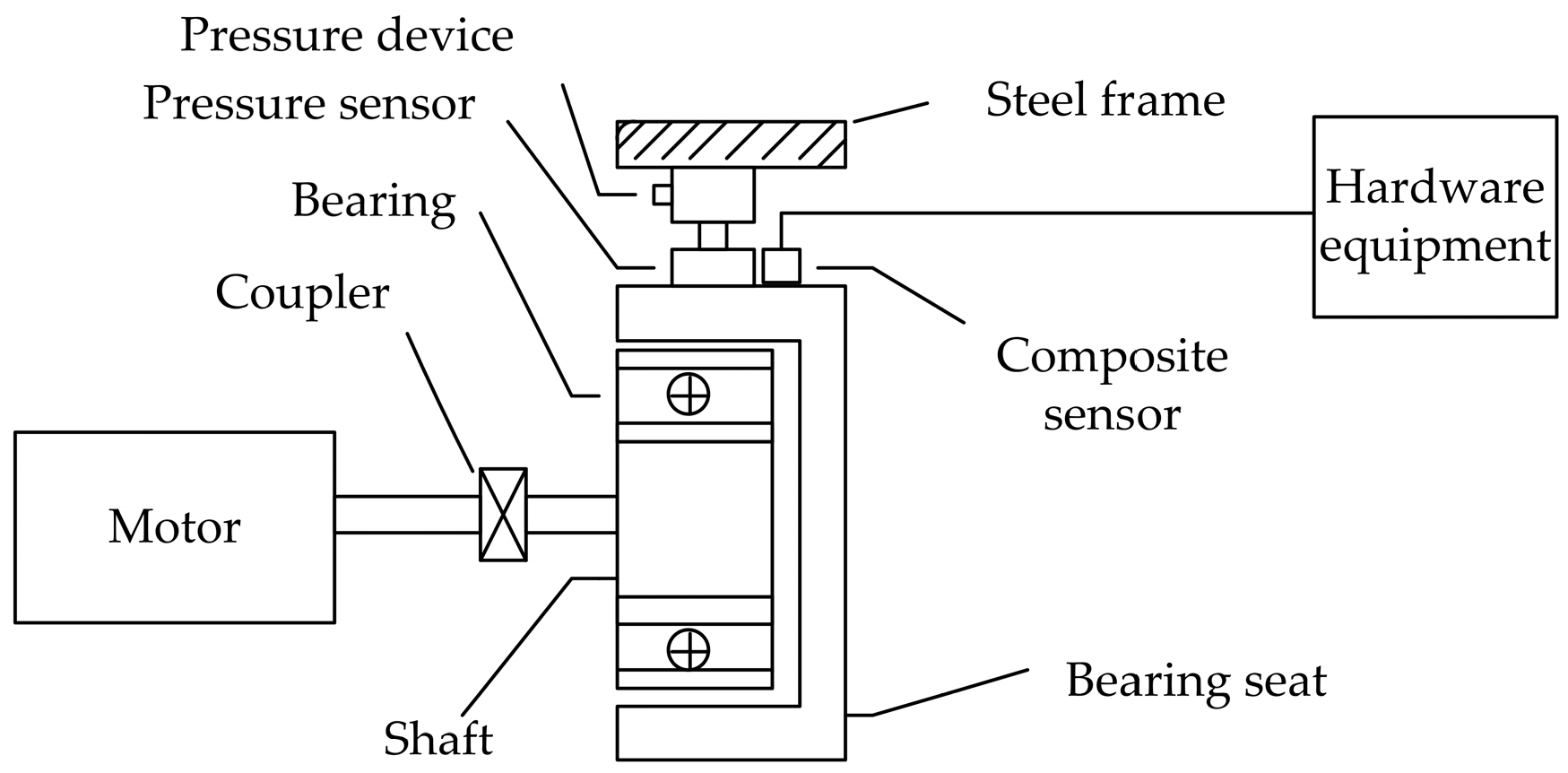
In order to verify the proposed fault diagnosis method, a test platform was constructed. The principle diagram of the platform is shown in Figure 3.

The motor drives the bearing inner ring to rotate. When it is running, the bearing produces vibration and temperature, which will be passed to the bearing seat. The acceleration sensor fixed on the bearing seat picks up the signals. The signals are collected and analyzed by the designed hardware to determine the bearing fault condition.

In the experiment, bearings with different kinds of faults were tested alternately. In order to facilitate loading and unloading of bearings, the bearing seat is designed into two parts, which are fixed together with the screws. A coupler is used since the size of the inner ring is different from the motor shaft. In order to simulate the influence of loads on the bearing operation, a steel frame is designed over the bearing seat. A pressure device (jack) is put between the steel frame and the bearing seat to generate radial pressure on the bearing seat, which simulates the vehicle load. In addition, a pressure sensor is placed in the middle of the bearing seat to measure the value of the pressure. The bearing seat and the steel frame are fixed on iron benches on the ground by screws.

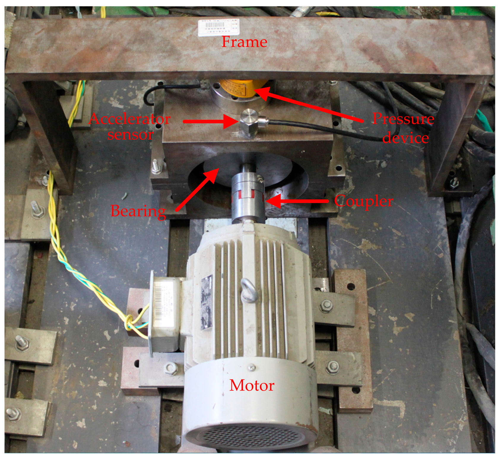
Figure 4 shows the physical test platform. A Siemens motor 1LG0106-4AA20 (Siemens Motor Co., Ltd., Jiangsu, China) was used in the test platform with rated power of 2.2 kW and rated speed of 1410 rpm. A frequency converter is used to control the motor’s speed. HK8100, a kind of composite sensor which is custom made in Qinhuangdao Hengke Science and Technology Ltd. in China, is used to collect vibration signals and temperature signals for the hardware device. The output sensitivity is 50 mV/g, the resonant frequency is bigger than 30 kHz, the transverse sensitivity ratio is smaller than 5%, the range of frequency is 1–7000 Hz and the range of temperature is −30 °C to +70 °C.

5.2. Verification Test

To verify the effectiveness of the proposed diagnosis method, the test is done with bearings that have pitting corrosion or flaking faults which were made artificially in the outer ring, inner ring and rolling element. Provided by Guangzhou Metro Company (Guangzhou, China), the bearings are cylindrical roller bearings produced by Svenska Kullager-Fabriken (SKF) in gothburger, Sweden with the model, BC1B326441A/HB1. D = 176 mm, d = 26 mm, z = 18, α = 0° (d is the rolling element diameter, D is the bearing pitch diameter, z is the number of balls, α is the contact angle). Since the speed of a metro vehicle is usually less than 80 km/h, the drive motor speed in the test platform is controlled to be 540 rpm (f_r = 9 Hz) by a frequency converter. The fault characteristic frequencies of the outer ring, the inner ring and the rolling element can be calculated according to (28)–(30). To stimulate the influence of loads, the pressure is set to be 1 ton considering the stress on the steel frame. The motor was started and allowed to run for 3 h, by which time the bearing to be tested has worked steadily. Then, we collected vibration acceleration signals and temperature signals for analysis with the sampling frequency of 10 kHz (32,768 points).

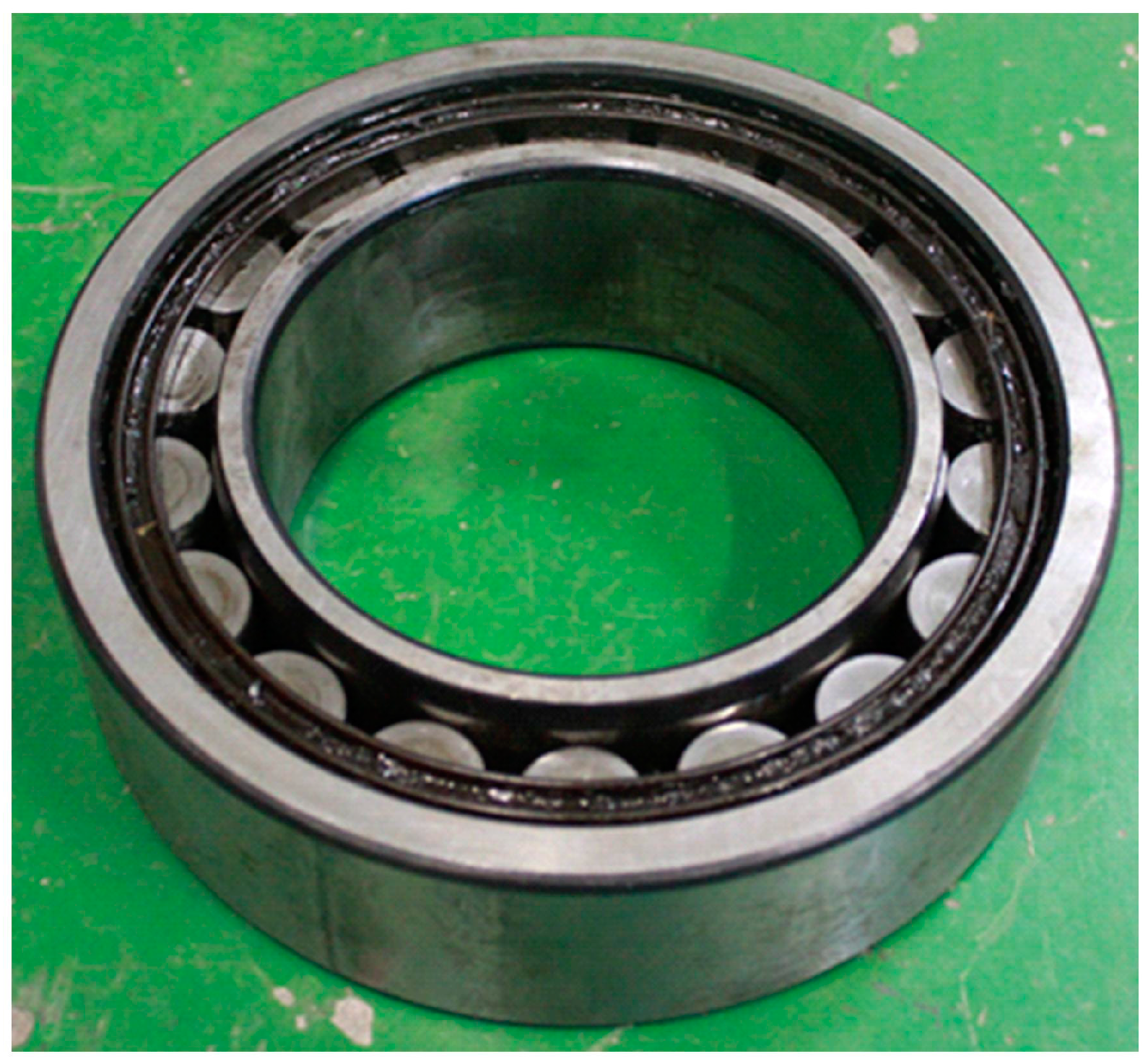
(1) The test of healthy bearing

Figure 5 shows the bearing with no fault. Figure 6a,b is the waveform of the collected vibration signals and the envelope spectrum respectively. Figure 6a shows that there is no obvious impact pulse in the time domain waveform and Figure 6b shows no peaks in the envelope spectrum at fault characteristic frequency. So, the bearing may be healthy.

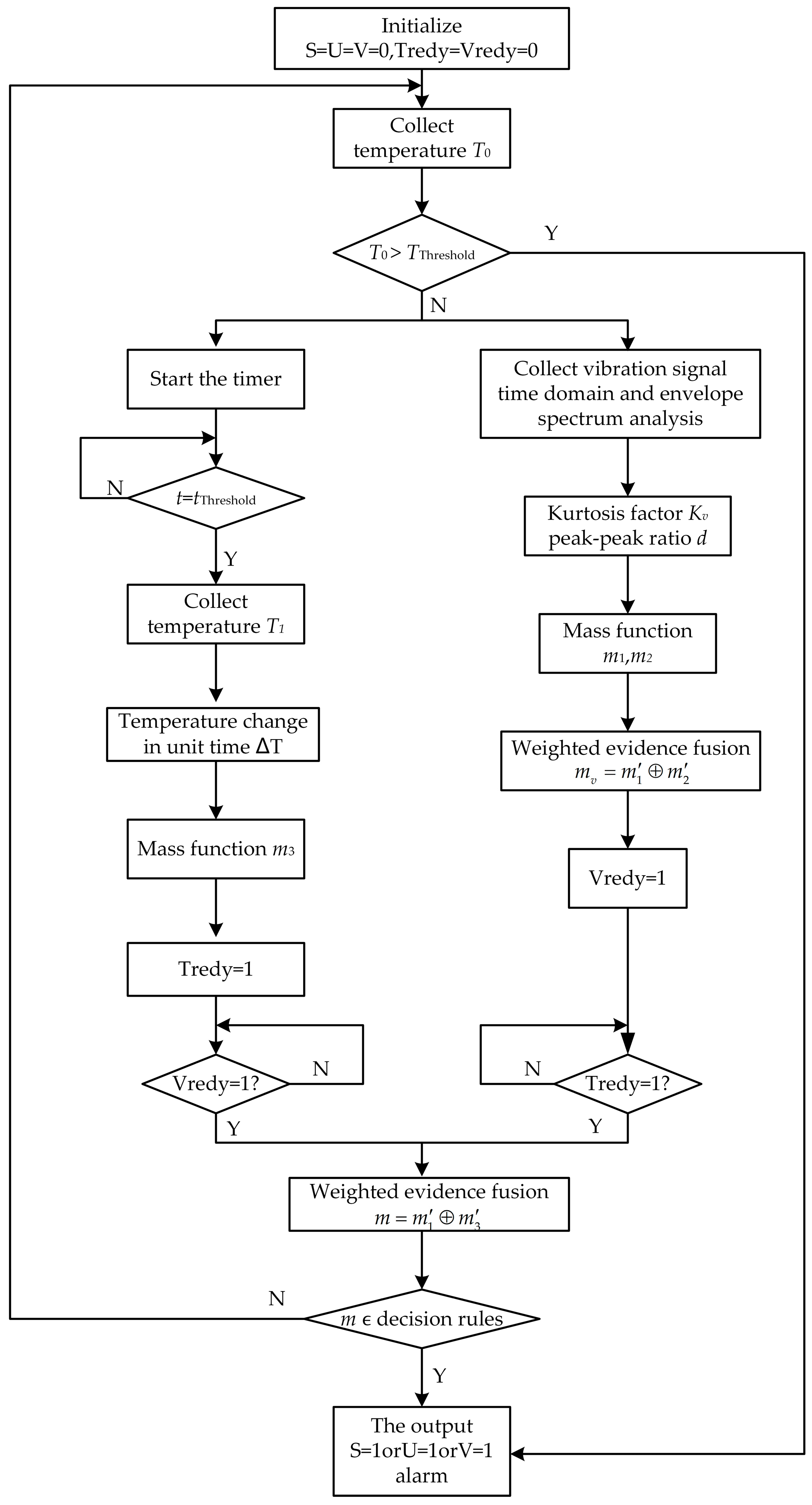
By running the designed software, which adopts WQPCDA to fuse the collected signals, the parameters extracted in the experiment are (the software contains three kinds of fault types but we show only one):

• Peak–peak ratio: P = 1.557;
• Kurtosis factor: K_v = 3.591;
• Axle box temperature: T₀ = 26.6875 °C, T₁ = 26.9375 °C, ∆T = 0.25 °C/min.

The mass functions of the three evidence sources are shown in

Table 2. The mass functions.

Mass Function	Fault	Uncertain	Normal
$m_1:(P)$	0.244	0.576	0.180
$m_2:(K_v)$	0.245	0.570	0.185
$m_3:(\Delta T)$	0.097	0.225	0.677

.

The mass functions weighted are shown in

Table 3. The weighted mass functions.

Mass Function	Fault	Uncertain	Normal
$m_1:(P)$	0.244	0.576	0.180
$m_2:(K_v)$	0.245	0.570	0.185
$m_3:(\Delta T)$	0.094	0.473	0.433

.

The fusion result based on WQPCDA is shown in

Table 4. The fusion result.

Fusion Result	Fault	Uncertain	Normal
$m$	0.017	0.860	0.123

.

From Table 4, we know that the fusion result m does not conform to the decision rules, so the diagnosis result suggests that there is no fault in the bearing, which is consistent with the actual condition.

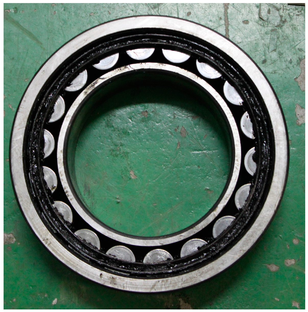
(2) The test of outer ring fault bearing

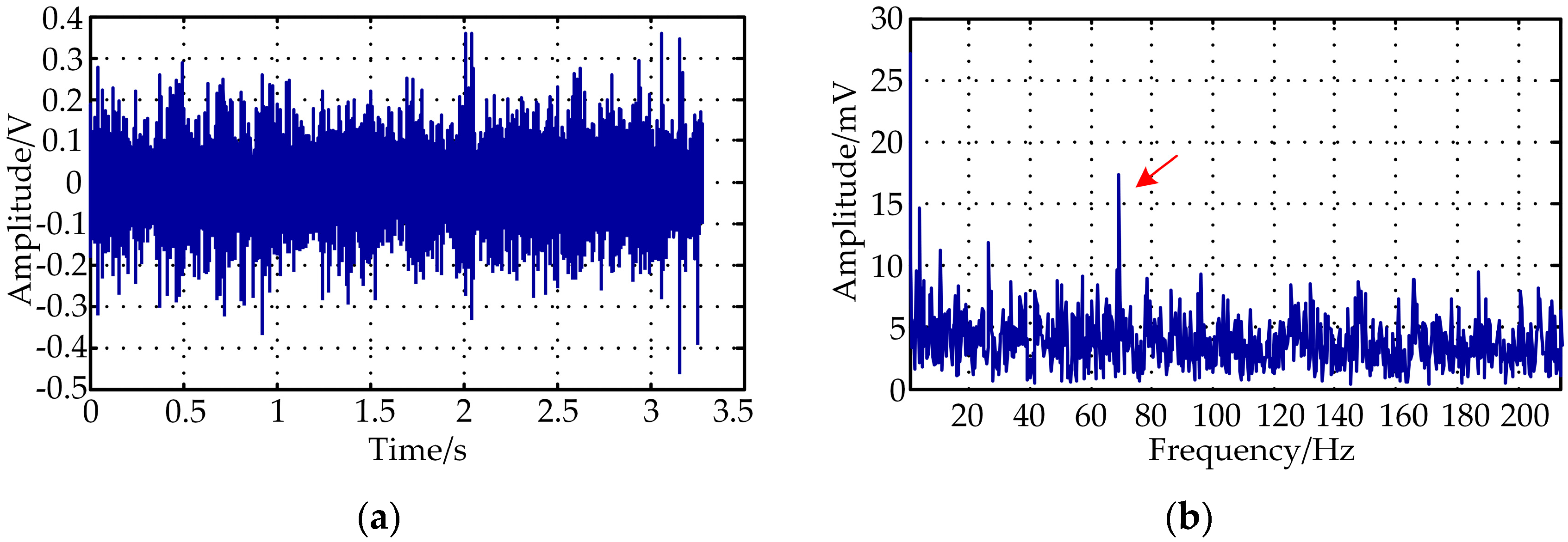
Figure 7 is the bearing with an outer ring fault. According to (28), the fault characteristic frequency of the outer ring is 69.030 Hz. Figure 8a,b shows the waveform of the collected vibration signal and the envelope spectrum respectively.

From Figure 8a, we can easily see that there is cyclical impact pulse in the time domain waveform of the original vibration signal. From Figure 8b, we can see an obvious peak in the envelope spectrum at 68.66 Hz, and this frequency belongs to the acceptable range of the outer ring fault characteristic frequency. So, there may be a fault in outer ring.

By running the designed software, the parameters extracted in the experiment are:

• Peak–peak ratio at outer ring fault characteristic frequency: P = 2.114;
• Kurtosis factor: K_v = 5.307;
• Axle box temperature: T₀ = 24.8125 °C, T₁ = 25.0 °C, ∆T = 0.1875°C/min.

The mass functions of the three evidence sources are shown in

Table 5. The mass functions.

Mass Function	Fault	Uncertain	Normal
$m_1:(P)$	0.809	0.114	0.077
$m_2:(K_v)$	0.819	0.102	0.079
$m_3:(\Delta T)$	0.102	0.233	0.665

.

The weighted mass functions are shown in

Table 6. The weighted mass functions.

Mass Function	Fault	Uncertain	Normal
$m_1:(P)$	0.809	0.114	0.077
$m_2:(K_v)$	0.819	0.102	0.079
$m_3:(\Delta T)$	0.451	0.147	0.402

.

The fusion result based on WQPCDA is shown in

Table 7. The fusion result.

Fusion Result	Fault	Uncertain	Normal
$m$	0.918	0.011	0.071

.

From Table 7, we know that the fusion result, $m$ conforms to the decision rules, so the output is S = 1.

The diagnosis result suggests that there is a fault in the outer ring, which is consistent with the actual condition. The proposed bearing fault diagnosis method is tested as being effective.

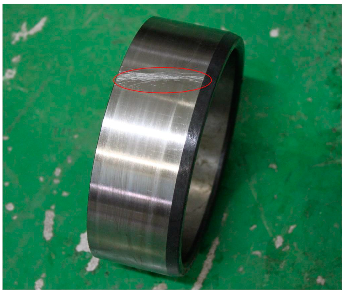
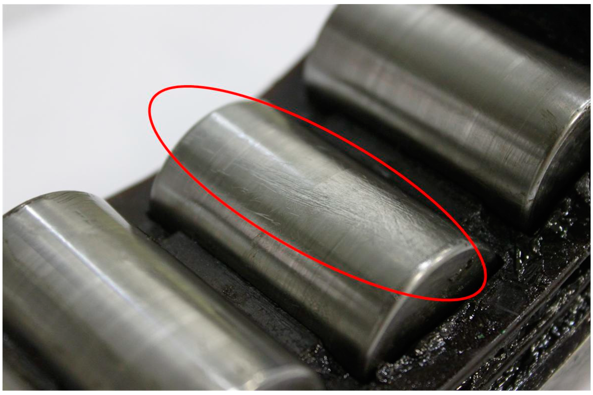
(3) The test of inner ring fault bearing

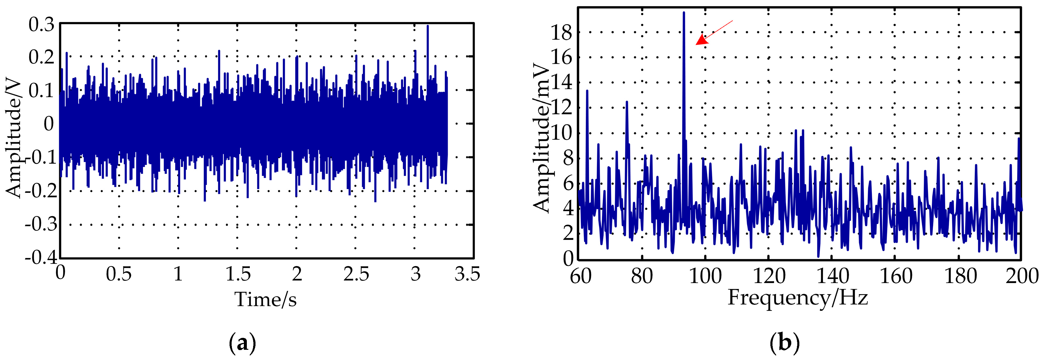
The bearing with an inner ring fault is shown in Figure 9. According to Equation (29), the fault characteristic frequency of the inner ring is 92.970 Hz. Figure 10a,b shows the waveform of the collected vibration signal and the envelope spectrum, respectively.

By running the designed software, the parameters extracted in the experiment are:

• Peak–peak ratio at inner ring fault characteristic frequency: P = 2.365;
• Kurtosis factor: K_v = 5.086;
• Axle box temperature: T₀ = 24.0 °C, T₁ = 24.0625 °C, ∆T = 0.0625 °C/min.

The mass functions of the three evidence sources are shown in

Table 8. The mass functions.

Mass Function	Fault	Uncertain	Normal
$m_1:(P)$	0.855	0.083	0.062
$m_2:(K_v)$	0.804	0.112	0.084
$m_3:(\Delta T)$	0.111	0.247	0.642

.

The weighted mass functions are shown in

Table 9. The weighted mass functions.

Mass Function	Fault	Uncertain	Normal
$m_1:(P)$	0.855	0.083	0.062
$m_2:(K_v)$	0.804	0.112	0.084
$m_3:(\Delta T)$	0.458	0.154	0.388

.

The fusion result based on WQPCDA is shown in

Table 10. The fusion result.

Fusion Result	Fault	Uncertain	Normal
$m$	0.924	0.012	0.064

.

From Table 10, we know that the fusion result, $m$ conforms to the decision rules, so the output is U = 1.

The diagnosis result suggests that there is a fault in the inner ring, and this is consistent with the actual condition. The proposed bearing fault diagnosis method is tested to be effective.

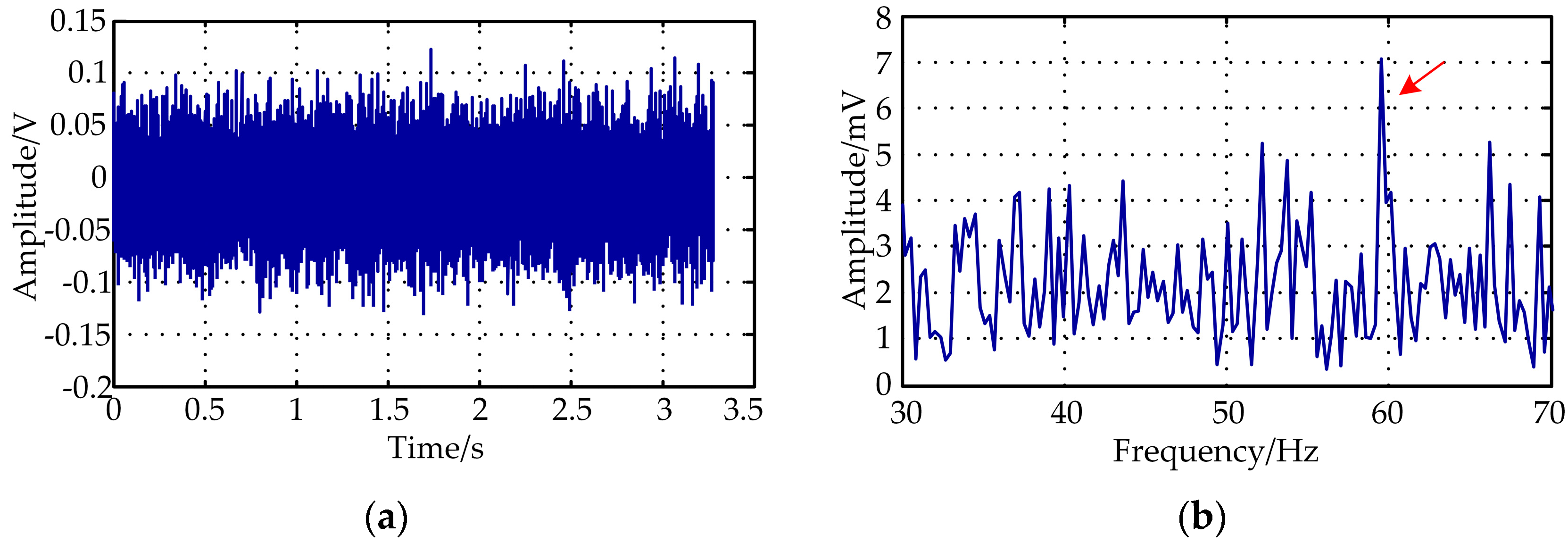
(4) The test of rolling element fault bearing

The bearing with a rolling element fault is shown in Figure 11. According to (30), the fault characteristic frequency of the rolling element is 29.796 Hz. Figure 12a,b show the waveform of the collected vibration signal and the envelope spectrum, respectively.

From Figure 12b, we can see an obvious peak in the envelope spectrum at 59.506 Hz, which belongs to the acceptable range of double frequency of rolling element faults. By running the designed software, the parameters extracted in the experiment are:

• Peak–peak ratio at rolling element fault characteristic frequency: P = 1.699;
• Kurtosis factor: K_v = 3.866;
• Axle box temperature: T₀ = 25.0625 °C, T₁ = 25.125 °C, ∆T = 0.0625 °C/min.

The mass functions of the three evidence sources are shown in

Table 11. The mass functions.

Mass Function	Fault	Uncertain	Normal
$m_1:(P)$	0.728	0.170	0.102
$m_2:(K_v)$	0.427	0.394	0.179
$m_3:(\Delta T)$	0.111	0.247	0.642

.

The mass weighted functions are shown in

Table 12. The weighted mass functions.

Mass Function	Fault	Uncertain	Normal
$m_1:(P)$	0.728	0.170	0.102
$m_2:(K_v)$	0.427	0.394	0.179
$m_3:(\Delta T)$	0.374	0.223	0.403

.

The fusion result based on WQPCDA is shown in

Table 13. The fusion result.

Fusion Result	Fault	Uncertain	Normal
$m$	0.774	0.098	0.128

.

From Table 13, we know that the fusion result, $m$ conforms to the decision rules, so the output is V = 1.

The diagnosis result suggests that there is a fault in the rolling element, and this is consistent with the actual condition. The proposed bearing fault diagnosis method is tested as being effective.

6. Experimental Study for Comparison

In order to verify that the proposed improved D-S evidence fusion algorithm is most suitable for bearing fault diagnosis, we compared it with two existing improved D-S evidence fusion algorithms (the mean K coefficient algorithm proposed by Bicheng Li, and the absorption algorithm proposed by Weitong Li) by applying them all to the bearing fault diagnosis using the same experimental data.

(1) The mean K coefficient algorithm

The main idea of this algorithm is to use the average value of mass functions to improve the result of the classic fusion algorithm when the conflict between the evidences is too large. Its formula is:

$$m(A)={\displaystyle \sum _{A_i\cap B_j=A}{m}_1(A_i)m_2(B_j)+K\cdot \frac{1}{n}{\displaystyle \sum _{i=1}^n{m}_i(A)}}$$

(35)

The algorithm is simple in that the rationality of the final result can be improved by weakening the proportion of the classical results and increasing the average proportion when the conflict increases.

(2) The absorption algorithm

The main idea of the absorption algorithm is to adaptively distribute the conflict based on the mass functions, and the weight coefficients are related to the value of mass functions. Its formula is:

$$\begin{array}{l}m(A)={\displaystyle \sum _{A_i\cap A_j=A}{m}_1(A_i)m_2(A_j)}+\{\begin{array}{c}{\displaystyle \sum _{A\cap A_j=\varphi }{m}_1(A)m_2(A_j)}\frac{m_1(A)}{m_1(A)+m_2(A_j)},m_1(A)>m_2(A)\\ {\displaystyle \sum _{A_i\cap A=\varphi }{m}_1(A_i)m_2(A)}\frac{m_2(A)}{m_1(A_i)+m_2(A)},m_2(A)>m_1(A)\end{array}\\ \end{array}$$

(36)

We collected 100 groups of data, including 20 groups of data obtained from the outer ring fault bearing under the condition of the inner ring rotating at 9 Hz and 7.5 Hz, respectively, 20 groups of data obtained from the inner ring fault bearing where the inner ring operates at 9 Hz and 7.5 Hz, respectively, and 20 groups of data obtained from the rolling element fault bearing where the inner ring operates at 9 Hz. The evidence for the peak–peak ratio, kurtosis factor and temperature variation were extracted and the mass functions were generated based on the method proposed in this paper. Finally, the proposed WQPCDA fusion algorithm, the mean K coefficient algorithm and the absorption algorithm were used to compare their accuracy. The decision threshold is set to be 0.3 as mentioned before.

We recorded the data sets which could correctly diagnose the fault. Figure 13 shows the decision values, which is defined as the smaller one of “m(Fault) − m(Uncertain)” and “m(Fault) − m(Normal)”.

In Figure 13, we can see that of 100 groups of data, our proposed algorithm and the absorption algorithm found fault in 91 groups of data so the accuracy rate is 91%. The mean K coefficient algorithm only detected 85 groups of data, so the accuracy rate is 85%. This shows that our proposed fusion algorithm and the absorption algorithm are much more suitable for evidence fusion in the field of bearing fault diagnosis compared with the mean K coefficient algorithm.

Considering the results above, we cannot determine which method is better; our proposed fusion algorithm or the absorption algorithm. Therefore, the misdiagnosis rate of these two kinds of algorithms for normal bogie bearings is considered Twenty-five groups of data for the normal bearing at 9 Hz and 7.5 Hz were collected. Our proposed fusion algorithm and the absorption algorithm were used to diagnose the fault. The results of the diagnosis of the two algorithms is shown in Figure 14.

We can see from Figure 14 that among 50 groups of no-fault data, our proposed fusion algorithm misdiagnoses once, so the misdiagnosis rate is 2%. The absorption algorithm found faults in 5 groups of data so the misdiagnosis rate is 10%. Therefore, the misdiagnosis rate of our proposed fusion algorithm is significantly smaller than that of the absorption algorithm.

In summary, the diagnosis accuracy rate of the proposed fusion algorithm and the absorption algorithm reached 91%, which is significantly better than that of the mean K coefficient algorithm. In addition, the misdiagnosis rate of the proposed fusion algorithm is only 2%, less than the 10% misdiagnosis rate of the absorption algorithm. Therefore, our proposed fusion algorithm is much more suitable for the fusion of evidence in the field of bearing fault diagnosis.

7. Conclusions

The health of bogie bearings is extremely important for the safe operation of metro vehicles. There are some deficiencies in the prevailing fault diagnosis methods for metro vehicle bogie bearings, including information simplification, poor accuracy and low diagnosis rate. This paper proposes a multi-information intelligent fault diagnosis method for metro vehicle bogie bearings, which adopts a weighted improved D-S evidence theory to detect bearing faults by analyzing vibration signals and temperature signals. Unlike classic D-S evidence theory, the proposed method modifies the fusion rules, making it much more reasonable as well as effective. To verify the effectiveness and accuracy rate of the proposed intelligent diagnosis method, bearings with outer ring, inner ring or rolling element faults were tested in a constructed bearing fault test platform. The diagnosis accuracy rate of the proposed fusion algorithm reached 91%, and the misdiagnosis rate is only 2%. The test results show that the proposed method can accurately and reliably realize fault diagnosis with a high accuracy rate and low misdiagnosis rate compared to previously used methods. In other words, this paper puts forward an effective online intelligent fault diagnosis method for bogie bearings of metro vehicles. Besides, the algorithm is simple, feasible and real-time online diagnosis is easy to realize, thus, it can be extended to all bearing fault diagnosis.

References

1. Frosini, L.; Harlisca, C.; Szabó, L. Induction machine bearing faults detection by means of statistical processing of the stray flux measurement. IEEE Trans. Ind. Electron. 2015, 62, 1846–1854. [Google Scholar] [CrossRef]
2. Henao, H.; Capolino, G.A.; Fernandez-Cabanas, M.; Filippetti, F. Trends in fault diagnosis for electrical machines: A review of diagnostic techniques. IEEE Ind. Electron. Mag. 2014, 8, 31–42. [Google Scholar] [CrossRef]
3. Hu, Q.; He, Z.; Zhang, Z.; Zi, Y. Fault diagnosis of rotating machinery based on improved wavelet package transform and SVMs ensemble. Mech. Syst. Signal Process. 2007, 21, 688–705. [Google Scholar] [CrossRef]
4. Wu, C.X.; Ning, L.W.; Jiang, R.; Wu, X.; Liu, J. Intelligent Identification of Bearing Faults Using Time Domain Features. In Proceedings of the 2013 Fourth International Conference on Digital Manufacturing & Automation, Qingdao, China, 29–30 June 2013; pp. 713–716. [Google Scholar]
5. Borghesani, P.; Pennacchi, P.; Randall, R.B.; Sawalhi, N.; Ricci, R. Application of cepstrum pre-whitening for the diagnosis of bearing faults under variable speed conditions. Mech. Syst. Signal Process. 2013, 36, 370–384. [Google Scholar] [CrossRef]
6. Kankar, P.K.; Sharma, S.C.; Harsha, S.P. Fault diagnosis of rolling element bearing using cyclic autocorrelation and wavelet transform. Neurocomputing 2013, 110, 9–17. [Google Scholar] [CrossRef]
7. Bin, G.F.; Gao, J.J.; Li, X.J.; Dhillon, B.S. Early fault diagnosis of rotating machinery based on wavelet packets—Empirical mode decomposition feature extraction and neural network. Mech. Syst. Signal Process. 2012, 27, 696–711. [Google Scholar] [CrossRef]
8. Zadeh, L.A. Fuzzy Sets. Inf. Control 1965, 338–353. [Google Scholar] [CrossRef]
9. Xia, X.T.; Chen, L. Fuzzy chaos method for evaluation of nonlinearly evolutionary process of rolling bearing performance. Measurement 2013, 46, 1349–1354. [Google Scholar] [CrossRef]
10. de Moura, E.P.; Souto, C.R.; Silva, A.A.; Irmão, M.A.S. Evaluation of principal component analysis and neural network performance for bearing fault diagnosis from vibration signal processed by RS and DF analyses. Mech. Syst. Signal Process. 2011, 25, 1765–1772. [Google Scholar] [CrossRef]
11. Barakat, M.; El Badaoui, M.; Guillet, F. Hard competitive growing neural network for the diagnosis of small bearing faults. Mech. Syst. Signal Process. 2013, 37, 276–292. [Google Scholar] [CrossRef]
12. Guan, K.; Mei, T.; Wang, D.J. Application of multi-sensor information fusion in fault diagnosis of rotating machinery. In Proceedings of the IEEE ICIA 2006—2006 IEEE International Conference on Information Acquisition, Weihai, China, 20–23 August 2006; pp. 425–429. [Google Scholar]
13. Yager, R.R. On the dempster-shafer framework and new combination rules. Inf. Sci. 1987, 41, 93–137. [Google Scholar] [CrossRef]
14. Murphy, C.K. Combining belief functions when evidence conflicts. Decis. Support Syst. 2000, 29, 1–9. [Google Scholar] [CrossRef]
15. Hang, J.; Zhang, J.Z.; Chen, M. Fault diagnosis of wind turbine based on multi-sensors information fusion technology. IET Renew. Power Gener. 2014, 8, 289–298. [Google Scholar] [CrossRef]
16. Shi, H.B.; Yang, S.Y.; Cao, Z.L.; Pan, W.; Li, W. An improved evidence combination method of D-S theory. In Proceedings of the 2016 International Symposium on Computer, Consumer and Control, Xi’an, China, 4–6 July 2016; pp. 319–322. [Google Scholar]
17. Zhou, J.; Liu, H.; Chen, Y.; Li, Z. Research on the fault characteristics and fault diagnosis methods of three-level high-power inverter. In Proceedings of the 2009 IEEE 6th International Power Electronics and Motion Control Conference, Wuhan, China, 17–20 May 2009; Volume 43, pp. 892–896. [Google Scholar]
18. Le Hégarat-Mascle, S.; Bloch, I.; Vidal-Madjar, D. Application of Dempster—Shafer Evidence Theory to Unsupervised Classification in Multisource Remote Sensing. IEEE Trans. Geosci. Remote Sens. 1997, 35, 1018–1031. [Google Scholar] [CrossRef]
19. Lu, L.; Xie, W.; Zhang, J.; Huang, G.; Li, Q.; Zhao, Z. Woodland extraction from high-resolution CASMSAR data based on dempster-shafer evidence theory fusion. Remote Sens. 2015, 7, 4068–4091. [Google Scholar] [CrossRef]
20. Li, W.; Bao, J.; Fu, X.; Fortino, G.; Galzarano, S. Human postures recognition based on D-S evidence theory and multi-sensor data fusion. In Proceedings of the 12th IEEE/ACM International Symposium on Cluster, Cloud and Grid Computing, Ottawa, ON, Canada, 13–16 May 2012; Volume 59, pp. 912–917. [Google Scholar]
21. Wang, H.; Lin, D.; Qiu, J.; Ao, L.; Du, Z.; He, B. Research on multiobjective group decision-making in condition-based maintenance for transmission and transformation equipment based on D-S evidence theory. IEEE Trans. Smart Grid 2015, 6, 1035–1045. [Google Scholar] [CrossRef]
22. Lin, T.C.; Yu, P.T. Thresholding noise-free ordered mean filter based on Dempster-Shafer theory for image restoration. IEEE Trans. Circuits Syst. I Regul. Pap. 2006, 53, 1057–1064. [Google Scholar]
23. Tao, B.; Zhu, L.; Ding, H.; Xiong, Y. An alternative time-domain index for condition monitoring of rolling element bearings-A comparison study. Reliab. Eng. Syst. Saf. 2007, 92, 660–670. [Google Scholar] [CrossRef]
24. Liu, J.Q.; Zhao, Z.B.; Zhang, G.P.; Wang, G.M.; Meng, S.; Ren, G. Research on the Fault Diagnosis Method for Bogie Bearings of the Metro Vehicle. J. China Railw. Soc. 2015, 37, 30–36. (In Chinese) [Google Scholar]
Figure 1. Three-layer wavelet packet decomposition tree.
Energies 11 00232 g001
Figure 2. The flow table of bearing fault diagnosis.
Energies 11 00232 g002
Figure 3. Schematic diagram of the test platform.
Energies 11 00232 g003
Figure 4. The physical test platform.
Energies 11 00232 g004
Figure 5. The healthy bearing.
Energies 11 00232 g005
Figure 6. The waveform of the healthy bearing vibration signal. (a) Time domain waveform; (b) envelope spectrum waveform.
Energies 11 00232 g006
Figure 7. The outer ring fault bearing.
Energies 11 00232 g007
Figure 8. The waveform of outer ring fault bearing vibration signal. (a) Time domain waveform; (b) envelope spectrum waveform.
Energies 11 00232 g008
Figure 9. The inner ring fault bearing.
Energies 11 00232 g009
Figure 10. The waveform of the inner ring fault bearing vibration signal. (a) Time domain waveform; (b) envelope spectrum waveform.
Energies 11 00232 g010
Figure 11. The rolling element fault bearing.
Energies 11 00232 g011
Figure 12. The waveform of the rolling element fault bearing vibration signal. (a) Time domain waveform; (b) envelope spectrum waveform.
Energies 11 00232 g012
Figure 13. Comparison of the accuracy rate of the 3 improved algorithms. (a) data for the inner ring fault at 9 Hz; (b) data for the inner ring fault at 7.5 Hz; (c) data for the outer ring fault at 9 Hz; (d) data for the outer ring fault at 7.5 Hz; (e) data for the rolling element fault at 9 Hz.
Energies 11 00232 g013
Figure 14. Comparison of the misdiagnosis rate of our proposed fusion algorithm and the absorption algorithm.
Energies 11 00232 g014